Return to Article Details About B-splines. Twenty answers to one question: What is the cubic B-spline for the knots -2,-1,0,1,2?

About B-splines. Twenty answers to one question: What is the cubic B-spline for the knots -2,-1,0,1,2?

Ewald Quak $^{*}$

February 9, 2016.

$^{*}$ October 22, 2004. SINTEF Applied Mathematics, Oslo, Norway.
This article by the late Ewald Quak is published with the consent of his wife Riina and upon the initiative of a member of the editorial board of this journal. It is followed by some comments of Carl de Boor on early Bulgarian and Romanian contributions to B-splines.

In this composition an attempt is made to answer one simple question only: What is the cubic B-spline for the knots -2,-1,0,1,2? The note will take you on a most interesting trip through various fields of Mathematics and finally convince you on how little we know.

MSC. 41-XX, 65-XX, 60-XX

Keywords. cubic B-spline, curves and surfaces, CAD-CAM, Approximation Theory, Numerical Analysis, Probability.

1 Introduction

Polynomial splines are real-valued functions which consist of polynomial pieces that are glued together at given breakpoints with prescribed smoothness. To name just a few applications of these powerful tools within applied and computational mathematics: splines are a de-facto standard in the mathematical description of curves and surfaces for industrial computer-aided design and manufacture (CAD-CAM). Spline surfaces and their offspring subdivision surfaces are at the heart of professional animation systems for the production of movies like Toy Story or Monsters, Inc. Splines are also used to solve ordinary differential equations and in the multivariate form of finite elements they form the cornerstone for the numerical treatment of partial differential equations. The approximation of scattered data, be it in geometric modelling or statistics, can be carried out with splines. Wavelet theory and multiresolution analysis owe a lot to spline functions as well.

\includegraphics[scale=0.5]{bspline.png} — Figure 1 The graph of the cubic B-spline for the knots -2,-1,0,1,2.

So both faculty and students are bound to encounter splines in very different settings and basic spline material is to some extent incorporated in undergraduate numerical analysis text books. In this paper I would like to give some examples how a certain B-spline basis function can be characterized. Some of these examples are well-known and at the heart of important theory or applications, other disguises are rather far-fetched, and could be considered as dragged from mathematical oblivion. I do not claim that this list is in any way complete, and I invite all readers to supply me with other approaches they have encountered.

In this text, I have deliberately chosen to focus on cubic splines and consequently not formulated any statements in the highest possible generality. In this way I hope to generate more questions rather than give complete answers, stimulating the reader’s interest to take a closer look –for example at other spline degrees or different choices of breakpoints. Some remarks in this direction are given in the final section of the paper. I tried to hold the proofs as elementary as possible, but still giving a flavor of what is happening in more general situations, avoiding - if possible - straightforward calculations just valid for the cubic case. As for the sources that inspired my twenty answers, I tried to quote early original papers, but are not in a position to claim absolute historical accuracy concerning who did what first. Instead the reader is invited to consult on his or her own more detailed spline monographs, or study books dealing with a specific application area using splines. Be aware, however, that it was of course necessary to change original notations and also proofs to generate a consistent presentation.

The twenty choices are listed in Section 2, including the references that inspired them. The first answer is discussed in Section 3 and allows to say a bit where the name spline originated. Using yet another definition we are able to address in Section 4 some basic properties in items 2, 3 and 4, including the basis property that motivated the term B-spline as in basis spline. In the subsequent Section 5, divided differences of truncated power functions allow us to come up with a closed formula expression, point out connections to Green’s functions and Peano kernels, and give a geometric interpretation in items 5-8. Fourier transforms are employed in Section 6 for items 9-11. Subdivision concepts, important in wavelet theory and geometric modeling, are then showcased in Section 7 for items 12 and 13. Section 8 is devoted to probability interpretations in items 14-17, including the historic reference from 1904, where the graph of a cubic B-spline (probably) appears for the first time, years before the term B-spline was coined. Also the last items 18-20 covered in Section 9 stem from roots in probability, but are singled out because they originated in the author’s country of residence. The final Section 10 tries to give some information how the general spline theory can be developed from the cubic approach in this elementary paper and where to find the relevant information. Enjoy!

2 Twenty choices

[ 44 , 27 ] The function $f$ which minimizes the integral

$\int_{- 2}^{2} {(g^{''} (x))}^{2} d x,$

when considering all functions $g$ , whose second derivatives are square integrable over the interval $[- 2; 2]$ and which interpolate the following data:

$g (- 2) = g^{'} (- 2) = g (2) = g^{'} (2) = 0, g (- 1) = g (1) = \frac{1}{6}, g (0) = \frac{2}{3} ?$
[ 38 ] The function $f$ defined by the pieces

$f (x) = {\begin{cases} \frac{1}{6} {(x + 2)}^{3}, & if x \in [- 2, - 1], \\ \frac{1}{6} ({(x + 2)}^{3} - 4 {(x + 1)}^{3}), & if x \in [- 1, 0], \\ \frac{1}{6} ({(2 - x)}^{3} - 4 {(1 - x)}^{3}), & if x \in [0, 1], \\ \frac{1}{6} {(2 - x)}^{3}, & if x \in [1, 2], \\ 0, & otherwise. \end{cases} ?$
[ 13 ] The function $f$ of smallest support such that $f$ is a cubic polynomial on each interval $[k; k + 1]$ for each $k \in Z$ , twice continuously differentiable everywhere, even and for which $f (0) = \frac{2}{3} ?$
[ 2 , 12 ] The function $f$ built from characteristic functions as

$\begin{aligned} f (x) & = \frac{x + 2}{3} (\frac{x + 2}{2} ((x + 2) X_{| [- 2, - 1)} (x) + (- x) X_{| [- 1, 0)} (x)) \\ + \frac{1 - x}{2} ((x + 1) X_{| [- 1, 0)} (x) + (1 - x) X_{| [0, 1)} (x))) \\ + \frac{2 - x}{2} (\frac{x + 1}{2} ((x + 1) X_{| [0, 1)} (x) + (1 - x) X_{| [0, 1)} (x)) \\ + \frac{2 - x}{2} ((x) X_{| [0, 1)} (x) + (2 - x) X_{| [1, 2)} (x))) . \end{aligned}$

where for $k = - 2, - 1, 0, 1$

$X_{| [k, k + 1)} = {\begin{cases} 1 & if\ x \in [k, k + 1), \\ 0 & if\ x \notin [k, k + 1) \end{cases} ?$
[ 38 ] The function $f$ given by

$f (x) = \frac{1}{6} ({(- 2 - x)}_{+}^{3} - 4 {(- 1 - x)}_{+}^{3} + 6 {(- x)}_{+}^{3} - 4 {(1 - x)}_{+}^{3} + {(2 - x)}_{+}^{3}),$

where the truncated power functions are defined as $x_{+} = max (x, 0)$ and $x_{+}^{3} = {(x_{+})}^{3} ?$
[ 5 ] The function $f$ obtained by taking the divided difference with respect to t in the points $- 2, - 1, 0, 1, 2$ of Green’s function associated with the differential operator $D^{4}$ and multiplying the result by 24? This means

$f (x) = 24 {[- 2, - 1, 0, 1, 2]}_{t} G_{4} (t, x),$

where for any given function $h$ which is integrable on $[- 2, 2]$ and any real numbers $g_{0}, g_{1}, g_{2},$ $g_{3}$ the function

$g (t) = \sum_{j = 0}^{3} g_{j} \frac{{(t + 2)}^{j}}{j!} + \int_{- 2}^{2} G_{4} (t, x) h (x) d x$

solves the initial value problem

$\begin{aligned} g^{(4)} (t) & = h (t), \ \ \ \ \ almost everywhere in [- 2, 2], \\ g^{(ℓ)} (- 2) & = g_{ℓ}, ℓ = 0, 1, 2, 3. \end{aligned}$
[ 13 ] The function $f$ for which

$\int_{- \infty}^{+ \infty} f (x) h^{(4)} (x) d x = △^{4} h (0),$

for all functions $h$ , which are four times continuously differentiable on $[- 2, 2]$ , and where $△^{4} h (x)$ is the fourth order central difference defined as

$△^{4} h (x) = △ (△ (△ (△ h (x)))), \ with △ h (x) = h (x + \frac{1}{2}) - h (x - \frac{1}{2}) ?$
[ 13 ] The function $f$ so that $f (x)$ represents the 3-dimensional volume of the intersection of a hyperplane in $R^{4}$ that is orthogonal to the $x$ -axis and goes through the point $(x, 0, 0, 0)$ with a 4-simplex of volume 1, which is placed in $R^{4}$ , so that its five vertices project orthogonally onto the points on the $x$ -axis $(- 2, 0, 0, 0), (- 1, 0, 0, 0), (0, 0, 0, 0), (1, 0, 0, 0),$ $(2, 0, 0, 0)$ ?
[ 38 ] The function $f$ whose Fourier transform is the $4 t h$ power of a dilated sinc function, i.e., using the inverse Fourier transform

$f (x) = \frac{1}{2 π} \int_{- \infty}^{+ \infty} {(\frac{\sin (\frac{u}{2})}{\frac{u}{2}})}^{4} e^{i x u} d u ?$
[ 38 ] The function $f$ which results when taking the convolution of the hat function

$N (x) = {\begin{cases} x + 1, & if\ x \in [- 1, 0], \\ 1 - x, & if\ x \in [0, 1], \\ 0, & otherwise, \end{cases}$

with itself, i.e.,

$f (x) = (N * N) (x) = \int_{- \infty}^{+ \infty} N (x - y) N (y) d y, x \in R ?$
[ 36 , 28 ] The function $f$ generated in the following way?

In $R^{2}$ a unit square is placed with its lower edge on the $x$ -axis and then moved along this axis. Assuming the square’s center at time $x$ to be the point $(x, \frac{1}{2})$ , we obtain a function $A$ such that $A (x)$ is the area of the region cut out of the square by the graph of the hat function $N (x)$ (see item 10) and the $x$ -axis. Repeating this process one more time, we obtain $f (x)$ as the area of the region cut out of the square by the graph of the function $A (x)$ and the $x$ -axis.
[ 8 ] The continuous function $f$ which has the values $f (0) = \frac{2}{3},$ $f (1) = f (- 1) = \frac{1}{6},$ and $0$ in all other integers and satisfies the functional equation

$f (x) = \frac{1}{8} (f (2 x + 2) + 4 f (2 x + 1) + 6 f (2 x) + 4 f (2 x - 1) + f (2 x - 2)) ?$
[ 34 , 9 ] The continuous function $f$ which results from the following limit process?

We start with the polygon in $R^{2}$ that connects the initial points $P_{k}^{0} = (k, δ_{k, 0})$ . Then we generate new polygons successively by setting for $r \in N \cup {0}$ and any $k \in Z$

$\begin{aligned} P_{2 k}^{r + 1} & = \frac{1}{8} (P_{k - 1}^{r} + 6 P_{k}^{r} + P_{k + 1}^{r}), \\ P_{2 k + 1}^{r + 1} & = \frac{1}{2} (P_{k}^{r} + P_{k + 1}^{r}) . \end{aligned}$

The resulting polygons converge to $f$ in the sense that for $r \in N \cup {0}$ and any $k \in Z$

${‖ (\frac{k}{2^{r}}, f (\frac{k}{2^{r}})) - P_{k}^{r} ‖}_{\infty} \leq \frac{1}{3} \frac{1}{2^{r}} .$
[ 25 ] The function $f$ describing the discrete probability distribution for the following urn model?

Consider an urn initially containing w white balls and b black balls. One ball at a time is drawn at random from the urn and its color is inspected. Then it is returned to the urn and $w + b$ balls of the opposite color are added to the urn. A total of three such draws are carried out. With $t = w / (w + b)$ as the probability of selecting a white ball on the first trial, the probability of selecting exactly 3 white balls in the three trials is $f (t - 2)$ , of selecting exactly 2 white balls in the three trials is $f$ $(t - 1)$ , of selecting exactly 1 white ball in the three trials is $f (t)$ and of selecting exactly $0$ white balls in the three trials is $f (t + 1)$ .
[ 38 , 43 ] The function $f$ that is the density distribution of the error committed in the sum $X_{1} + X_{2} + X_{3} + X_{4}$ of 4 independent real random variables $X_{k}$ , if each variable is replaced by its nearest integer value?
[ 43 ] The function $f$ , such that $f (x)$ is the 3-dimensional volume of the section of the 4-dimensional unit cube ${[- \frac{1}{2}, \frac{1}{2}]}^{4}$ cut out by the hyperplane $x_{1} + x_{2} + x_{3} + x_{4} = x$ , which lies normal to the cube’s main diagonal (connecting $(- \frac{1}{2}, - \frac{1}{2}, - \frac{1}{2}, - \frac{1}{2})$ to $(\frac{1}{2}, \frac{1}{2}, \frac{1}{2}, \frac{1}{2})$ )?
[ 43 ] The function $f$ whose graph appears in the contribution of A. Sommerfeld to the Festschrift Ludwig Boltzmann gewidmet zum 60. Geburtstage, the monograph dedicated to the 60th birthday of Ludwig Boltzmann, February 20th 1904?
[ 6 ] The function $f$ so that

$f (x) = \frac{1}{π} \int_{x - \frac{1}{2}}^{x + \frac{1}{2}} \int_{t_{3} - \frac{1}{2}}^{t_{3} + \frac{1}{2}} \int_{t_{2} - \frac{1}{2}}^{t_{2} + \frac{1}{2}} (Q (t_{1} + \frac{1}{2}) - Q (t_{1} - \frac{1}{2})) d t_{1} d t_{2} d t_{3},$

where

$Q (t) = lim_{λ \to 0^{+}} \arctan (\frac{t}{λ}) ?$
[ 23 ] The function $f$ given by the real part of a complex integral in the following way:

$f (x) = \frac{8}{π} Re \int_{0}^{+ \infty} \frac{u^{3}}{(4^{2} + {(u - 2 i x)}^{2}) (2^{2} + {(u - 2 i x)}^{2}) (u - 2 i x)} d u ?$
[ 23 ] The function $f$ represented as

$f (x) = \frac{1}{12} \sum_{k = 0}^{4} {(- 1)}^{k} (\binom{4}{k}) {| x + 2 - k |}^{3} s i g n {(x + 2 - k)}^{4} ?$

3 Prelude: why is a spline called a spline?

One of the most important and straightforward things one wishes to do in numerical analysis is to interpolate given values using some simple basic functions, for example algebraic or trigonometric polynomials. Concerning interpolation by algebraic polynomials, however, it has been known for over a hundred years [ 35 ] that an interpolant can display enormous oscillations, even if the data is taken from a smooth well-behaved function. One of the ideas used to counter this effect is to consider functions that consist of various simple pieces which are glued together with a given smoothness.

3.1 The complete cubic spline interpolant

Here we will try cubic polynomial pieces connected in such a way that they form a function that is twice continuously differentiable everywhere. The places where different pieces meet are typically called breakpoints or knots. In this sense let us consider the following example.

(Interpolation) Given the five abscissae $t_{0} < t_{1} < t_{2} < t_{3} < t_{4},$ we wish to find an interpolating cubic spline function $s$ , meaning that

\begin{aligned} s & \in C^{2} [t_{0}, t_{4}], \\ s_{| [t_{k}, t_{k + 1}]} & \in Π_{3} \   \  for\   \ k = 0, 1, 2, 3, \\ s (t_{k}) & = g_{k} \   \   \  for\   \ k = 0, 1, 2, 3, 4 \end{aligned}

for prescribed real values $g_{k}$ .

Is this problem even well-posed in the sense that there exists a unique solution amongst all the piecewise cubic $C^{2}$ functions on $[t_{0}, t_{4}]$ with interior breakpoints in $t_{1} < t_{2}$ $< t_{3}$ ? The function $s$ must be a cubic polynomial $p$ on the interval $[t_{0}, t_{1}]$ , giving us 4 parameters. Since we have $C^{2}$ continuity in the point $t_{1}$ , we must have $s (x) = p (x) + a_{1} (x - t_{1})^{3}$ on the interval $[t_{1}, t_{2}]$ , and analogously $s (x) = p (x) + a_{1} (x - t_{1})^{3} + a_{2} (x - t_{2})^{3}$ on $[t_{2}, t_{3}]$ and $s (x) = p (x) + a_{1} (x - t_{1})^{3} + a_{2} (x - t_{2})^{3} + a_{3} (x - t_{3})^{3}$ on $[t_{3}, t_{4}]$ . This means we have in total seven parameters and five interpolation conditions to satisfy, so if – as we just expect, but do not know precisely right now – the conditions are independent, we still have two parameters to fix by other conditions. There are many choices for the additional two conditions, typically involving the two endpoints of the interval. One such choice is $s^{''} (t_{0}) = s^{''} (t_{4}) = 0$ [ 27 ] , but that actually influences the approximation quality in the endpoints negatively ( [ 3 ] , p. 55). Another prominent choice, which we consider here, is to prescribe Hermite data in the endpoints [ 44 ] , i.e., demanding in addition

s^{'} (t_{0}) = g_{0}^{'} \   \  and \ s^{'} (t_{4}) = g_{4}^{'},

3.2

yielding what is called a complete cubic spline interpolant $s$ .

To show properly the existence and uniqueness of the complete spline interpolant, we can proceed as in the early days of splines and set directly

s_{| [t_{k}, t_{k + 1}]} (x) = A_{k} + B_{k} (x - t_{k}) + C_{k} {(x - t_{k})}^{2} + D_{k} {(x - t_{k})}^{3}, k = 0, 1, 2, 3.

We get from the interpolation conditions (3.1) and the continuity in the break-points, with $h_{k} = t_{k + 1} - t_{k},$ for $k = 0, 1, 2, 3$

\begin{aligned} A_{k} & = g_{k} \\ h_{k} B_{k} + h_{k}^{2} C_{k} + h_{k}^{3} D_{k} & = g_{k + 1} - g_{k} . \end{aligned}

The continuity of the first derivatives then yields

B_{k} + 2 h_{k} C_{k} + 3 h_{k}^{2} D_{k} = B_{k + 1} \  for k = 0, 1, 2,

3.5

and the continuity of the second derivative

2 C_{k} + 6 h_{k} D_{k} = 2 C_{k + 1} \  for k = 0, 1, 2.

3.6

Using as principal unknowns the $C_{k} = \frac{1}{2} s^{''} (t_{k})$ for $k = 0, 1, 2, 3$ as well as $C_{4}$ as an additional variable, we get for $k = 0, 1, 2$ from (3.6) $k = 3$

D_{k} = \frac{C_{k + 1} - C_{k}}{3 h_{k}}, \quad for k = 0, 1, 2, 3.

3.7

Then (3.4) yields

B_{k} = \frac{g_{k + 1} - g_{k}}{h_{k}} - \frac{1}{3} h_{k} (2 C_{k} + C_{k + 1}), \quad for k = 0, 1, 2, 3.

3.8

Finally, the equations (3.8) and (3.7) substituted into (3.5) yield the linear system

(\begin{array}{ccccc} h_{0} & 2 (h_{0} + h_{1}) & h_{1} & 0 & 0 \\ 0 & h_{1} & 2 (h_{1} + h_{2}) & h_{2} & 0 \\ 0 & 0 & h_{2} & 2 (h_{2} + h_{3}) & h_{3} \end{array}) (\begin{matrix} C_{0} \\ C_{1} \\ C_{2} \\ C_{3} \\ C_{4} \end{matrix}) = 3 g_{I}

with the right hand side

g_{I} = {(\frac{g_{2} - g_{1}}{h_{1}} - \frac{g_{1} - g_{0}}{h_{0}}, \frac{g_{3} - g_{2}}{h_{2}} - \frac{g_{2} - g_{1}}{h_{1}}, \frac{g_{4} - g_{3}}{h_{3}} - \frac{g_{3} - g_{2}}{h_{2}})}^{T} .

The two additional Hermite conditions (3.2) in the endpoints mean that

B_{0} = g_{0}^{'} \  and B_{3} + 2 h_{3} C_{3} + 3 h_{3}^{2} D_{3} = g_{4}^{'},

resulting in the final tridiagonal $5 \times 5$ system

(\begin{array}{ccccc} 2 h_{0} & h_{0} 0 & 0 & 0 & 0 \\ h_{0} & 2 (h_{0} + h_{1}) & h_{1} & 0 & 0 \\ 0 & h_{1} & 2 (h_{1} + h_{2}) & h_{2} & 0 \\ 0 & 0 & h_{2} & 2 (h_{2} + h_{3}) & h_{3} \\ 0 & 0 & 0 & h_{3} & 2 h_{3} \end{array}) (\begin{matrix} C_{0} \\ C_{1} \\ C_{2} \\ C_{3} \\ C_{4} \end{matrix}) = 3 g

3.9

with

g = {(\frac{g_{1} - g_{0}}{h_{0}} - g_{0}^{'}, g_{I}, g_{4}^{'} - \frac{g_{4} - g_{3}}{h_{3}})}^{T} .

The coefficient matrix is diagonally dominant, and so there exists a unique solution of $C_{k}^{'} s$ , from which all the other parameters can be computed, yielding a unique complete cubic spline interpolant $s$ for the prescribed interpolation conditions (3.1) and (3.2). Clearly, the whole deduction can be carried out for any number $n$ of distinct interior breakpoints and Hermite endpoint conditions.

3.2 An extremal property

The complete cubic spline interpolant $s$ has a very special extremal property. If we take any other function $g$ that possesses a square-integrable second derivative on $[t_{0}, t_{4}]$ and interpolates the given function values $g_{k}$ in the abscissae $t_{k}$ , and in addition the derivative values $g_{0}^{'}$ and $g_{4}^{'}$ in the endpoints, we have the following integral relation between $s$ and $g$

\int_{t_{0}}^{t_{4}} (g^{''} (x) - s^{''} (x)) s^{''} (x) d x = 0,

3.10

because integration by parts yields

\int_{t_{0}}^{t_{4}} (g^{''} (x) - s^{''} (x)) s^{''} (x) d x = - \int_{t_{0}}^{t_{4}} (g^{'} (x) - s^{'} (x)) s^{'''} (x) d x,

as the remaining terms vanish due to the derivative interpolation (3.2) in the interval endpoints. Since $s^{'''}$ is piecewise constant, namely $6 D_{k}$ on the interval $[t_{k}, t_{k + 1}]$ , we can split the integral to obtain

\begin{aligned} \int_{t_{0}}^{t_{4}} (g^{''} (x) - s^{''} (x)) s^{''} (x) d x \\ = - \sum_{k = 0}^{3} 6 D_{k} \int_{t_{k}}^{t_{k + 1}} (g^{'} (x) - s^{'} (x)) d x \\ = - \sum_{k = 0}^{3} 6 D_{k} ((g (t_{k + 1}) - s (t_{k + 1})) - (g (t_{k}) - s (t_{k}))) = 0 \end{aligned}

due to the interpolation conditions (3.1), establishing (3.10). This relation, however, implies for any such interpolatory $g$ a Pythagorean integral equation

\int_{t_{0}}^{t_{4}} {(g^{''} (x))}^{2} d x = \int_{t_{0}}^{t_{4}} {(g^{''} (x) - s^{''} (x))}^{2} d x + \int_{t_{0}}^{t_{4}} {(s^{'} (x))}^{2} d x,

so that

\int_{t_{0}}^{t_{4}} {(s^{''} (x))}^{2} d x \leq \int_{t_{0}}^{t_{4}} {(g^{''} (x))}^{2} d x

3.11

with equality only if $g = s$ .

So $s$ is the unique function among all the interpolants for the specific interpolation conditions (3.1) and (3.2) which possesses minimal 2-norm of the second derivative. Again, this holds for all sets of distinct breakpoints in an interval $[a, b]$ .

Note that the integral relation (3.10) and thus the extremal property (3.11) also hold in the case, where the Hermite boundary interpolation conditions (3.2) are replaced by the conditions $s^{''} (t_{0}) = s^{''} (t_{4}) = 0$ [ 27 ] , and with suitable boundary conditions similar properties can be derived for other odd spline degrees [ 1 ] .

3.3 This why a spline is called a spline

Finally, we can address the title question of this section. From differential geometry we know that the curvature of a curve, which is given as the graph $(x, g (x))$ of a smooth function $g$ over an interval $[a, b]$ , can be described locally by the formula

κ (x) = \frac{g^{''} (x)}{{(1 + {(g^{'} (x))}^{2})}^{3 / 2}} .

Instead of minimizing the strain energy $\int$ $κ^{2} (x) d x$ of such a curve that is to pass through given points, one can simplify by just minimizing $\int {(g^{''} (x))}^{2} d x$ . From the previous subsection we know that the optimal function in this latter case is in fact the cubic spline interpolant. Keep in mind, though, that only if $| g^{'} |$ is really small, then the curvature $κ$ is actually close to $g^{''}$ .

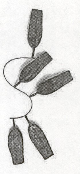
Certain instruments used in naval architecture for the construction of a smooth curve through given points were called splines, and it is for this reason the name spline was introduced in the pioneering work of I. J. Schoenberg [ 38 ] , p. 48: For $k = 4$ (polynomial order = degree $+ 1$ ) they (the curves) represent approximately the curves drawn by means of a spline (instrument) and for this reason we propose to call them spline curves of order $k$ .

Note that the use of polynomial order instead of degree has some advantages which we will come back to in later sections. Figure 2 shows the reconstruction of a mechanical spline instrument, produced by the Norwegian Maritime Museum for the University of Oslo.

\includegraphics{figpage11.jpg} — Figure 2 A mechanical spline.

3.4 A special case (Item 2.1)

Using the function values and first derivatives given in item 2.1, we obtain from the general case (3.9) the specific tridiagonal system of conditions

(\begin{array}{ccccc} 2 & 1 & 0 & 0 & 0 \\ 1 & 4 & 1 & 0 & 0 \\ 0 & 1 & 4 & 1 & 0 \\ 0 & 0 & 1 & 4 & 1 \\ 0 & 0 & 0 & 1 & 2 \end{array}) (\begin{matrix} C_{0} \\ C_{1} \\ C_{2} \\ C_{3} \\ C_{4} \end{matrix}) = (\begin{matrix} \frac{1}{2} \\ 1 \\ - 3 \\ 1 \\ \frac{1}{2} \end{matrix}) .

yielding the solution $C_{0} = C_{4} = 0, C_{1} = C_{3} = \frac{1}{2}$ and $C_{2} = - 1.$

As the piecewise representation of the complete cubic spline interpolant $s$ in this (very) particular case we thus obtain

s (x) = {\begin{cases} \frac{1}{6} {(x + 2)}^{3} & if \ x \in [- 2,, - 1], \\ \frac{1}{6} + \frac{1}{2} (x + 1) + \frac{1}{2} {(x + 1)}^{2} - \frac{1}{2} {(x + 1)}^{3} & if \ x \in [- 1, 0], \\ \frac{2}{3} - x^{2} + \frac{1}{2} x^{3} & if \ x \in [0, 1], \\ \frac{1}{6} - \frac{1}{2} (x - 1) + \frac{1}{2} {(x - 1)}^{2} - \frac{1}{6} {(x - 1)}^{3} & if \ x \in [1, 2] . \end{cases}

3.12

Note that we actually get here $s \in C^{2} (R)$ , if we take $s$ to be identically zero outside of the interval $[- 2, 2]$ . For a graph of this function take a look back at the front page.

4 One possible definition and some properties

Somehow the introduction in the previous section is not exactly to the point. Although it shows clearly why cubic splines as a class of functions are distinguished for certain interpolation problems through the extremal property (3.11), it does not really single out one specific function amongst all splines. Why should the function values and endpoint derivatives in item 2.1 lead to any kind of special spline function? Shouldn’t we rather think of a spline that is equal to one in one breakpoint and zero in all others? We see that if we add more break-points and corresponding interpolation conditions, we increase the size of the system of equations (3.9), though it will still be tridiagonal and uniquely solvable. As a consequence, however, the complete cubic spline interpolant will generally consist of many pieces and be globally supported from endpoint to endpoint. Thus in total item 2.1 does not seem like such a good way to define spline basis functions. In fact, what happened is the following: I wanted to introduce the general extremal property of splines and thus explain the name in the beginning, but also had to get exactly the answer (3.16). So in a way I still owe you a proper definition of a cubic B-spline for the knots $- 2, - 1, 0, 1, 2$ .

4.1 A definition of a cubic B-spline

At the end of the previous section, we have already seen that the function $s$ in (3.16) is actually everywhere twice differentiable if we extend it by setting it to zero outside of the interval $[- 2, 2]$ . That way $s$ is in fact a cubic polynomial over each interval $[k, k + 1], k \in Z$ , not just for $k = - 2,$ $- 1, 0, 1$ . The function has just four nontrivial pieces, and for numerical purposes it would be very advantageous to operate only with small supports and a small number of pieces. So far, however, all these properties are satisfied also for a multiple $c \cdot s$ , for any nonzero constant $c$ . A prescribed function value in the center of the support, $x = 0$ , is one way to fix this constant. Why exactly the normalization in the following definition was picked, will become clear a little later. Now let’s go.

Definition 4.1

(Cubic B-spline) We introduce the cubic B-spline B for the knots (or breakpoints) $- 2, - 1, 0, 1, 2$ by demanding that it satisfies the following properties:

$B$ is a real-valued function defined for all $x \in R$ .
$B$ has only local support, namely the interval $[- 2, 2]$ .
On each subinterval $[k, k + 1]$ for $k \in Z$ the function $B$ is a cubic polynomial: $B_{| [k, k + 1]} \in Π_{3}$ .
The six polynomial pieces, i.e., including the two identically zero ones on $[- \infty, - 2)$ and $(2, \infty),$ are fitted together so that the function $B$ is twice continuously differentiable everywhere: $B \in C^{2} (R)$ .
Finally we impose that the function $B$ attains a specific value in the center of its support, namely $B (0) = \frac{2}{3}$ .

Ignoring the results of the previous section, we would just naively register that we have a total of sixteen free parameters, since we have the four cubic polynomial pieces over $[- 2, 2]$ , each providing four parameters. On the other hand, we have fifteen conditions in the form of three continuity conditions for each of the five active breakpoints $- 2, - 1, 0, 1, 2,$ , which heuristically explains why we need a final condition to obtain a unique solution.

4.2 An explicit formula (Item 2.2)

Starting from scratch, we determine the polynomial pieces of $B$ explicitly this time. The $C^{2}$ continuity in $- 2$ and $2$ imposes, since $B$ is identically zero outside $[- 2, 2]$ , that

\begin{aligned} B_{| [- 2, - 1]} (x) & = a_{- 2} {(x + 2)}^{3}, \\ B_{| [1, 2]} (x) & = a_{1} {(2 - x)}^{3} \end{aligned}

for some factors $a_{- 2}$ and $a_{1}$ , while the $C^{2}$ continuity in $- 1$ and $1$ leads to

\begin{aligned} B_{| [- 1, 0]} (x) & = a_{- 2} {(x + 2)}^{3} + a_{- 1} {(x + 1)}^{3}, \\ B_{| [0, 1]} (x) & = a_{1} {(2 - x)}^{3} + a_{0} {(1 - x)}^{3} \end{aligned}

for some $a_{- 1}$ and $a_{0}$ . The $C^{2}$ continuity in $0$ yields – not too surprisingly – the symmetry that $a_{- 2} = a_{1}$ and $a_{- 1} = a_{0}$ as well as $a_{0} = - 4 a_{1}$ .

Thus the cubic B-spline $B$ is indeed given up to a constant factor by the continuity conditions imposed in the knots and the prescribed function value in $0$ fixes this constant to achieve the representation of item 2.2, with the polynomial pieces of course just the same as those already stated in (3.16). Note that

B (x) > 0 \  for x \in (- 2, 2) .

Item 2.2 can be found in formula (4.2) on page 71 of [ 38 ] , but there it is derived in a completely different way, which we will come back to later in Section 6.

4.3 The basis property

Next we see that for $k \in Z$ the translated functions $B (\cdot - k)$ are also in $C^{2} (R)$ , have support $[k - 2, k + 2]$ and each consist of four cubic polynomial pieces within their supports. Thus it is possible to look at the whole set of functions ${B (\cdot - k)}_{k \in Z}$ instead of only $B$ . Then any function represented as

\sum_{k \in Z} c_{k} B (\cdot - k)

4.1

is a real-valued piecewise cubic $C^{2}$ function on all of $R$ with breakpoints in the integers $Z$ . Note that due to the local supports, the sum for any $x \in R$ only contains at most four terms for which the corresponding function value of B-spline translates is nonzero, so we need not worry about the convergence of an infinite series here.

Do we cover all real-valued piecewise cubic $C^{2}$ functions with breakpoints in the integers this way, meaning is it possible to write any such function $g$ in the form given in (4.1)? The answer is yes, justifying the term B-spline – as for basis spline – introduced by Schoenberg in [ 39 ] , p. 256: It was shown in ( [ 13 ] ) that spline functions in an interval $(a, b)$ , finite or infinite, with prescribed knots, admit a unique representation in terms of so-called fundamental spline functions, which we now call B-splines. The master was of course referring to arbitrary knots and polynomial degrees, but we are content to investigate the specific situation at hand.

Let us start by looking at the interval $[0, 1]$ . Only the four translates $B (\cdot + 1), B (\cdot), B (\cdot - 1)$ and $B (\cdot - 2)$ do not vanish on this interval. Denoting $p_{k} = B {(\cdot - k)}_{| [0, 1]}$ for $k = - 1, 0, 1, 2,$ we have for $x \in [0, 1]$ from item 2.2

\begin{aligned} p_{- 1} (x) & = \frac{1}{6} {(1 - x)}^{3}, p_{0} (x) = \frac{1}{6} ({(2 - x)}^{3} - 4 {(1 - x)}^{3}), \\ p_{1} (x) & = \frac{1}{6} ({(x + 1)}^{3} - 4 x^{3}), p_{2} (x) = \frac{1}{6} x^{3} . \end{aligned}

An instructive way to check that the four polynomials $p_{k}$ are linearly independent is to show that the monomial basis up to degree 3 can be represented by the $p_{k}$ locally, i.e., for $x \in [0, 1]$ :

\begin{aligned} 1 & = p_{- 1} (x) + p_{0} (x) + p_{1} (x) + p_{2} (x), \\ x & = - p_{- 1} (x) + p_{1} (x) + 2 p_{2} (x), \\ x^{2} & = \frac{3}{2} p_{- 1} (x) - \frac{1}{3} p_{0} (x) + \frac{2}{3} p_{1} (x) + \frac{11}{3} p_{2} (x), \\ x^{3} & = 6 p_{2} (x) . \end{aligned}

This means that we can write the restriction of any polynomial over $[0, 1]$ in terms of $B (\cdot - k), k = - 1, 0, 1, 2 :$

g_{| [0, 1]} = \sum_{k = - 1}^{2} c_{k} B {(\cdot - k)}_{| [0, 1]} .

4.2

The $C^{2}$ continuity in $x = 1$ means that terms of

g_{| [1, 2]} - \sum_{k = - 1}^{2} c_{k} B {(\cdot - k)}_{| [1, 2]} = \frac{1}{6} c_{3} {(x - 1)}^{3}, \  for some c_{3} \in R .

As the support of $B (\cdot - 3)$ is the interval $[1, 5]$ and $B {(x - 3)}_{| [1, 2]} = \frac{1}{6} {(x - 1)}^{3}$ , we get

g_{| [0, 2]} = \sum_{k = - 1}^{3} c_{k} B {(\cdot - k)}_{| [0, 2]}

and we can proceed inductively interval by interval for the positive x-axis and repeat the procedure for the negative $x$ -axis, looking first at $[- 1, 0]$ and so forth, thus establishing that any $g$ has a representation of the form (4.1).

4.4 Local reproduction of polynomials

As a special case, since all cubic polynomials can of course be seen as piecewise polynomials, where the breakpoints are just not active, we know that we can represent them as a spline series of the form (4.1). In fact, the extension of the local representation of the monomials can be derived inductively for all $x \in R$ as

\begin{aligned} 1 & = \sum_{k \in Z} B (x - k), \\ x & = \sum_{k \in Z} k B (x - k), \\ x^{2} & = \sum_{k \in Z} (k^{2} - \frac{1}{3}) B (x - k), \\ x^{3} & = \sum_{k \in Z} (k^{3} - k) B (x - k) \end{aligned}

Note that the normalization condition $B (0) = \frac{3}{2}$ from the B-spline definition is just the right one to produce that the spline $B$ and its integer translates form a partition of unity (4.3).

Recalling that $B (\cdot - k)$ has support $[k - 2, k + 2]$ , the knots in the interior of its support are $k - 1, k, k + 1$ . Why don’t you find out how the coefficients in the expansions of the monomials are related to the symmetric functions? These are given for any three real numbers $s_{1}, s_{2}, s_{3}$ by

{s y m m}_{j} (s_{1}, s_{2}, s_{3}) = \sum_{1 \leq i_{1} < i_{2} < \dots < i_{j} \leq 3} s_{i_{1}} s_{i_{2}} \dots s_{i_{j}}, \  for j = 0, 1, 2, 3.

4.5 Minimal support (Item 2.3)

Since we have now established that each $C^{2}$ function which is piecewise cubic over the integers can be written in the

series form (4.1), we can show that the function $B$ has indeed smallest support, meaning that there is no such function $g \neq 0$ , whose support is properly contained in $[- 2, 2]$ . If we assume that there is such a function, since it is piecewise polynomial over the integers, its support would be contained either in $[- 2, 1]$ or $[- 1, 2]$ . We look at the first case, the other one is dealt with analogously.

According to the basis property, we know that the function $g$ must have a representation of the form (4.1). Since the function g is identically zero on $[1, 2]$ , arguing in a similar way as for (4.2), we establish that in the series representation $c_{0} = c_{1} = c_{2} = c_{3} = 0$ , and use induction to show that $c_{k} = 0$ also for $k \geq 4$ . Proceeding similarly for the interval $[- 3, - 2]$ , we get $c_{- 4} = c_{- 3} = c_{- 2} = c_{- 1} = 0$ , and from there on $c_{k} = 0$ also for $k \leq - 5$ , establishing that $g \equiv 0$ . The same argument holds of course to see that the piecewise cubic $C^{2}$ functions of support $[k - 2, k + 2]$ must have the form $c_{k} B (\cdot - k), c_{k} \neq 0$ , for any $k \in Z$ .

We are now able to address item 2.3. A function, which is in $C^{2} (R)$ , a cubic polynomial on each interval $[k, k + 1]$ for $k \in Z$ , and has smallest support must have the form $c_{k} B (\cdot - k)$ . Since it attains the function value $\frac{2}{3}$ in $x = 0$ , it can only be $4 B (\cdot + 1), B (\cdot)$ or $4 B (\cdot + 1)$ . Since the function is supposed to be even as well, it must be $B$ itself.

As mentioned before, our argument for the basis property of spline functions is derived from [ 13 ] , where it is actually carried out for any degree and any kind of knot sequence, i.e., the breakpoints are no longer equally spaced and thus the basis functions no longer translates of just one function like our $B$ here. For those who are striving (not always successfully) to publish their results promptly, here is a quote from the introduction of this paper of 1966: The present paper was written in 1945 and completed by 1947 (...) but for no good reason has so far not been published. Those were the days.

4.6 A recursion formula (Item 2.4)

Although I have stated in the introduction that we will restrict ourselves to polynomial degree 3, it is actually essential to see how minimally supported splines of given degree can be recursively put together using minimally supported splines of lower degree. So I am going to introduce a specific piecewise quadratic, linear and constant function now, but without much of an explanation. Find out for yourself about their properties such as the relation of the polynomial degree to the number of nontrivial pieces, positioning of breakpoints and the order of smoothness in these breakpoints. Once you have reached the last section and thus the general definition of a B-spline, you will be able to put things into perspective. Just to confuse you I will index these piecewise polynomial functions by the order of the polynomial pieces, and not by their degree.

We start by setting $M_{4} = B$ as a piecewise cubic function. For piecewise quadratics we define $M_{3}$ by

M_{3} (x) = {\begin{cases} \frac{1}{2} {(x + \frac{3}{2})}^{2}, & if x \in [- \frac{3}{2}, - \frac{1}{2}], \\ - x^{2} + \frac{3}{4}, & if x \in [- \frac{1}{2}, \frac{1}{2}], \\ \frac{1}{2} {(x - \frac{3}{2})}^{2}, & if x \in [\frac{1}{2}, \frac{3}{2}], \\ 0, & otherwise \end{cases}

4.4

and the piecewise linear $M_{2}$ (yes, this is actually the hat function $N$ from item 2.10) as

M_{2} (x) = {\begin{cases} 1 + x, & if x \in [- 1, 0], \\ 1 - x, & if x \in [0, 1], \\ 0, & otherwise. \end{cases}

4.9

Finally, for piecewise constants we take

M_{1} = χ_{| [- \frac{1}{2}, \frac{1}{2})} = {\begin{cases} 1, & if x \in [- \frac{1}{2}, \frac{1}{2}), \\ 0, & if x \notin [- \frac{1}{2}, \frac{1}{2}) . \end{cases}

4.13

Now the functions $M_{1} (\cdot - \frac{1}{2}) = χ_{| [0, 1)}, M_{2}, M_{3} (\cdot - \frac{1}{2})$ and $M_{4}$ are all piecewise polynomials with breakpoints in the integers of increasing polynomial degree, but are they connected in some way? We set $t_{k} = k, k \in Z$ , and define, following the notation in [ 13 ] ,

\begin{aligned} M_{1} (x | t_{k}, t_{k + 1}) & = M_{1} (x - k - \frac{1}{2}) = χ_{| [t_{k}, t_{k + 1})}, \\ M_{2} (x | t_{k}, t_{k + 1}, t_{k + 2}) & = M_{2} (x - k - 1), \\ M_{3} (x | t_{k}, t_{k + 1}, t_{k + 2}, t_{k + 3}) & = M_{3} (x - k - \frac{3}{2}), \\ M_{4} (x | t_{k}, t_{k + 1}, t_{k + 2}, t_{k + 3}, t_{k + 4}) & = M_{4} (x - k - 2) . \end{aligned}

It is easily verified using item 2.1, (4.8), (4.12) and (4.15), that the following recursion holds for $j = 2, 3, 4$ and any $k \in Z$ :

\begin{aligned} M_{j} (x | t_{k}, \dots, t_{k + j}) & = \frac{x - t_{k}}{t_{k + j - 1} - t_{k}} M_{j - 1} (x | t_{k}, \dots, t_{k + j - 1}) \\ + \frac{t_{k + j} - x}{t_{k + j} - t_{k + 1}} M_{j - 1} (x | t_{k + 1}, \dots, t_{k + j}) . \end{aligned}

This recursion formula can be illustrated in the form of a triangle

\begin{aligned} M_{4} (x | t_{k}, t_{k + 1}, t_{k + 2}, t_{k + 3}, t_{k + 4}) \\ \frac{x - t_{k}}{t_{k + 3} - t_{k}} \cdot ↗ \frac{t_{k + 4} - x}{t_{k + 4} - t_{k + 1}} \cdot ↖ \\ M_{3} (x | t_{k}, t_{k + 1}, t_{k + 2}, t_{k + 3}) M_{3} (x | t_{k + 1}, t_{k + 2}, t_{k + 3}, t_{k + 4}) \\ \frac{x - t_{k}}{t_{k + 2} - t_{k}} \cdot ↗ \frac{t_{k + 3} - x}{t_{k + 3} - t_{k + 1}} \cdot ↖↗ \cdot \frac{x - t_{k + 1}}{t_{k + 3} - t_{k + 1}} \frac{t_{k + 4} - x}{t_{k + 4} - t_{k + 2}} \cdot ↖ \\ M_{2} (x | t_{k}, t_{k + 1}, t_{k + 2}) M_{2} (x | t_{k + 1}, t_{k + 2}, t_{k + 3}) M_{2} (x | t_{k + 2}, t_{k + 3}, t_{k + 4}) \\ \frac{x - t_{k}}{t_{k + 1} - t_{k}} \cdot ↗ \frac{t_{k + 2} - x}{t_{k + 2} - t_{k + 1}} \cdot ↖↗ \cdot \frac{x - t_{k + 1}}{t_{k + 2} - t_{k + 1}} \frac{t_{k + 3} - x}{t_{k + 3} - t_{k + 2}} \cdot ↖↗ \cdot \frac{x - t_{k + 2}}{t_{k + 3} - t_{k + 2}} \frac{t_{k + 4} - x}{t_{k + 4} - t_{k + 3}} \cdot ↖ \\ χ_{[t_{k}, t_{k + 1})} χ_{[t_{k + 1}, t_{k + 2})} χ_{[t_{k + 2,} t_{k + 3)}} χ_{[t_{k + 3,} t_{k + 4})} \end{aligned}

For $k = - 2,$ substituting expressions for decreasing $j$ and comparing with item 2.2 interval by interval, establishes item 2.4. Of course, just checking the formulae for the polynomial pieces is unsatisfactory, and will not work for arbitrary degree, let alone arbitrary breakpoints, so we are in need of a closed formula expression for the B-splines and we will attack that problem in the subsequent section. For the recursion in the general case, we defer to the final section.

Having a recursion available is very important, for instance, to handle B-splines in practical computations in a numerically stable way. The recursion, as found independently in [ 2 ] and [ 12 ] , is typically considered as the starting point for splines as a practical numerical tool. We will not dwell on this too much here, but give one example, namely the evaluation of the series (4.1).

For $x \in [t_{ℓ}, t_{ℓ + 1})$ , for any $ℓ \in Z$ , only four terms are relevant due to the compact support of $B$ :

\sum_{k \in Z} c_{k} B (x - k) = \sum_{k = ℓ - 3}^{ℓ} c_{k} B (x - k) = c_{ℓ}^{3} (x),

where the $c_{ℓ}^{3} (x)$ are defined recursively for $j = 1, 2, 3$ , and $k = ℓ - 3 + j, \dots, ℓ$ as

c_{k}^{j} (x) = \frac{t_{k + 4 - j} - x}{t_{k + 4 - j} - t_{k}} c_{k - 1}^{j - 1} (x) + \frac{x - t_{k}}{t_{k + 4 - j} - t_{k}} c_{k}^{j - 1} (x),

with the initialization

c_{k}^{0} (x) = c_{k}, \   \  for \ k = ℓ - 3, \dots, ℓ .

Again, we can illustrate this using a triangular scheme:

\begin{aligned} c_{ℓ}^{3} \\ \frac{t_{ℓ + 1} - x}{t_{ℓ + 1} - t_{ℓ}} \cdot & ↗ \frac{x - t_{ℓ}}{t_{ℓ + 1} - t_{ℓ}} \cdot ↖ \\ c_{ℓ - 1}^{2} & c_{ℓ}^{2} \\ \frac{t_{ℓ + 1} - x}{t_{ℓ + 1} - t_{ℓ - 1}} \cdot ↗ \frac{x - t_{ℓ - 1}}{t_{ℓ + 1} - t_{ℓ - 1}} \cdot & ↖↗ \cdot \frac{t_{ℓ + 2} - x}{t_{ℓ + 2} - t_{ℓ}} \frac{x - t_{ℓ}}{t_{ℓ + 2} - t_{ℓ}} \cdot ↖ \\ c_{ℓ - 2}^{1} & c_{ℓ - 1}^{1} c_{ℓ}^{1} \\ \frac{t_{ℓ + 1} - x}{t_{ℓ + 1} - t_{ℓ - 2}} \cdot ↗ \frac{x - t_{ℓ - 2}}{t_{ℓ + 1} - t_{ℓ - 2}} \cdot ↖↗ \cdot \frac{t_{ℓ + 2} - x}{t_{ℓ + 2} - t_{ℓ - 1}} & \frac{x - t_{ℓ - 1}}{t_{ℓ + 1} - t_{ℓ - 1}} \cdot ↖↗ \cdot \frac{t_{ℓ + 3} - x}{t_{ℓ + 3} - t_{ℓ}} \frac{x - t_{v}}{t_{ℓ + 3} - t_{ℓ}} \cdot ↖ \\ c_{ℓ - 3} c_{ℓ - 2} & c_{ℓ - 1} c_{ℓ} \end{aligned}

For a thorough look at triangular schemes for polynomials and splines consult [ 26 ] .

5 Enter: truncated power functions

To derive a closed formula, especially one allowing also the use of nonuniform knots, we start with a different approach. The most straightforward piecewise polynomial functions are the following:

Definition 5.1

For all $x \in R$ the truncated function is defined as

x_{+} = max (x, 0)

and for fixed $n \in N$ the truncated power function of degree $n$ by

x_{+}^{n} = {(x_{+})}^{n} .

These functions consist of just two polynomial pieces glued together at the breakpoint $0$ , so that the function values of the two pieces match in the knot and also all the corresponding onesided derivatives (the leftsided ones for the left piece which is identically zero and the rightsided ones for the right piece, the polynomial $x^{n}$ ) up to the order $n - 1$ . The $n$ -th derivative then displays a jump discontinuity in the breakpoint. Altogether $x_{+}^{n}$ is a function that is $n - 1$ times continuously differentiable on all of $R$ . Clearly the breakpoint can be shifted to any other point by a simple translation, i.e., ${(x - a)}_{+}^{n}$ has its breakpoint in $a$ . A quick quote from [ 3 ] , p. 101: We refuse to worry about the meaning of the symbol ${(0)}_{+}^{0}$ .

5.1 A closed formula for B-splines (Item 2.5)

It is possible that a linear combination of truncated power functions with different breakpoints, which are of infinite support, can be combined to generate a compactly supported function. In fact, using the definition and investigating the different cases for the respective intervals, we can show that representation 2.5 holds, i.e.,

B (x) = \frac{1}{6} ({(- 2 - x)}_{+}^{3} - 4 {(- 1 - x)}_{+}^{3} + 6 {(- x)}_{+}^{3} - 4 {(1 - x)}_{+}^{3} + {(2 - x)}_{+}^{3}) .

At this point it is time to remember a fundamental tool in numerical analysis, typically introduced when studying the Newton form of interpolation polynomials, namely the divided differences.

For a function $f$ the fourth order divided difference in the five distinct points $t_{0}, t_{1}, t_{2}, t_{3}, t_{4}$ is defined as the leading coefficient of the polynomial of degree 4 that interpolates $f$ in $t_{0}, t_{1}, t_{2}, t_{3}, t_{4}$ , so

[t_{0}, t_{1}, t_{2}, t_{3}, t_{4}] f = \sum_{k = 0}^{4} \frac{f (t_{k})}{ω^{'} (t_{k})},

5.1

where

ω (t) = (t - t_{0}) (t - t_{1}) (t - t_{2}) (t - t_{3}) (t - t_{4}) .

As is well known, we can compute divided differences for points $t_{k} < \dots < t_{k + ℓ}$ by a recursion:

[t_{k}] f = f (t_{k}), for ℓ = 0

and

[t_{k}, \dots, t_{k + ℓ}] f = \frac{[t_{k + 1}, \dots, t_{k + ℓ}] f - [t_{k}, \dots, t_{k + ℓ - 1}] f}{t_{k + ℓ} - t_{k}}, for ℓ \geq 1.

5.2

Defining the function $G (t, x) = {(t - x)}_{+}^{3}$ , we can establish that in fact

B (x) = 4 {[- 2, - 1, 0, 1, 2]}_{t} G (t, x) = 4 {[- 2, - 1, 0, 1, 2]}_{t} {(t - x)}_{+}^{3},

5.3

so that the cubic B-spline $B$ for the knots $- 2, - 1, 0, 1, 2$ is generated by applying the fourth order divided difference for these knots to the functions $G$ with respect to the variable $t$ and multiplying by the difference last knot minus first knot. The equation is translation invariant in the sense that

B (x - k) = 4 {[k - 2, k - 1, k, k + 1, k + 2]}_{t} {(t - x)}_{+}^{3} .

5.4

5.2 Green’s functions (Item 2.6)

Now we proceed to investigate other settings, where the truncated power functions and thus B-splines as their divided differences are of importance.

Definition 5.2

For the linear differential operator

L [y] = y^{(4)} + a_{3} (x) y^{(3)} + a_{2} (x) y^{(2)} + a_{1} (x) y^{(1)} + a_{0} (x) y

5.5

and initial conditions

y^{(3)} (a) = g_{3}, y^{(2)} (a) = g_{2}, y^{(1)} (a) = g_{1}, y (a) = g_{0}

5.6

a bivariate function $G_{L} (x, t)$ defined on a bivariate interval ${[a, b]}^{2}$ is called Green’s function for the differential operator (5.5) with given initial conditions (5.6), if the unique solution to the initial value problem (IVP) given by

L [y] = h, \quad almost everywhere

for any right hand side function $h$ that is integrable on the interval $[a, b]$ and arbitrary initial condition (5.6) can be expressed as

y_{p} (x) + \int_{a}^{x} G_{L} (x, t) h (t) d t,

where $y_{p}$ is the solution of the homogeneous $I V P L [y] = 0$ under the given initial conditions, while the integral term solves the equation $L [y] = h$ under homogeneous initial conditions.

We can now compute directly that for the simple operator of fourth order differentiation $L = D^{4},$ i.e., $L [y] = y^{(4)}$ we obtain the fourth-order Taylor polynomial in $a$ as $y_{p}^{4}$

y_{p} (x) = \sum_{k = 0}^{3} g_{k} \frac{{(x - a)}^{k}}{k!} .

Differentiating under the integral sign yields

\begin{aligned} D_{x}^{3} (\int_{a}^{b} \frac{1}{6} {(x - t)}_{+}^{3} h (t) d t) & = \int_{a}^{b} {(x - t)}_{+}^{0} h (t) d t = \int_{a}^{x} h (t) d t, \\ D_{x}^{4} (\int_{a}^{b} \frac{1}{6} {(x - t)}_{+}^{3} h (t) d t) & = h (x) \end{aligned}

and thus according to Definition 4

G_{D^{4}} (x, t) = \frac{1}{6} {(x - t)}_{+}^{3},

yielding as the solution of the IVP on $[a, b]$

\sum_{j = 0}^{3} g_{j} \frac{{(x - a)}^{j}}{j!} + \int_{a}^{b} \frac{1}{6} {(x - t)}_{+}^{3} h (t) d t .

This holds true also for other spline degrees n, the differential operator $D^{n + 1}$ , and the truncated power function $\frac{1}{n!} {(x - t)}_{+}^{n}$ as the corresponding Green’s function, see [ 5 ] . Note that we have used ${(x - t)}_{+}^{3}$ here, while we use ${(t - x)}_{+}^{3}$ in the B-spline definition. We have, however, that

{(x - t)}_{+}^{3} = {(x - t)}^{3} + {(t - x)}_{+}^{3}, \  for all x, t \in R,

and since the fourth order divided difference annihilates polynomials up to degree 3

{[- 2, - 1, 0, 1, 2]}_{t} {(t - x)}_{+}^{3} = {[- 2, - 1, 0, 1, 2]}_{t} {(x - t)}_{+}^{3}

5.7

and thus item 2.6, if we choose specifically $[a, b] = [- 2, 2]$ .

5.3 Peano kernels (Item 2.7)

The annihilation property of divided differences comes again into play in a special case of a remainder theorem originally established by Peano (see [ 15 ] ). In my opinion this a really powerful theorem as it yields remainder terms for various types of interpolation, numerical integration and differencing. For cubic polynomials this allows – for example – to state remainder formulae for Lagrange interpolation in four points, for the cubic Taylor polynomial in one given point, or for Simpson’s rule for numerical quadrature (try and see what you obtain).

Theorem 5.3

Let a linear functional on the function space $C^{4} [a, b]$ be given in the form

\begin{aligned} L (h) & = \int_{a}^{b} (a_{3} (t) h^{(3)} (t) + a_{2} (t) h^{(2)} (t) + a_{1} (t) h^{(1)} (t) + a_{0} (t) h (t)) d t \\ + \sum_{j = 1}^{j_{0}} b_{j, 0} h (t_{j, 0}) + \sum_{j = 1}^{j_{1}} b_{j, 1} h^{(1)} (t_{j, 1}) + \sum_{j = 1}^{j_{2}} b_{j, 2} h^{(2)} (t_{j, 2}) + \sum_{j = 1}^{j_{3}} b_{j, 3} h^{(3)} (t_{j, 3}), \end{aligned}

where the functions $a_{j}$ are assumed to be piecewise continuous over $[a, b]$ the points $t_{j, k}$ lie in $[a, b]$ while all $j_{k}$ are in $N$ and all $b_{j, k}$ are real numbers. If the functional $L$ annihilates polynomials of degree 3, i.e.,

L (p) = 0, \  for p \in Π_{3},

then we have for $h \in C^{4} [a, b]$ the representation

L (f) = \int_{a}^{b} h^{(4)} (x) K (x) d x

with

K (x) = \frac{1}{3!} L_{t} ({(x - t)}_{+}^{3}),

meaning that the functional $L$ is applied to the truncated power function as a function of $t$ , treating $x$ as a free parameter. The function $K$ is called the Peano kernel of the functional $L$ .

This remainder theorem also covers our divided differences of fourth order, since they annihilate cubics, and we obtain for all $h \in C^{4} [a, b]$

\begin{aligned} [- 2, - 1, 0, 1, 2] h & = \frac{1}{3!} \int_{- 2}^{2} h^{(4)} (x) {[- 2, - 1, 0, 1, 2]}_{t} {(t - x)}_{+}^{3} d x \\ = \frac{1}{4!} \int_{- 2}^{2} h^{(4)} (x) B (x) d x, \end{aligned}

so the cubic B-spline $B$ is – up to a factor – the Peano kernel for the divided difference functional, and this holds also for other degrees and nonuniform knots.

Note that we obtain from here the definite integral of the cubic B-spline By choosing $h (x) = x^{4}$ , so that

\int_{- \infty}^{+ \infty} B (x) d x = 1.

5.9

Finally, we point out that for equally spaced points, there is of course a direct correspondence between divided differences and central differences. Over the integers we define the central difference

Δ h (x) = h (x + \frac{1}{2}) - h (x - \frac{1}{2})

and iteratively

Δ^{n} h (x) = Δ^{n - 1} (Δ h (x)) .

We thus compute that

Δ^{4} h (0) = h (- 2) - 4 h (- 1) + 6 h (0) - 4 h (1) + h (2) .

On the other hand according to the recursive computation of the divided differences (5.2), we have

[- 2, - 1, 0, 1, 2] h = \frac{1}{4!} (h (- 2) - 4 h (- 1) + 6 h (0) - 4 h (1) + h (2))

and thus (recalling (5.8) we obtain item 2.7

\int_{- \infty}^{\infty} h^{(4)} (x) B (x) d x = Δ^{4} h (0) .

5.4 A geometric interpretation (Item 2.8)

The Peano kernel property of the B-spline $B$ and an integral representation of divided differences (again valid for any choice of simple knots) give rise to our first geometric interpretation of $B$ . Using again the recursion for divided differences (5.2), it is possible to establish the Hermite-Genocchi integral representation of a divided difference for a smooth function $h \in C^{4} [x_{0}, x_{4}]$

\begin{aligned} [x_{0}, x_{1}, x_{2}, x_{3}, x_{4}] h = \\ = \int \int_{Σ} \int \int h^{(4)} (x_{0} s_{0} + x_{1} s_{1} + x_{2} s_{2} + x_{3} s_{3} + x_{4} s_{4}) d s_{1} d s_{2} d s_{3} d s_{4}, \end{aligned}

where the domain of integration is the simplex $Σ$ in $R^{4}$ given as

{(s_{1}, s_{2}, s_{3}, s_{4}) : s_{1} \geq 0, s_{2} \geq 0, s_{3} \geq 0, s_{4} \geq 0, s_{0} = 1 - s_{1} - s_{2} - s_{3} - s_{4} \geq 0} .

A straightforward proof for general order divided differences is of course done by induction over the number of points $x_{j}$ .

We now position a unit-volume simplex $Σ^{*}$ in $R^{4}$ , so that its five vertices under orthogonal projection to the $x$ -axis are mapped onto the points ${(x_{j}, 0, 0, 0)}^{T}$ . There are a lot of possibilities for this, a simple one being the vertices

\begin{aligned} X_{0} & = {(x_{0}, 0, 0, 0)}^{T}, X_{1} = {(x_{1}, 0, 0, 0)}^{T}, X_{2} = {(x_{2}, \frac{2}{x_{1} - x_{0}}, 0, 0)}^{T}, \\ X_{3} & = {(x_{4}, 0, 3, 0)}^{T}, X_{4} = {(x_{0}, 0, 0, 4)}^{T} . \end{aligned}

Regardless of the actual choice of $X_{j} = {(x_{j}, y_{j,} z_{j}, u_{j})}^{T}$ , as long as $4! {v o l}_{4} (Σ^{*}) = det (X_{1} - X_{0}, X_{2} - X_{0}, X_{3} - X_{0}, X_{4} - X_{0}) = 4!$ , we make a change of variables

\begin{aligned} x & = x_{0} (1 - s_{1} - s_{2} - s_{3} - s_{4}) + x_{1} s_{1} + x_{2} s_{2} + x_{3} s_{3} + x_{4} s_{4}, \\ y & = y_{0} (1 - s_{1} - s_{2} - s_{3} - s_{4}) + y_{1} s_{1} + y_{2} s_{2} + y_{3} s_{3} + y_{4} s_{4}, \\ z & = z_{0} (1 - s_{1} - s_{2} - s_{3} - s_{4}) + z_{1} s_{1} + z_{2} s_{2} + z_{3} s_{3} + z_{4} s_{4}, \\ u & = u_{0} (1 - s_{1} - s_{2} - s_{3} - s_{4}) + u_{1} s_{1} + u_{2} s_{2} + u_{3} s_{3} + u_{4} s_{4} . \end{aligned}

The determinant of the Jacobian $\frac{\partial (x, y, z, u)}{\partial (s_{1}, s_{2}, s_{3}, s_{4})}$ needed for the corresponding integral transformation is $d e t (X_{1} - X_{0}, X_{2} - X_{0}, X_{3} - X_{0}, X_{4} - X_{0}) = 4!$ , so that we obtain by the Hermite-Genocchi formula (5.10)

\begin{aligned} 4! [x_{0,} x_{1}, x_{2}, x_{3}, x_{4}] h = \\ = \int \int_{Σ} \int \int h^{(4)} (x (s_{1}, s_{2}, s_{3}, s_{4})) | \frac{\partial (x, y, z, u)}{\partial (s_{1}, s_{2}, s_{3}, s_{4})} | d s_{1} d s_{2} d s_{3} d s_{4} \\ = \int \int_{Σ} \int \int h^{(4)} (x) d x d y d z d u \\ = \int_{x_{0}}^{x_{4}} h^{(4)} (x) (\underset{(x, y, z, u) \in Σ^{*}}{∭} 1 d y d z d u) d x \end{aligned}

The interior triple integral is now indeed the 3-dimensional volume of the intersection of the hyperplane given by $x = x_{f}$ , with $x_{f}$ fixed between $x_{0}$ and $x_{4}$ , and the simplex $Σ^{*}$ . On the other hand, by (5.8), it must be the B-spline $B$ as the Peano kernel of the divided difference, since the equations hold for all functions $h \in C^{4} [a, b]$ , yielding

B (x) = \underset{(x, y, z, u) \in Σ^{*}}{∭} 1 d y d z d u,

and thus item 2.8. Note how the volume is always the same, regardless of how the simplex is chosen, provided the first coordinate of each $X_{j}$ is $x_{j}$ and the volume of $Σ^{*}$ is 1, a nice illustration of Cavalieri’s principle.

6 Fourier transforms

We will now look at situations, where the function $B$ arises specifically because its breakpoints lie not just anywhere, but in the integers. Schoenberg called this the cardinal case, see his monograph [ 40 ] . For background material on Fourier transforms, used here without proof, consult a textbook on Fourier analysis. I for myself used the formulations from Chapter 2 in [ 11 ] . Note that $i$ everywhere in this text denotes the imaginary unit, it is never used as an index.

Recall first that the Fourier transform of a function $g \in L_{1} (R)$ is defined as

\hat{g} (ω) = (F g) (ω) = \int_{- \infty}^{\infty} g (x) e^{- i ω x} d x

and the inverse Fourier transform of $\hat{g} \in L_{1} (R)$ as

(F^{- 1} \hat{g}) (x) = \frac{1}{2 π} \int_{- \infty}^{\infty} \hat{g} (ω) e^{i ω x} d ω .

Next recall that, provided both $g$ and $\hat{g} \in L_{1} (R)$ , at every point $x$ where $g$ is continuous

g (x) = (F^{- 1} \hat{g}) (x) .

6.1

Let $g, h \in L_{1} (R)$ , then the convolution $g * h$ is also in $L_{1} (R)$ , where

(g * h) (x) = \int_{- \infty}^{\infty} g (x - t) h (t) d t .

For the Fourier transform of a convolution we have

(F (g * h)) (ω) = (F g) (ω) \cdot (F h) (ω) .

6.2

Recall now that the sinc function is defined as

\sin c (x) = {\begin{cases} \frac{\sin x}{x} & if x \neq 0, \\ 1 & if x = 0. \end{cases}

It turns out that the sinc function is closely related to piecewise polynomials through the Fourier transform.

A fundamental result for practical applications is the Sampling Theorem. The theorem deals with functions that are bandlimited, i.e. whose Fourier transform is nonzero only on an interval of finite length, say $F g (ω) = 0$ for $| ω | > L$ . In this case the whole function (signal in engineering terms) can be reconstructed from countably many discrete samples, namely the function values $g (k π / L)$ for $k \in Z$ , as

g (x) = \sum_{k = - \infty}^{\infty} g (\frac{k π}{L}) s i n c (L (x - \frac{k π}{L})) .

6.5

Compare (6.5), where a bandlimited function is represented using the sinc function and its translates, to (4.1), where a piecewise polynomial over the integers is represented by the B-spline $B$ and its integer translates. While the convergence in (6.5) is very slow, evaluation is quickly done in (4.1) due to compact support and the recursion formula. The coefficients in (4.1), however, are no simple samples of the given spline function. In Schoenberg’s already mentioned first spline paper in 1946 [ 38 ] , the series (6.5) was the starting point for his studies of spline series like (4.1).

6.1 The Fourier transform of the B-spline $B$ (Item 2.9)

Let us start by computing the Fourier transform of our cubic B-spline $B$ . Splitting up the complex-valued function $h_{ω} (x) = e^{- i ω x}$ into its real and imaginary part, we find that we can actually use the Peano kernel property (5.8) and item 2.7 also for this function to obtain

\int_{- \infty}^{\infty} ω^{4} e^{- i ω x} B (x) d x = Δ^{4} h ω (0) .

We have

Δ h_{ω} (x) = e^{- i ω x (x + \frac{1}{2})} - e^{i ω (x - \frac{1}{2})} = - 2 i \sin (\frac{ω}{2}) e^{- i ω x}

and thus

Δ^{4} h_{ω} (x) = {(- 2 i)}^{4} \sin^{4} (\frac{ω}{2}) e^{- i ω x} = 2^{4} \sin^{4} (\frac{ω}{2}) e^{- i ω x}

and

Δ^{4} h_{ω} (0) = 2^{4} \sin^{4} (\frac{ω}{2}) .

This way we obtain that the Fourier transform of $B$ is a power of a dilated sinc function:

(F B) (ω) = \frac{1}{ω^{4}} Δ^{4} h_{ω} (0) = {(\frac{\sin (\frac{ω}{2})}{\frac{ω}{2}})}^{4} = {sinc}^{4} (\frac{ω}{2}) .

Since $B$ is continuous, due to (6.1), taking the inverse Fourier transform yields item 2.9.

B (x) = F^{- 1} ({sinc}^{4} (\frac{\cdot}{2})) (x) = \frac{1}{2 π} \int_{- \infty}^{+ \infty} {(\frac{\sin (\frac{ω}{2})}{\frac{ω}{2}})}^{4} e^{i ω x} d ω .

6.6

6.2 Convolutions (Item 2.10)

The occurrence of the 4-th power of the sinc-function for a cubic B-spline (order = 4) is of course no accident. Starting with piecewise constants, namely the characteristic function $M_{1}$ of the halfopen interval $[- \frac{1}{2}, \frac{1}{2})$ already presented in (4.15), i.e.,

M_{1} (x) = {\begin{cases} 1, & if\ x \in [- \frac{1}{2}, \frac{1}{2}), \\ 0, & if x \notin [- \frac{1}{2}, \frac{1}{2}), \end{cases}

we define recursively for $n \geq 2$ , using convolution,

\begin{aligned} M_{n} (x) & = (M_{n - 1} * M_{1}) (x) = \int_{- \infty}^{\infty} M_{n - 1} (x - t) M_{1} (t) d t \\ = \int_{- \frac{1}{2}}^{\frac{1}{2}} M_{n - 1} (x - t) d t = \int_{x - \frac{1}{2}}^{x + \frac{1}{2}} M_{n - 1} (t) d t, for all x \in R . \end{aligned}

Check that this recursive definition is actually consistent with the piecewise definitions in (4.12) and (4.8).

Since the Fourier transform of $M_{1}$ is

(F M_{1}) (ω) = \int_{- \infty}^{\infty} M_{1} (x) e^{- i ω x} d x = \int_{- \frac{1}{2}}^{\frac{1}{2}} e^{- i ω x} d x = \frac{\sin \frac{ω}{2}}{\frac{ω}{2}},

the Fourier transforms of $M_{n}$ are due to convolution property (6.2)

(F M_{n}) (ω) = {(F M_{1})}^{n} (ω) = {(\frac{\sin \frac{ω}{2}}{\frac{ω}{2}})}^{n} .

While $M_{1}$ still has two jumps, we see from (6.9) that the smoothness of $M_{n}$ increases by one with each convolution, i.e. $M_{n} \in C^{n - 2} (R)$ . Thus taking the inverse transform establishes for $n \geq 2$

M_{n} (x) = \frac{1}{2 π} \int_{- \infty}^{+ \infty} {(\frac{\sin (\frac{ω}{2})}{\frac{ω}{2}})}^{n} e^{i ω x} d ω,

implying of course $M_{4} = B$ .

Since the sinc-function is even, we can remove the complex exponential in the integrand and write

M_{n} (x) = \frac{1}{π} \int_{0}^{+ \infty} {(\frac{\sin (\frac{ω}{2})}{\frac{ω}{2}})}^{n} \cos (x ω) d ω .

6.10

Integrals of this form have been investigated for a long time by a lot of mathematicians independent of spline theory, see [ 7 ] for a historical review.

We have already seen in (4.12) that for the hat function $N$ we have $N = M_{2}$ . This establishes, as the convolution is associative, that

\begin{aligned} B (x) & = (((M_{1} * M_{1}) * M_{1}) * M_{1}) (x) \\ = ((M_{1} * M_{1}) * (M_{1} * M_{1})) (x) = (N * N) (x) . \end{aligned}

producing item 2.10.

6.3 A moving unit impulse (Item 2.11)

In [ 28 ] it is described how B-splines can be generated recursively by intersecting the graph of a lower order B-spline with a unit impulse moving along the coordinate axis, as derived in [ 36 ] . In more explicit terms this would mean the following.

Moving a unit square along the $x$ -axis with its center at the point $(x, \frac{1}{2})$ means that its four corners lie at $(x - \frac{1}{2}, 0)$ , $(x + \frac{1}{2}, 0)$ , $(x + \frac{1}{2}, 1)$ , $(x - \frac{1}{2}, 1)$ for a given $x \in R$ . The area $A (x)$ of the region cut out of the square by the graph of the hat function $N (x)$ is then nothing but the definite integral of the hat function between the limits of integration $x - \frac{1}{2}$ and $x + \frac{1}{2}$ :

A (x) = \int_{x - \frac{1}{2}}^{x + \frac{1}{2}} N (t) d t = M_{3} (x) .

Thus a repetition of the process using $A (x)$ instead of $N (x)$ produces item 2.11:

\int_{x - \frac{1}{2}}^{x + \frac{1}{2}} A (t) d t = \int_{x - \frac{1}{2}}^{x + \frac{1}{2}} M_{3} (t) d t = M_{4} (x) = B (x) .

7 Subdivision

7.1 The refinement equation (Item 2.12)

A simple dilation of the B-spline series (4.1) by a factor of 2 yields that any piecewise cubic polynomial function over the half integers $\frac{1}{2} Z$ that lies in $C^{2} (R)$ can be represented by the sum

\sum_{k \in Z} c_{k} B (2 \cdot - k) .

Clearly the B-spline $B$ qualifies as such a function, the knots $\frac{1}{2} + Z$ are just not active as $B$ is a piecewise function over the knots $Z$ . So there must be coefficients $p_{k}$ , called two-scale coefficients, such that

B (x) = \sum_{k \in Z} p_{k} B (2 x - k) .

7.1

The specific functional equation for the refinement of $B$ – as given in item 2.12 – can now be established using the Fourier transform of $B$ , indicating also the corresponding ones for all the functions $M_{n}$ .

Note that in 2.12 we can compute the values of any solution function $f$ in the points $\frac{1}{2} + Z$ from the prescribed values in $Z$ using the functional equation. Repeating this process, the values in $\frac{1}{4} + \frac{1}{2} Z$ can be computed from those in $\frac{1}{2} + Z$ and so forth, so that the values of $f$ are established for all arguments of the form $\frac{k}{2^{r}}$ . The continuity of f takes care of the remaining rational numbers and all irrational ones, ensuring that there can be only one continuous solution function of the functional equation with the prescribed function values in the integers.

So we take the Fourier transforms in (7.1) to obtain

(F B) (ω) = F (\sum_{k \in Z} p_{k} B (2 \cdot - k)) (ω) .

A dilation by the factor 2 in the function results in a factor of 1/2 in the Fourier transform, the translation by an integer $k$ in an additional factor of $e^{- i k \frac{ω}{2}}$ , yielding in total

(F B) (ω) = \frac{1}{2} (\sum_{k \in Z} p_{k} e^{- i k \frac{ω}{2}}) (F B) (\frac{ω}{2}) .

Denoting $z = e^{- i \frac{ω}{2}}$ , the function

P (z) = \sum_{k \in Z} p_{k} z^{k}

is called the symbol of the refinable function and its investigation is one of the cornerstones in subdivision theory (see for example [ 8 ] and the tutorial [ 20 ] ) and wavelet analysis (see for example [ 14 ] , [ 11 ] ) to derive properties of the function obeying a refinement equation with given two-scale coefficients.

Our task here is much easier since we have already computed the Fourier transform of $B$ before and can just derive $P$ by division, i.e.,

\begin{aligned} P (z) & = 2 \frac{(F B) (ω)}{(F B) (\frac{ω}{2})} = \frac{1}{2^{3}} {(\frac{\sin \frac{ω}{2}}{\sin \frac{ω}{4}})}^{4} = \frac{1}{2^{3}} {(\frac{e^{i \frac{ω}{2}} - e^{- i \frac{ω}{2}}}{e^{i \frac{ω}{4} - e^{- i \frac{ω}{4}}}})}^{4} \\ = \frac{1}{2^{3}} {(e^{i \frac{ω}{4}} \frac{1 - e^{- i ω}}{1 - e^{- i \frac{ω}{2}}})}^{4} = \frac{1}{2^{3}} z^{- 2} {(\frac{1 - z^{2}}{1 - z})}^{4} = \frac{1}{2^{3}} z^{- 2} {(1 + z)}^{4} \\ = \frac{1}{2^{3}} \sum_{k = 0}^{4} (\binom{4}{k}) z^{k - 2} . \end{aligned}

Thus the two-scale coefficients for $B$ are

p_{k} = {\begin{cases} \frac{1}{2^{3}} (\binom{4}{k + 2}), & for k = - 2, \dots, 2, \\ 0, & for | k | \geq 3. \end{cases}

Note that the famous Daubechies functions [ 14 ] are derived from splines by starting from the spline symbol $P (z)$ and multiplying by another term $S (z)$ chosen to achieve orthogonality of the translates of the refinable function.

7.2 Subdivision curves (Item 2.13)

How are the coefficients related when going from the piecewise cubics over the integers $Z$ to the half integers $\frac{1}{2} Z$ ? In other words given a function

g (x) = \sum_{k \in Z} c_{k}^{0} B (x - k),

we know that $g$ can also be written as

g (x) = \sum_{k \in Z} c_{k}^{1} B (2 x - k),

so the question is what the relationship is between the coefficients $c_{k}^{0}$ and $c_{k}^{1}$ . Using the coefficients of the symbol $P$ , also called the mask coefficients, we find with item 2.12 that

\begin{aligned} g (x) & = \sum_{k \in Z} c_{k}^{0} B (x - k) = \sum_{k \in Z} c_{k}^{0} \sum_{ℓ \in Z} p_{_{ℓ}} B (2 x - 2 k - ℓ) \\ = \sum_{k \in Z} c_{k}^{0} \sum_{ℓ \in Z} p_{_{ℓ} - 2 k} B (2 x - ℓ) = \sum_{ℓ \in Z} \sum_{k \in Z} c_{k}^{0} p_{ℓ - 2 k} B (2 x - ℓ) . \end{aligned}

Since the representations are unique, we obtain

c_{ℓ}^{1} = \sum_{k \in Z} c_{k}^{0} p_{ℓ - 2 k}, for all ℓ \in Z .

Splitting up in even and odd indices and using the fact that only five coefficients $p_{k}$ are nonzero results in

\begin{aligned} c_{2 ℓ}^{1} & = \sum_{k \in Z} c_{k}^{0} p_{2 ℓ - 2 k} = \frac{1}{8} c_{ℓ - 1}^{0} + \frac{6}{8} c_{ℓ}^{0} + \frac{1}{8} c_{ℓ + 1}^{0}, \\ c_{2 ℓ + 1}^{1} & = \sum_{k \in Z} c_{k}^{0} p_{2 ℓ + 1 - 2 k} = \frac{4}{8} c_{ℓ}^{0} + \frac{4}{8} c_{ℓ + 1}^{0} . \end{aligned}

Clearly we can iterate this procedure and obtain

g (x) = \sum_{k \in Z} c_{k}^{r} B (2^{r} x - k),

with

\begin{aligned} c_{2 ℓ}^{r} & = \sum_{k \in Z} c_{k}^{r - 1} p_{2 ℓ - 2 k} = \frac{1}{8} c_{ℓ - 1}^{r - 1} + \frac{6}{8} c_{ℓ}^{r - 1} + \frac{1}{8} c_{ℓ + 1}^{r - 1}, \\ c_{2 ℓ + 1}^{r} & = \sum_{k \in Z} c_{k}^{r - 1} p_{2 ℓ + 1 - 2 k} = \frac{4}{8} c_{ℓ}^{r - 1} + \frac{4}{8} c_{ℓ + 1}^{r - 1} . \end{aligned}

A straightforward way to approximate the graph of the function, i.e. the set of pairs $(x, g (x))$ for all $x \in R$ , is to draw the polygon connecting the points $P_{k}^{0} = (k, c_{k}^{0})$ k for all $k \in Z$ instead. Note that the polygon does not interpolate, since we take the $k$ -th coefficient of the B-spline expansion as the second component, not the function value of $g$ at point $k$ .

A finer polygon and hopefully better approximation is then obtained by connecting the points $P_{2 k}^{1} = (k, c_{2 k}^{1})$ for all $k \in \frac{1}{2} Z$ and so forth for all $r \in N$ : $P_{2^{r} k}^{r} = (k, c_{2^{r} k}^{r})$ for all $k \in \frac{1}{2^{r}} Z$ . We contend that the polygons actually converge to the graph of the function. Indeed we have for all $k \in Z$

{‖ (\frac{k}{2^{r}}, g (\frac{k}{2^{r}})) - P_{k}^{r} ‖}_{\infty} = {‖ (\frac{k}{2^{r}}, g (\frac{k}{2^{r}})) - (\frac{k}{2^{r}}, c_{k}^{r}) ‖}_{\infty} = | g (\frac{k}{2^{r}}) - c_{k}^{r} | .

Using the $r$ -th level representation of $g$ we find

g (\frac{k}{2^{r}}) = \sum_{ℓ \in Z} c_{ℓ}^{r} B (k - ℓ) = \frac{1}{6} c_{k - 1}^{r} + \frac{3}{2} c_{k}^{r} + \frac{1}{6} c_{k + 1}^{r}

and thus

g (\frac{k}{2^{r}}) - c_{k}^{r} = \frac{1}{6} (c_{k - 1}^{r} - c_{k}^{r}) + \frac{1}{6} (c_{k + 1}^{r} - c_{k}^{r}) .

Using the difference operator for biinfinite sequences $c = {c_{ℓ}}_{ℓ \in Z}$ defined by ${(Δ c)}_{ℓ} = c_{ℓ + 1} - c_{ℓ}$ , we thus get

{‖ (\frac{k}{2^{r}}, g (\frac{k}{2^{r}})) - P_{k}^{r} ‖}_{\infty} \leq \frac{1}{3} {‖ Δ c^{r} ‖}_{\infty} .

It now suffices to investigate how the differences of consecutive levels are related. We have

\begin{aligned} | c_{2 ℓ + 1}^{r} - c_{2 ℓ}^{r} | & = | (\frac{4}{8} c_{ℓ}^{r - 1} + \frac{4}{8} c_{ℓ + 1}^{r - 1}) - (\frac{1}{8} c_{ℓ - 1}^{r - 1} + \frac{6}{8} c_{ℓ}^{r - 1} + \frac{1}{8} c_{ℓ + 1}^{r - 1}) | \\ = | \frac{3}{8} c_{ℓ + 1}^{r - 1} - \frac{1}{4} c_{ℓ}^{r - 1} - \frac{1}{8} c_{ℓ - 1}^{r - 1} | \\ \leq \frac{3}{8} | c_{ℓ + 1}^{r - 1} - c_{ℓ}^{r - 1} | + \frac{1}{8} | c_{ℓ}^{r - 1} - c_{ℓ - 1}^{r - 1} | \leq \frac{1}{2} {‖ Δ c^{r - 1} ‖}_{\infty} \end{aligned}

and

\begin{aligned} | c_{2 ℓ}^{r} - c_{2 ℓ - 1}^{r} | & = | (\frac{1}{8} c_{ℓ - 1}^{r - 1} + \frac{6}{8} c_{ℓ}^{r - 1} + \frac{1}{8} c_{ℓ + 1}^{r - 1}) - (\frac{4}{8} c_{ℓ - 1}^{r - 1} + \frac{4}{8} c_{ℓ}^{r - 1}) | \\ = | \frac{1}{8} c_{ℓ + 1}^{r - 1} + \frac{1}{4} c_{ℓ}^{r - 1} - \frac{3}{8} c_{ℓ - 1}^{r - 1} | \\ \leq \frac{1}{8} | c_{ℓ + 1}^{r - 1} - c_{ℓ}^{r - 1} | + \frac{3}{8} | c_{ℓ}^{r - 1} - c_{ℓ - 1}^{r - 1} | \leq \frac{1}{2} {‖ Δ c^{r - 1} ‖}_{\infty,} \end{aligned}

obtaining

{‖ Δ c^{r} ‖}_{\infty} \leq \frac{1}{2} {‖ Δ c^{r - 1} ‖}_{\infty}

and thus by iteration

{‖ (\frac{k}{2^{r}}, g (\frac{k}{2^{r}})) - P_{k}^{r} ‖}_{\infty} \leq \frac{1}{3} \frac{1}{2^{r}} {‖ Δ c ‖}_{\infty} .

We have thus established that for a given fraction $\frac{k}{2^{r_{1}}}$ , the coefficients $c_{k 2^{r - r_{1}}}^{r}$ converge to $g (\frac{k}{2^{r_{1}}})$ for $r \to \infty$ , and the continuity of $g$ takes care that the sequence of polygons converge to the graph of $g$ as a whole. In item 2.13 we have specifically chosen the initial coefficients $c_{k}^{0} = δ_{k, 0}$ , and thus $g = B$ , so that the polygons converge to the graph of $B$ itself.

The study of subdivision curves in Computer Aided Geometric Design started with Chaikin [ 9 ] , but the idea dates back to de Rham in 1947 [ 34 ] . In the original process, called corner cutting, the rules for the coefficients, and thus the corresponding rules for the control points $P_{2 ℓ}^{r}$ and $P_{2 ℓ + 1}^{r}$ , are not given by (7.4) and (7.5), but instead by

\begin{aligned} 2_{2 ℓ}^{r} & = \frac{3}{4} c_{ℓ}^{r - 1} + \frac{1}{4} c_{ℓ + 1}^{r - 1}, \\ c_{2 ℓ + 1}^{r} & = \frac{1}{4} c_{ℓ}^{r - 1} + \frac{3}{4} c_{ℓ + 1}^{r - 1} . \end{aligned}

Compute for a given initial polygon a few steps of the algorithm and draw the resulting polygons to see why the procedure is called corner cutting.

While in our notation and terminology it is fairly easy to see that the coefficients involved are in fact the two-scale coefficients of the piecewise quadratic B-spline $M_{3}$ , and thus the corresponding polygons converge to the piecewise quadratic function $\sum_{k} c_{k}^{0} M_{3} (x - k)$ , this was not known when the algorithm was first described.

Subdivision procedures are also available for surfaces, and even more important there. I would like to refer those who are interested to find out more to the tutorials by Sabin [ 37 ] . At this point let me just mention that these surfaces are now the state of the art in computer animation movies [ 16 ] .

8 Probability

8.1 An urn model (Item 2.14)

In Subsection 7.1 we have encountered binomial coefficients in the two-scale coefficients of B-splines. Binomial coefficients can be derived from Pascal’s triangle, which is related to urn models in probability. So it should not come as a great surprise that we can link the B-spline to urn models as well.

We consider an urn model introduced in very general form already by Friedman [ 24 ] . Initially the urn contains $w$ white balls and $b$ black balls. One ball at a time is drawn at random from the urn and its color is inspected. It is then returned to the urn and a constant number $c_{1}$ of balls of the same color and a constant number $c_{2}$ of balls of the opposite color are added to the urn.

The aim is to study the probability of selecting exactly $K$ white balls in the first $N$ trials. It turns out (see Goldman [ 25 ] , where this material is taken from) that this probability can be described in dependence on three parameters: the probability of selecting a white ball on the first trial and the percentages of balls of the same and of the opposite color added to the urn after the first trial.

Using the notation

t = \frac{ω}{ω + b}

for the probability of selecting a white ball on the first trial, we use the term $B_{K}^{N} (t)$ for the probability of selecting exactly $K$ white balls in the first N trials.

For the simplest case of $c_{1} = c_{2} = 0$ we obtain the binomial distribution for sampling with replacement, i.e.

B_{K}^{N} (t) = (\binom{N}{K}) t^{K} {(1 - t)}^{N - K}, t \in [0, 1] .

The case $c_{1} \neq 0, c_{2} = 0$ corresponds to classical Polya-Eggenberger models [ 21 ] .

The urn models for the cases $c_{2} = ω + b + c_{1}$ are called spline (!) models,and we will just look at the simplest case $c_{1} = 0, c_{2} = ω + b$ . This means that the number of balls after the first $N$ trials is always $(N + 1) (w + b)$ , but the number of white and black balls is determined by the outcome of those trials.

We introduce two more probabilities (dependent on $t$ ): $f_{K}^{N} (t)$ as the probability of selecting a black ball after selecting exactly $K$ white balls in the first $N$ trials and $s_{K}^{N} (t)$ as the probability of selecting a white ball after selecting exactly K white balls in the first $N$ trials.

We can now set up a recursion for the terms $B_{K}^{N} (t)$ . After the trial number $N + 1$ , we can only have $K$ white balls in two mutually exclusive cases:

if we already have drawn $K$ white balls after trial $N$ and we draw a black ball in the last trial,
if we have $K - 1$ white balls after trial $N$ and draw a white ball in the last trial.

In probability terms this means

B_{K}^{N + 1} (t) = f_{K}^{N} (t) B_{K}^{N} (t) + s_{K - 1}^{N} (t) B_{K - 1}^{N} (t) .

In case i) the number of black balls after the first $N$ trials is $b + K (w + b)$ , while in case ii) the number of white balls after the first $N$ trials is $w + (N - K + 1) (w + b)$ . Thus we obtain

\begin{aligned} f_{K}^{N} (t) & = \frac{b + K (ω + b)}{(N + 1) (ω + b)} = \frac{1 - t + K}{N + 1}, \\ s_{K - 1}^{N} (t) & = \frac{ω + (N - K + 1) (ω + b)}{(N + 1) (ω + b)} = \frac{t + N - K + 1}{N + 1} \end{aligned}

and the specific recursion for $K = 0, \dots, n$

B_{k}^{n + 1} (t) = \frac{1 - t + K}{N + 1} B_{K}^{N} (t) + \frac{t + N + 1 - K}{N + 1} B_{K - 1}^{N} (t) .

8.1

The initial conditions are

\begin{aligned} B_{0}^{1} (t) & = 1 - t, \\ B_{1}^{1} (t) & = t, \end{aligned}

and we see that we get hat function as

N (x) = M_{2} (x) = {\begin{cases} B_{1}^{1} (x + 1), if - 1 \leq x < 0, \\ B_{0}^{1} (x), if 0 \leq x < 1, \\ 0, if | x | \geq 1. \end{cases}

By induction we can derive a closed formula for the functions $B_{K}^{N}$ based on the recursion (8.1), namely

B_{K}^{N} (t) = \frac{1}{N!} \sum_{j = 0}^{N - K} {(- 1)}^{j} (\binom{N + 1}{j}) {(t + N - K - j)}^{N} .

8.2

We see that the formula is correct for $N = 1$ . By the recursion (8.1) and the induction hypothesis, we get

\begin{aligned} B_{K}^{N + 1} (t) & = \frac{1 - t + K}{N + 1} B_{K}^{N} (t) + \frac{1 + N + 1 - K}{N + 1} B_{K - 1}^{N} (t) \\ = \frac{1}{(N + 1)!} \sum_{j = 1}^{N + 1 - K} {(- 1)}^{j - 1} (\binom{N + 1}{j - 1}) {(t + N + 1 - K - j)}^{N} (1 - t + K) \\ + \frac{1}{(N + 1)!} \sum_{j = 0}^{N + 1 - K} {(- 1)}^{j} (\binom{N + 1}{j}) {(t + N + 1 - K - j)}^{N} (t + N + 1 - K) \\ = \frac{1}{(N + 1)!} \sum_{j = 0}^{N + 1 - K} {(- 1)}^{j} {(t + N + 1 - K - j)}^{N} R (t) \end{aligned}

with

\begin{aligned} R (t) & = - (\binom{N + 1}{j - 1}) (1 - t + K) + (\binom{N + 1}{j}) (t + N + 1 - K) \\ = \frac{(N + 1)!}{j! (N + 2 - j)!} ((N + 2 - j) (t + N + 1 - K) - j (1 - t + K)) \\ = \frac{(N + 1)!}{j! (N + 2 - j)!} ((N + 2) (t + N + 1 - K - j)) \\ = (\binom{N + 2}{j}) (t + N + 1 - K - j), \end{aligned}

establishing the desired formula (8.2).

We now define a piecewise polynomial function $U_{N}$ by setting for $0 \leq K \leq N$ and $x \in [K - (N + 1) / 2, K + 1 - (N + 1) / 2]$

\begin{aligned} U_{N} (x) & = B_{N - K}^{N} (x + \frac{N + 1}{2} - K) \\ = \frac{1}{N!} \sum_{j = 0}^{K} {(- 1)}^{j} (\binom{N + 1}{j}) {(x + \frac{N + 1}{2} - j)}^{N} . \end{aligned}

Invoking the truncated power function $x_{+}$ , we obtain, similar to (5.7), for all $x \in R$

\begin{aligned} U_{N} (x) & = \frac{1}{N!} \sum_{j = 0}^{N + 1} {(- 1)}^{j} (\binom{N + 1}{j}) {(x + \frac{N + 1}{2} - j)}_{+}^{N} \\ = \frac{1}{N!} \sum_{j = 0}^{N + 1} {(- 1)}^{N + 1 - j} (\binom{N + 1}{j}) {(j - \frac{N + 1}{2} - x)}_{+}^{N}, \end{aligned}

yielding $U_{3} = B$ and item 2.14 for $N = 3$ .

8.2 A probability density function (Item 2.15)

In subsection 4.2 and 5.3 we have observed the following two properties of the spline $B$ :

B (x) \geq 0 \  for all x \in R and \int_{- \infty}^{\infty} B (x) d x = 1.

Thus the function $B$ qualifies as a probability density function in the sense that we can investigate a real random variable $T$ for which the probability $P$ that an observed value of $T$ lies between $a$ and $b$ is given by

P (a \leq T \leq b) = \int_{a}^{b} B (T) d T .

Let us look a little bit more into this. Note first that $M_{1}$ also satisfies

M_{1} (x) \geq 0 \  for all x \in R and \int_{- \infty}^{+ \infty} M_{1} (t) d t = 1,

and thus can be interpreted as well as a probability density function of a real random variable $X_{1}$ .

The convolution property (6.2) yields that $B = M_{4}$ is the probability density function of the sum $Y = X_{1} + X_{2} + X_{3} + X_{4}$ , where each independent real random variable $X_{j}$ has the density function $M_{1}$ . So what kind of experiment does this density function $M_{1}$ represent, producing

\begin{aligned} P (- \infty < X_{1} \leq - \frac{1}{2}) & = 0, \\ P (\frac{1}{2} \leq X_{1} < \infty) & = 0, \\ P (a \leq X_{1} \leq b) & = b - a, \  if [a, b] \subset [- \frac{1}{2}, \frac{1}{2}] ? \end{aligned}

In fact, when rounding, let for any $x \in R$ denote $r (x) \in Z$ the integer which closest to $x$ , i.e., using the largest integer function $[[\cdot]]$ :

r (x) = [[x + \frac{1}{2}]] .

This implies of course that

r (x) - x \in [- \frac{1}{2}, \frac{1}{2})

is the error when replacing the value $x$ by its closest integer $r (x)$ , resolving item 2.15. This interpretation was given by Schoenberg in 1946 [ 38 ] , but it turns out (see [ 7 ] for a historical account) that such probability distributions were studied by a number of people, resulting in approaches quite different from the ones we have taken so far and which we will examine in the following.

8.3 Sommerfeld’s approach in 1904 (Items 2.16 and 2.17)

Starting from the sum $\sum_{j = 1}^{n} X_{j}$ , where each real random variable $X_{j}$ represents the error when replacing a real number by its closest integer, Sommerfeld in 1904 [ 43 ] wanted to investigate the limit behaviour if the number $n$ of terms goes to infinity. We will have a look how he set out to compute the probability density functions explicitly for the first few values of n. We will refer to the corresponding probability density functions as $M_{n}$ and follow Sommerfeld’s approach, thus ignoring the closed formulae we are able to derive by convolution.

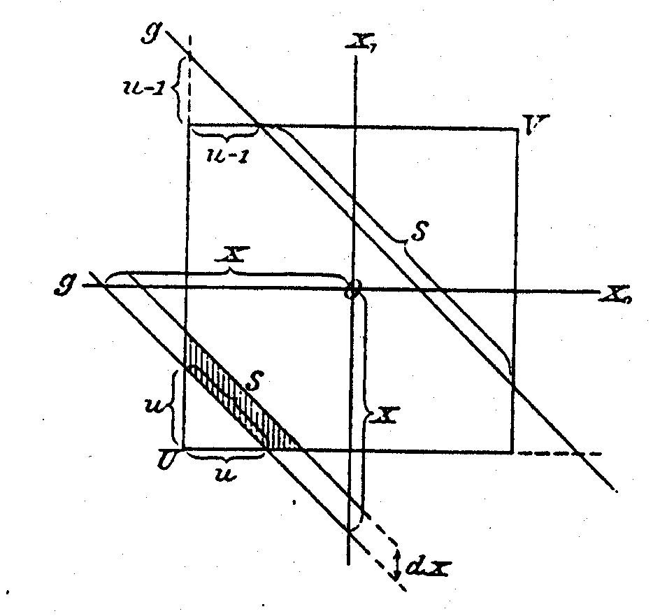
\includegraphics{figpage36.png} — Figure 3 $M_{2}$ - the piecewise linear case for $X_{1} + X_{2}$ .

We have already covered $M_{1}$ , so we can continue with $M_{2}$ , i.e., the sum $X_{1} + X_{2}$ . Figure 3 is taken directly from Sommerfeld’s paper. Working in $R_{2}$ with axes $x_{1}$ and $x_{2}$ , all possible outcomes for $X_{1}$ and $X_{2}$ are represented by pairs of numbers lying in a unit square centered at the origin, i.e., $Q_{2} = [- \frac{1}{2}, \frac{1}{2}] \times [- \frac{1}{2}, \frac{1}{2}]$ . All outcomes $(x_{1}, x_{2})$ resulting in the same sum $x$ lie on the line $x_{1} + x_{2} = x$ . Anyway, for small $d x > 0$ (the negative case is handled analogously) we are looking for the area of the region cut out of the square $Q_{2}$ by the strip $S (x, x + d x)$ between the two lines $x_{1} + x_{2} = x$ and $x_{1} + x_{2} = x + d x$ in the sense that

P (x \leq X_{1} + X_{2} \leq x + d x) = \int_{x}^{x + d x} M_{2} (t) d t = area (Q_{2} \cap S_{2} (x, x + d x)) .

The width of the strip $S (x, x + d x)$ as the distance between the two lines is $d x / \sqrt{2}$ , so that

area (Q_{2} \cap S_{2} (x, x + d x)) = \frac{1}{2} (S_{2} (x) + S_{2} (x + d x)) \frac{d x}{\sqrt{2}},

where $S_{2} (x)$ denotes the length of that part of the line $x_{1} + x_{2} = x$ which lies within the square $Q_{2}$ , since $Q_{2} \cap S_{2} (x, x + d x)$ is a trapezoid.

We obtain therefore that

\begin{aligned} M_{2} (x) & = lim_{d x \to 0} \frac{1}{d x} \int_{x}^{x + d x} M_{2} (t) d t \\ = lim_{d x \to 0} \frac{1}{2} (S_{2} (x) + S_{2} (x + d x)) \frac{1}{\sqrt{2}} = \frac{S_{2} (x)}{\sqrt{2}} . \end{aligned}

Thus our task is now reduced to finding a formula for $S_{2} (x)$ . The line intersects the square iff $- 1 \leq x < 1$ , so $S_{2} (x) = 0$ for $| x | \geq 1$ : To simplify we introduce $u = 1 + x$ , so that we still have to investigate the case $0 \leq u < 2$ . Note that $u$ is the distance from the corner of $(- \frac{1}{2}, - \frac{1}{2})$ of $Q_{2}$ to the point $(x + \frac{1}{2}, - \frac{1}{2})$ , where the line $x_{1} + x_{2} = x$ intersects the line containing that side of $Q_{2}$ , which originates at $(- \frac{1}{2}, \frac{1}{2})$ and is parallel to the $x_{1}$ -axis (the same for $(- \frac{1}{2}, x + \frac{1}{2})$ and the side parallel to the $x_{2}$ -axis).

For $0 \leq u < 1$ the point of intersection lies within $Q_{2}$ and so the right triangle with the vertices $(- \frac{1}{2}, - \frac{1}{2}), (x + \frac{1}{2}, - \frac{1}{2}),$ $(- \frac{1}{2}, x + \frac{1}{2})$ has a hypotenuse of length $S_{2} (x)$ and the other two sides are both of length $u$ . Thus by Pythagoras, since $S_{2} (x)$ is nonnegative:

{(S_{2} (x))}^{2} = 2 u^{2} \  or\ S_{2} (x) = \sqrt{2 u} = \sqrt{2} (1 + x) \  for - 1 \leq x < 0.

For $1 \leq u < 2$ the intersection point $(x + \frac{1}{2}, - \frac{1}{2})$ lies outside of $Q_{2}$ , so the length of the hypotenuse $\sqrt{2} u$ of the triangle with vertices $(- \frac{1}{2}, - \frac{1}{2}),$ $(x + \frac{1}{2}, - \frac{1}{2})$ and $(- \frac{1}{2}, x + \frac{1}{2})$ is in fact too long and we must subtract the length of the hypotenuses of the two small right triangles, one with vertices $(- \frac{1}{2}, \frac{1}{2}), (- \frac{1}{2}, x + \frac{1}{2})$ and $(x - \frac{1}{2}, \frac{1}{2})$ , the other with vertices $(\frac{1}{2}, - \frac{1}{2})$ , $(x + \frac{1}{2}, - \frac{1}{2})$ and $(\frac{1}{2}, x + \frac{1}{2})$ , whose other sides have both length $u - 1$ . This yields

S_{2} (x) = \sqrt{2} u - 2 \sqrt{2} (u - 1) = \sqrt{2} ((1 + x) - 2 x) = \sqrt{2} (1 - x), for 0 \leq x < 1,

so that we obtain, just as we should, $M_{2} (x) = \frac{S_{2} (x)}{\sqrt{2}} = N (x)$ .

We proceed now to $M_{3}$ and the sum $X_{1} + X_{2} + X_{3}$ . Again Figure 4 is the original one from Sommerfeld’s paper. Now the outcomes lie in the unit cube $Q_{3} = [- \frac{1}{2}, \frac{1}{2}) \times [- \frac{1}{2}, \frac{1}{2}) \times [- \frac{1}{2}, \frac{1}{2})$ and all outcomes with the same sum $x$ on the plane $x_{1} + x_{2} + x_{3} = x$ : Arguing as before for two variables, this time with the strip between the two planes for $x$ and $x + d x$ , we find that the strip has width $d x / \sqrt{3}$ and

M_{3} (x) = \frac{S_{3} (x)}{\sqrt{3}},

where $S_{3} (x)$ is the area of the piece of the plane $x_{1} + x_{2} + x_{3} = x$ that lies within the cube $Q_{3}$ . This time we have intersection iff $- \frac{3}{2} \leq x < \frac{3}{2}$ , so $S_{3} (x) = 0$ for $| x | \geq \frac{3}{2}$ . The substitution $u = \frac{3}{2} + x$ introduces again the length of the (now three) segments from the corner $(- \frac{1}{2}, - \frac{1}{2}, - \frac{1}{2})$ to the intersections of the lines containing a side of the cube originating at this corner with the plane $x_{1} + x_{2} + x_{3} = x$ .

\includegraphics[scale=1.2]{figpage38.jpg} — Figure 4 $M_{3}$ - the piecewise quadratic case for $X_{1} + X_{2} + X_{3}$ .

For $0 \leq u < 1$ these intersection points $(x + 1, - \frac{1}{2}, - \frac{1}{2}), (- \frac{1}{2}, x + 1, - \frac{1}{2})$ and $(- \frac{1}{2}, - \frac{1}{2}, x + 1)$ lie within the cube and $S_{3} (x)$ is the area of the equilateral triangle with these three vertices, so that its side length is $\sqrt{2} u$ and thus

S_{3} (x) = \frac{\sqrt{3}}{2} u^{2}, for 0 \leq u < 1.

For $1 \leq u < 2$ , the intersection is a hexagon, obtained from the triangle with vertices $(x + 1, - \frac{1}{2}, - \frac{1}{2}), (- \frac{1}{2}, x + 1, - \frac{1}{2}), (- \frac{1}{2}, - \frac{1}{2}, x + 1)$ by removing small equilateral triangles of length $\sqrt{2} (u - 1)$ at the corner, for example the one with the vertices $(x + 1, - \frac{1}{2}, - \frac{1}{2}), (- \frac{1}{2}, x, - \frac{1}{2}), (- \frac{1}{2}, - \frac{1}{2}, x)$ , yielding

S_{3} (x) = \frac{\sqrt{3}}{2} (u^{2} - 3 {(u - 1)}^{2}), for\ 1 \leq u < 2.

For $2 \leq u < 3$ , the intersection is again a triangle. Instead of computing its area directly, we observe that by taking away the triangles as we did for $1 \leq u < 2$ , we are now removing too much and have to add in again 3 triangles at each corner of side length $\sqrt{2} (u - 2)$ to obtain

S_{3} (x) = \frac{\sqrt{3}}{2} (u^{2} - 3 {(u - 1)}^{2} + 3 {(u - 2)}^{2}), \  for 2 \leq u < 3.

Finally, we consider $M_{3}$ and the sum $X_{1} + X_{2} + X_{3} + X_{4}$ . We find

M_{4} (x) = \frac{S_{4} (x)}{\sqrt{4}},

where $S_{4} (x)$ is the (3-dimensional) volume of the piece of the hyperplane $x_{1} + x_{2} + x_{3} + x_{4} = x$ that lies within the (4-dimensional) cube $Q_{4} = {[- \frac{1}{2}, \frac{1}{2})}^{4}$ . With the substitution $u = 2 + x$ , we obtain a regular tetrahedron as the intersection for $0 \leq u < 1$ , yielding

S_{4} (x) = \frac{\sqrt{4}}{6} u^{3}, for 0 \leq u < 1.

For $1 \leq u < 2$ , we obtain an octahedron, resulting from cutting four small tetrahedra at the 4 corners of the original tetrahedron, in order to get

S_{4} (x) = \frac{\sqrt{4}}{6} (u^{3} - 4 {(u - 1)}^{3}), \  for 1 \leq u < 2.

For $2 \leq u < 3$ , we still obtain an octahedron, but the four tetrahedra added in the previous step are overlapping now. As a compensation we have to add tetrahedra again, one for each edge of the original tetrahedron, i.e. a total of six to obtain

S_{4} (x) = \frac{\sqrt{4}}{6} (u^{3} - 4 {(u - 1)}^{3} + 6 {(u - 2)}^{3}), \  for 2 \leq u < 3.

Finally, for $3 \leq u < 4$ the intersection is a tetrahedron again, and we need to take away again a tetrahedron for each face of the original tetrahedron, so that

S_{4} (x) = \frac{\sqrt{4}}{6} (u^{3} - 4 {(u - 1)}^{3} + 6 {(u - 2)}^{3} - 4 {(u - 3)}^{3}), \  for 3 \leq u < 4.

A quick check shows that the function derived as $M_{4}$ is indeed the originally introduced $M_{4}$ and thus $B$ , establishing representation 2.16.

Sommerfeld was the first one (as far as I know) to present a graph of $B$ alias $M_{4}$ , together with those for $M_{1}, M_{2}$ and $M_{3}$ in his original paper from 1904, which is given in Figure 5, resolving item 2.17.

Note also that the formulae given for the pieces of the function $S_{4}$ are divided differences of the truncated power functions

S_{4} (x) = \frac{\sqrt{4}}{6} {[0, 1, 2, 3, 4]}_{t} {(u - t)}_{+}^{3},

yielding also

\begin{aligned} S_{4} (x) & = \frac{\sqrt{4}}{6} (u^{3} - 4 {(u - 1)}^{3} + 6 {(u - 2)}^{3} - 4 {(u - 3)}^{3} + {(u - 4)}^{3}) \\ = \frac{\sqrt{4}}{6} {[0, 1, 2, 3, 4]}_{t} (u - t)_{+}^{3} \frac{\sqrt{4}}{6} {[0, 1, 2, 3, 4]}_{t} {(u - t)}^{3} = 0, \  for u \geq 4. \end{aligned}

We will not sketch here how Sommerfeld pursued his original goal of investigating the limit behaviour, let it suffice to remark that indeed properly normalized B-splines tend to Gaussian (i.e., exponential) functions, if we let the polynomial degree go to infinity. Since Sommerfeld did not give a closed formula expression for his probability density functions $M_{n}$ , there were further attempts to shed some light on this problem, which did not become so widely known.

\includegraphics[scale=0.37]{fig_4_1.jpg} — Figure 5 Sommerfeld’s graphs for $M_{1}, M_{2}, M_{3}, M_{4} = B$ and the limit for $n \to \infty$ .

\includegraphics[scale=0.37]{fig_4_2.jpg} — Figure 5 Sommerfeld’s graphs for $M_{1}, M_{2}, M_{3}, M_{4} = B$ and the limit for $n \to \infty$ .

9 And something from Norway, too !

9.1 Brun 1932 (Item 2.18)

This section is devoted to the efforts of two Norwegian mathematicians, whose contributions and biographies are described in [ 7 ] . The first one is V. Brun, who is also the man who rediscovered Abel’s long lost original manuscript on transcendental functions, which Abel had submitted to the Academy in Paris in 1826. The text was finally printed in 1841, but the original was considered lost until Brun rediscovered it in Firenze in 1952. There were 8 pages missing, however, but that is another story, so back to our subject.

In his paper [ 6 ] in 1932, Brun had another look at the problem of the density functions $M_{n}$ as considered by Sommerfeld. He had the idea of relating these functions by an integral recursion corresponding to the convolution (6.9). He then found the following representation for $M_{1}$ : introducing the jump function

Q (x) = lim_{λ \to 0^{+}} \arctan (\frac{x}{λ}) = {\begin{cases} \frac{π}{2} & if x > 0, \\ 0 & if x = 0, \\ - \frac{π}{2} & if x < 0, \end{cases}

9.1

we have

Δ Q (x) = Q (x + \frac{1}{2}) - Q (x - \frac{1}{2}) = {\begin{cases} π if - \frac{1}{2} < x < \frac{1}{2}, \\ 0 if | x | > \frac{1}{2}, \\ \frac{π}{2} if x = \pm \frac{1}{2}, \end{cases}

so that $\frac{1}{π} Δ Q$ and $M_{1}$ only differ in the two points $\pm 1 / 2$ , which is irrelevant for integration, yielding

\frac{1}{π} \int_{x - \frac{1}{2}}^{x + \frac{1}{2}} Δ Q (t) d t = \int_{x - \frac{1}{2}}^{x + \frac{1}{2}} M_{1} (t) d t = M_{2} (x),

and thus by iteration

\frac{1}{π} \int_{x - \frac{1}{2}}^{x + \frac{1}{2}} \int_{t_{3} - \frac{1}{2}}^{t_{3} + \frac{1}{2}} \int_{t_{2} - \frac{1}{2}}^{t_{2} + \frac{1}{2}} Δ Q (t_{1}) d t_{1} d t_{2} d t_{3} = M_{4} (x),

i.e. representation 2.18. Brun then used $\frac{1}{π} Δ Q$ and the integral recursion to establish the functions $M_{n}$ in the integral form (6.10), and gave some quadrature formulae for the integration.

9.2 Fjelstaad 1937 (Items 2.19 and 2.20)

In his paper [ 6 ] , Brun stated: Vi ser herav det hpløse i fremstille $φ_{n} (x)$ efter potenser av $x$ (We see from here how hopeless it is to represent $φ_{n} (x)$ [his notation for $M_{n} (2 x)$ ] in powers of $x$ ). According to the introduction in [ 23 ] , this spurred on another Norwegian, J. E. Fjelstaad, to derive in fact such a representation from the integral form (6.10), bringing us to the end of our cubic B-spline tour.

Replacing $x$ by $x / 2$ we obtain from (6.10)

\begin{aligned} M_{n} (\frac{x}{2}) & = \frac{1}{π} \int_{0}^{+ \infty} {(\frac{\sin (\frac{ω}{2})}{\frac{ω}{2}})}^{n} \cos (\frac{x ω}{2}) d ω \\ = \frac{2}{π} \int_{0}^{+ \infty} {(\frac{\sin (ω)}{ω})}^{n} \cos (x ω) d ω . \end{aligned}

Integration by parts yields then formula

\frac{1}{3!} \int_{0}^{+ \infty} e^{- u ω} u^{3} d u = \frac{1}{ω^{4}},

so we obtain the double integral formula

\begin{aligned} M_{4} (\frac{x}{2}) & = \frac{2}{3! π} \int_{0}^{+ \infty} (\int_{0}^{+ \infty} e^{- u ω} u^{3} d u) \sin^{4} ω \cos (x ω) d ω \\ = \frac{2}{3! π} \int_{0}^{+ \infty} u^{3} (\int_{0}^{+ \infty} e^{- u ω} \sin^{4} ω \cos (x ω) d ω) d u . \end{aligned}

We compute that for the integral

I_{4} = \int_{0}^{+ \infty} e^{- (u - i x) ω} \sin^{4} ω d ω

we have

Re I_{4} = \int_{0}^{+ \infty} e^{- u ω} \sin^{4} ω \cos (x ω) d ω .

One integration by parts yields

I_{4} = \frac{4 \cdot 3}{4^{2} + {(u - i x)}^{2}} \int_{0}^{+ \infty} e^{- (u - i x) ω} \sin^{2} ω d ω

and yet another one

\begin{aligned} I_{4} & = \frac{4 \cdot 3}{4^{2} + {(u - i x)}^{2}} \frac{2 \cdot 1}{2^{2} + {(u - i x)}^{2}} \int_{0}^{+ \infty} e^{- (u - i x) ω} d ω \\ = \frac{4}{(4^{2} + {(u - i x)}^{2}) (2^{2} + {(u - i x)}^{2}) (u - i x)} . \end{aligned}

Thus we obtain

M_{4} (\frac{x}{2}) = \frac{8}{π} Re \int_{0}^{+ \infty} \frac{u^{3}}{(4^{2} + {(u - i x)}^{2}) (2^{2} + {(u - i x)}^{2}) (u - i x)} d u,

establishing item 2.19.

From here we want to proceed by using partial fractions. The zeros in the denominator are $i (x + 4 - 2 k)$ , $k = 0, 1, 2, 3, 4$ and we have

\frac{u^{3}}{\bigskip (4^{2} + {(u - i x)}^{2}) (2^{2} + {(u - i x)}^{2}) (u - i x)} = \sum_{k = 0}^{4} \frac{A_{k}}{u - i (x + 4 - 2 k)},

where the factors $A_{k}$ can be computed to be

\begin{aligned} A_{k} & = \frac{i^{3} {(x + 4 - 2 k)}^{3}}{\prod_{p = 0, p \neq k}^{4} (i (4 - 2 k) - i (4 - 2 p))} = - i \frac{{(x + 4 - 2 k)}^{3}}{\prod_{p = 0, p \neq k}^{4} (2 (p - k))} = - i \frac{{(x + 4 - 2 k)}^{3}}{{(- 1)}^{p} 2^{4} k! (4 - k)!} . \end{aligned}

Since

\sum_{k = 0}^{4} \frac{A_{k}}{u - i (x + 4 - 2 k)} = \sum_{k = 0}^{4} \frac{A_{k} (u + i (x + 4 - 2 k))}{u^{2} + {(x + 4 - 2 k)}^{2}},

we have

Re \sum_{k = 0}^{4} \frac{A_{k}}{u - i (x + 4 - 2 k)} = \sum_{k = 0}^{4} \frac{{(x + 4 - 2 k)}^{3}}{{(- 1)}^{p} 2^{4} k! (4 - k)!} \frac{(x + 4 - 2 k)}{u^{2} + {(x + 4 - 2 k)}^{2}} .

Integration from $0$ to $z$ yields

\int_{0}^{z} Re \sum_{k = 0}^{4} \frac{A_{k}}{u - i (x + 4 - 2 k)} d u = \sum_{k = 0}^{4} \frac{{(x + 4 - 2 k)}^{3}}{{(- 1)}^{k} 2^{4} k! (4 - k)!} \arctan (\frac{2}{x + 4 - 2 k}) .

Earlier we have already used limit properties of $\arctan$ in (9.4), here we see that

lim_{z \to \infty} \arctan (\frac{z}{x + 4 - 2 k}) = {\begin{matrix} \frac{π}{2}, if x + 4 - 2 k > 0, \\ - \frac{π}{2}, if x + 4 - 2 k < 0, \end{matrix}

so we finally establish

\begin{aligned} Re \int_{0}^{+ \infty} \sum_{k = 0}^{4} \frac{A_{k}}{u - i (x + 4 - 2 k)} d u = \\ = \frac{π}{2^{5}} \sum_{k = 0}^{4} \frac{{| x + 4 - 2 k |}^{3}}{{(- 1)}^{k} k! (4 - k)!} = \frac{π}{2^{5} 4!} \sum_{k = 0}^{4} {(- 1)}^{k} (\binom{4}{k}) {| x + 4 - 2 k |}^{3} \end{aligned}

and

M_{4} (\frac{x}{2}) = \frac{1}{3!} \frac{1}{2^{4}} \sum_{k = 0}^{4} {(- 1)}^{k} (\binom{4}{k}) {| x + 4 - 2 k |}^{3}

M_{4} (x) = \frac{1}{3!} \frac{1}{2^{4}} \sum_{k = 0}^{4} {(- 1)}^{k} (\binom{4}{k}) {| 2 x + 4 - 2 k |}^{3} = \frac{1}{3!} \frac{1}{2} \sum_{k = 0}^{4} {(- 1)}^{k} (\binom{4}{k}) {| x + 2 - k |}^{3},

establishing item 2.20. In the general case - which is of course the one considered in [ 23 ] , the signum function appears for odd polynomial orders (even degrees) in the sense that

M_{n} (x) = \frac{1}{(n - 1)!} \frac{1}{2} \sum_{k = 0}^{n} {(- 1)}^{k} (\binom{n}{k}) {| x + \frac{n}{2} - k |}^{n - 1} sign {(x + \frac{n}{2} - k)}^{n} .

10 An Outlook

A good way to wrap up our treatment now is to consider the general definition of a B-spline of arbitrary degree and make some comments in light of the 20 representations we have covered. For a more detailed introduction with examples and references I would like to refer to a recent tutorial [ 33 ] , standard spline monographs such as [ 3 ] , [ 42 ] and for the cardinal setting [ 40 ] , and specifically for CAGD [ 22 ] , [ 28 ] .

Schoenberg wrote his book [ 40 ] mainly about interpolation of infinite data by spline series of the form (4.1) for arbitrary polynomial degree. Still, in practical applications we regularly need to address situations with finitely many data points given over some finite interval, introducing the nontrivial problem of handling boundaries.

At first, let us check that divided differences can be defined recursively not just for simple distinct knots, but also for coalescing knots in the following way.

Definition 10.1

(Divided differences) Provided that a function $f$ is smooth enough so that all occurring derivatives are defined, the divided
difference of order $ℓ$ for the function $f$ in the points $t_{k} \leq \dots \leq t_{k + ℓ}$ is defined recursively as

[t_{k}] f = f (t_{k}), for\ ℓ = 0

and

[t_{k}, \dots, t_{k + ℓ}] f = {\begin{cases} \frac{[t_{k + 1}, \dots, t_{k + ℓ}] f - [t_{k}, \dots, t_{k + ℓ - 1}] f}{t_{k + ℓ} - t_{k}}, if t_{k} < t_{k + ℓ}, \\ \frac{f^{(ℓ)} (t_{k})}{ℓ!}, if t_{k} = \dots = t_{k + ℓ}, \end{cases} for ℓ \geq 1 .

We now start from a knot sequence $t$ of non-decreasing knots $t_{k}$ , which will serve as the breakpoints for the polynomial pieces

t : \dots \leq t_{k} \leq t_{k + 1} \leq \dots

To define B(asis)-splines of a given degree $d \geq 0$ , we need at least $d + 1$ knots and $t_{k} < t_{k + d + 1}$ for all possible $k$ to avoid functions identically zero.

Definition 10.2

(B-spline) For a given knot sequence $t$ the $k$ -th
B-spline of degree $d$ is defined as the divided difference with respect to $y$ of the truncated power function ${(y - x)}_{+}^{d}$ in the knots $t_{k}, \dots, t_{k + d + 1}$ , multiplied by the distance of the last and first knot in this subsequence, i.e.,

B_{k, d, t} (x) = B_{k, d} (x) = (t_{k + d + 1} - t_{k}) {[t_{k}, \dots, t_{k + d + 1}]}_{y} {(y - x)}_{+}^{d} .

At this point we have to say a bit more about knot sequences. There are two main settings. One is a biinfinite sequence of simple knots $t_{k}, k \in Z$ , with the most common example being the integers. For this cardinal setting $t_{C} : t_{k} = k$ , we have of course

\begin{aligned} B_{- 2, t_{C}, 3} (x) & = M (x | - 2, - 1, 0, 1, 2) \\ = M_{4} (x) = 4 {[- 2, - 1, 0, 1, 2,]}_{t} {(t - x)}_{+}^{3} = B (x) \end{aligned}

The other main setting is a finite knot sequence for a closed and bounded interval $[a, b]$ , typically a standard so-called $(d + 1)$ -regular knot sequence where, with $n \geq d + 1$ ,

\begin{aligned} t : t_{1} \leq t_{2} \leq \dots \leq t_{n + d} \leq t_{n + d + 1}, \\ where t_{k} < t_{k + d + 1}, k = 1, \dots, n, \\ {\it i.e.}, the maximum multiplicity of any given knots is d + 1 \\ t_{1} = t_{1} = \dots = t_{d + 1} = 0, \\ t_{n + 1} = t_{n + 2} = \dots = t_{n + d + 1} = b, \\ {\it i.e.}, the multiplicity of the endpoints is exactly d + 1. \end{aligned}

It must be strongly emphasized – although here we have mostly looked at just one spline function $B$ – that it is the set of all B-splines over a knot sequence that is needed in applications, such as manipulating a curve or solving a differential equation by collocation.

Based on Leibniz’ formula for divided differences

[t_{j}, t_{j + 1}, \dots, t_{j + k}] (g \cdot h) = \sum_{ℓ = j}^{j + k} ([t_{j}, \dots, t_{j + ℓ}] g) ([t_{j + ℓ}, \dots, t_{j + k}] h) .

one can establish a general recursion for B-splines (see item 2.4). With the B-splines of the initial level $d = 0$ , i.e., piecewise constants, defined as

B_{k, 0} (x) = {\begin{cases} 1, if\ x \in [t_{k}, t_{k + 1}) \\ 0, if x \notin [t_{k}, t_{x + 1}) \end{cases}

we have the following recursion for $d \geq 1$

B_{k, t, d} (x) = \frac{x - t_{k}}{t_{k + d} - t_{k}} B_{k, t, d - 1} (x) + \frac{t_{k + d + 1} - x}{t_{k + d + 1} - t_{k + 1}} B_{k + 1, t, d - 1} (x)

10.1

and thus triangular schemes for the evaluation of splines of the form

\sum_{k} c_{k} B_{k, t, d} (x)

10.2

analogous to the one introduced in subsection 3.6.

The continuity of a function of the form (10.2) is more tricky to describe. If all knots are simple, the polynomial pieces are glued together with continuity $d - 1$ . For a multiple knot, i.e., a number which occurs repeatedly in the knot sequence, the continuity in this breakpoint is reduced by the multiplicity of the knot. For a more detailed discussion see [ 33 ] . The flexibility of different orders of smoothness in different breakpoints is especially important in curve design for CAD/CAM.

The divided difference formulation (see item 2.5) shows that each B-spline is a piecewise polynomial as a linear combination of truncated powers. One can establish by induction, using the recursion (10.1), that

sup B_{k, t, d} = [t_{k}, t_{k + d + 1}] \  and B_{k . t, d} > 0 for x \in (t_{k}, t_{k + d + 1}) .

Using Peano’s theorem as in item 2.7, we can derive that the integral of a B-spline is given as

\int_{- \infty}^{\infty} B_{k, t, d} (x) d x = \frac{t_{k + d + 1} - t_{k}}{d + 1}

Note that the normalization factor in the B-spline definition is chosen to achieve a partition of unity, and we must change it to $d + 1$ to get spline functions that qualify as probability density functions (item 2.15). Only in the cardinal case we get both properties at the same time.

As for item 2.2, we can show the basis property of the set of B-splines, namely that all piecewise polynomials of degree $d$ , with smoothness in the breakpoints prescribed by the knot multiplicities, can be written in the form (10.2). This allows us also to show that the B-splines have smallest support under the given smoothness requirements. Also as in item 2.2, we can derive that the monomials can be represented as sums of the form (10.2), with coefficients given in terms of symmetric functions. Specifically, one gets that the B-splines form a partition of unity. The necessary general tool to show polynomial representation is the so-called Marsden identity [ 31 ] .

General multivariate splines are often defined by considering polynomials pieces over polyhedral domains (in two dimensions typically triangles or quadrilaterals) and gluing these pieces together at common facets with a given order of smoothness [ 10 ] , [ 4 ] . The geometric interpretation in item 2.18 is considered as the starting point for the investigation of so-called box splines [ 4 ] as multivariate piecewise polynomials, see Chapter 4 of [ 32 ] for a historical account including some reprints of Schoenberg’s letters from the early days.

Alternatively to the approach of gluing polynomial pieces, an extremal property generalizing (3.11) from item 2.1 has been used to define multivariate spline functions as those functions interpolating given data in some points and minimizing among all such interpolants an integral expression involving second order derivatives. These so-called thin-plate splines, introduced by Duchon [ 17 ] , however, are no longer piecewise polynomials for higher dimensions. For introductions to this subject see for example [ 18 ] , [ 19 ] .

Another really interesting topic, related to item 2.1, is the placing of interpolation conditions in some $x$ -values, called nodes, which do not necessarily coincide with any knots (breakpoints), such that we have a unique interpolant for a given spline space. The fundamental result stems from [ 41 ] for Lagrange interpolation, was extended to Hermite and other settings in [ 29 ] , and is also related to Green’s functions as touched upon in item 2.6 [ 30 ] . The Schoenberg- Whitney theorem says that for a given B-spline basis, the evaluation matrix needed for interpolation is non-singular if and only if its entries on the main diagonal are positive, meaning that the value of the $k$ -th B-spline in the $k$ -th interpolation node is positive. I will not even think of going into details here, such as totally positive matrices, variation diminishing splines, etc., etc.

Your mission, if you decide to accept it, is to find out much more about splines and their applications. Good Luck !

Bibliography

1

C. de Boor, Best approximation properties of spline functions of odd degree, J. Math. Mech. 12 (1963), pp. 747–750. $\includegraphics[scale=0.1]{ext-link.png}$

2

C. de Boor, On calculating with B-splines, J. Approx. Theory 6 (1972), pp. 50–62. $\includegraphics[scale=0.1]{ext-link.png}$

3

C. de Boor, A practical guide to splines, Springer, New York, 1978.

4

C. de Boor, K. Höllig, and S. Riemenschneider, Box splines, Springer, New York, 1993.

5

C. de Boor and R.E. Lynch, On splines and their minimum properties, J. Math. Mech., 15 (1966), pp. 953–970. $\includegraphics[scale=0.1]{ext-link.png}$

6

V. Brun, Gauss’ fordelingslov, Norsk Matematisk Tidsskrift, 14 (1932), pp. 81–92.

7

P.L. Butzer, M. Schmidt and E.L. Stark, Observations on the history of central B-splines, Archive for History of Exact Sciences, 39 (1988), pp. 137–156. $\includegraphics[scale=0.1]{ext-link.png}$

8

A.S. Cavaretta, W. Dahmen and C.A. Micchelli, Stationary subdivision, Memoirs of AMS 93, 1991. $\includegraphics[scale=0.1]{ext-link.png}$

9

G.M. Chaikin, An algorithm for high-speed curve generation, Comp. Graphics and Image Proc. 3 (1974), pp. 346–349. $\includegraphics[scale=0.1]{ext-link.png}$

10

C.K. Chui, Multivariate Splines, CBMS 54, SIAM, Philadelphia, 1988. $\includegraphics[scale=0.1]{ext-link.png}$

11

C.K. Chui, An Introduction to Wavelets, Academic Press, Boston, 1992.

12

M.G. Cox, The numerical evaluation of B-splines. J. Inst. Math. Applics. 10 (1972), pp. 134–139. $\includegraphics[scale=0.1]{ext-link.png}$

13

H.B. Curry, and I.J. Schoenberg, On Polya frequency functions IV. The fundamental spline and their limits, J. d’Analyse Math. bf 17 (1966), pp. 71–107. $\includegraphics[scale=0.1]{ext-link.png}$

14

I. Daubechies, Ten Lectures on Wavelets, CBMS 61, SIAM, Philadelphia, 1992. $\includegraphics[scale=0.1]{ext-link.png}$

15

P. J. Davis, Interpolation and Approximation 2nd edition, Dover, New York, 1975 (originally published 1963).

16

T. DeRose, M. Kass, and T. Truong, Subdivision surfaces in character animation, Computer Graphics 32 (1998), pp. 85–94. $\includegraphics[scale=0.1]{ext-link.png}$

17

J. Duchon, J., Interpolation des fonctions de deux variables suivant le principe de la flexion des plaques minces, RAIRO Analyse numérique, 10 (1976), pp. 5–12.

18

N. Dyn, Interpolation of scattered data by radial functions, in Topics in Multivariate Approximation, C.K. Chui, L.L. Schumaker, and F.I. Utreras (eds), Academic Press, New York, 1987, pp. 47–61.

19

N. Dyn, Interpolation and approximation by radial and related functions, in Approximation Theory VI, Vol. 1, C.K. Chui, L.L. Schumaker, and J.D. Ward (eds.), Academic Press, New York, 1989, pp. 211–234.

20

N. Dyn, Analysis of convergence and smoothness by the formalism of Laurent polynomials, in Tutorials on Multiresolution in Geometric Modelling, A. Iske, E. Quak, and M.S. Floater (eds.), Springer, Heidelberg, 2002, pp. 51–68. $\includegraphics[scale=0.1]{ext-link.png}$

21

F. Eggenberger, and G. Polya, Über die Statistik verketteter Vorgänge, Z. Angew. Math. Mech. 1 (1923), pp. 279–289. $\includegraphics[scale=0.1]{ext-link.png}$

22

G. Farin, Curves and Surfaces for Computer-Aided Geometric Design, 4th edition, Academic Press, San Diego, 1998.

23

J.E. Fjelstaad, Bemerking til Viggo Brun: Gauss’ fordelingslov, Norsk Matematisk Tidsskrift 19 (1937), pp. 69–71.

24

B. Friedman, A simple urn model, Comm. Pure Appl. Math. 2 (1949), pp. 59–70. $\includegraphics[scale=0.1]{ext-link.png}$

25

R.N. Goldman, Urn models, approximations, and splines. J. Approx. Theory 54 (1988), pp. 1–66. $\includegraphics[scale=0.1]{ext-link.png}$

26

R.N. Goldman, Recursive Triangles, in Computation of Curves and Surfaces, W. Dahmen, M. Gasca and C. M. Micchelli (eds), Kluwer, Dordrecht, 1989, pp. 27–72. $\includegraphics[scale=0.1]{ext-link.png}$

27

J.C. Holladay, A smoothest curve approximation, Math. Tables Aid. Comput. 11 (1957), pp. 233–243. $\includegraphics[scale=0.1]{ext-link.png}$

28

J. Hoschek, and D. Lasser, Fundamentals of Computer Aided Geometric Design, AKPeters, Wellesley, 1993.

29

S. Karlin, and Z. Ziegler, Chebyshevian spline functions, SIAM J. Numer. Anal. 3(1966), pp. 514–543. $\includegraphics[scale=0.1]{ext-link.png}$

30

M.G. Krein, and G. Finkelstein, Sur les fonctions de Green completement non-negatives des operateurs differentiels ordinaires, Doklady Akad. Nauk. SSSR 24 (1939), pp. 202–223.

31

M.J. Marsden, An identity for spline functions with applications to variation-diminishing spline approximation, J. Approx Theory 3 (1970), pp. 7–49. $\includegraphics[scale=0.1]{ext-link.png}$

32

C.A. Micchelli, Mathematical Aspects of Geometric Modelling, CBMS 65, SIAM, Philadelphia, 1995.

33

E. Quak, Nonuniform B-splines and $B$ -wavelets, in Tutorials on Multiresolution in Geometric Modelling, A. Iske, E. Quak, and M.S. Floater (eds.), Springer, Heidelberg, 2002, pp. 101–146. $\includegraphics[scale=0.1]{ext-link.png}$

34

G. de Rham, Un peu de mathématique à propos d’une courbe plane, Elemente der Mathematik 2 (1947), pp. 73–76, pp. 89–97.

35

C. Runge, Über empirische Funktionen und die Interpolation zwischen äquidistanten Ordinaten, Z. f. Math. u. Phys. 46 (1901), pp. 224–243.

36

M.A. Sabin, The use of piecewise forms for the numerical representation of shape, Dissertation, Hungarian Academy of Sciences, 1977.

37

M.A. Sabin, Subdivision of box-splines; Eigenanalysis and artifacts of subdivision curves and surfaces, in Tutorials on Multiresolution in Geometric Modelling, A. Iske, E. Quak, and M. S. Floater (eds.), Springer, Heidelberg, 2002, pp. 3–23, pp. 69–92. $\includegraphics[scale=0.1]{ext-link.png}$

38

I.J. Schoenberg, Contributions to the problem of approximation of equidistant data by analytic functions, Part A: On the problem of smoothing or graduation. A first class of analytic approximation formulae. Part B: On the second problem of osculatory interpolation. A second class of analytic approximation formulae. Quart. Appl. Math. 4 (1946), pp. 45–99 and pp. 112–141.

39

I.J. Schoenberg, On spline functions, in Inequalities I, O. Shisha (ed.), Academic Press, New York, 1967.

40

I.J. Schoenberg, Cardinal Spline Interpolation, CBMS 12, SIAM, Philadelphia,
1973. $\includegraphics[scale=0.1]{ext-link.png}$

41

I.J. Schoenberg, and A. Whitney, On Pólya frequency functions III. The positivity of translation determinants with an application to the interpolation problem by spline curves, Trans. Amer. Math. Soc. 74 (1953), pp. 246–259.

42

L.L. Schumaker, Spline Functions: Basic Theory, Wiley, New York, 1981.

43

A. Sommerfeld, Eine besonders anschauliche Ableitung des Gaussischen Fehlergesetzes, in Festschrift Ludwig Boltzmann gewidmet zum 60.Geburtstage, 20. Februar 1904, Barth, Leipzig, 1904, pp. 848–859.

44

J.L. Walsh, J.H. Ahlberg and E.N. Nilson, Best approximation properties of the spline fit, J. Math. Mech. 11 (1962), pp. 225–234. $\includegraphics[scale=0.1]{ext-link.png}$

This work is licensed under a Creative Commons Attribution 4.0 International License.

About B-splines. Twenty answers to one question: What is the cubic B-spline for the knots -2,-1,0,1,2?

1 Introduction

2 Twenty choices

3 Prelude: why is a spline called a spline?

3.1 The complete cubic spline interpolant

3.2 An extremal property

3.3 This why a spline is called a spline

3.4 A special case (Item 2.1)

4 One possible definition and some properties

4.1 A definition of a cubic B-spline

4.2 An explicit formula (Item 2.2)

4.3 The basis property

4.4 Local reproduction of polynomials

4.5 Minimal support (Item 2.3)

4.6 A recursion formula (Item 2.4)

5 Enter: truncated power functions

5.1 A closed formula for B-splines (Item 2.5)

5.2 Green’s functions (Item 2.6)

5.3 Peano kernels (Item 2.7)

5.4 A geometric interpretation (Item 2.8)

6 Fourier transforms

6.1 The Fourier transform of the B-spline $B$ (Item 2.9)

6.2 Convolutions (Item 2.10)

6.3 A moving unit impulse (Item 2.11)

7 Subdivision

7.1 The refinement equation (Item 2.12)

7.2 Subdivision curves (Item 2.13)

8 Probability

8.1 An urn model (Item 2.14)

8.2 A probability density function (Item 2.15)

8.3 Sommerfeld’s approach in 1904 (Items 2.16 and 2.17)

9 And something from Norway, too !

9.1 Brun 1932 (Item 2.18)

9.2 Fjelstaad 1937 (Items 2.19 and 2.20)

10 An Outlook

Bibliography

Information

Indexing and abstracting

Publisher

About B-splines. Twenty answers to one question: What is the cubic B-spline for the knots -2,-1,0,1,2?

1 Introduction

2 Twenty choices

3 Prelude: why is a spline called a spline?

3.1 The complete cubic spline interpolant

3.2 An extremal property

3.3 This why a spline is called a spline

3.4 A special case (Item 2.1)

4 One possible definition and some properties

4.1 A definition of a cubic B-spline

4.2 An explicit formula (Item 2.2)

4.3 The basis property

4.4 Local reproduction of polynomials

4.5 Minimal support (Item 2.3)

4.6 A recursion formula (Item 2.4)

5 Enter: truncated power functions

5.1 A closed formula for B-splines (Item 2.5)

5.2 Green’s functions (Item 2.6)

5.3 Peano kernels (Item 2.7)

5.4 A geometric interpretation (Item 2.8)

6 Fourier transforms

6.1 The Fourier transform of the B-spline B (Item 2.9)

6.2 Convolutions (Item 2.10)

6.3 A moving unit impulse (Item 2.11)

7 Subdivision

7.1 The refinement equation (Item 2.12)

7.2 Subdivision curves (Item 2.13)

8 Probability

8.1 An urn model (Item 2.14)

8.2 A probability density function (Item 2.15)

8.3 Sommerfeld’s approach in 1904 (Items 2.16 and 2.17)

9 And something from Norway, too !

9.1 Brun 1932 (Item 2.18)

9.2 Fjelstaad 1937 (Items 2.19 and 2.20)

10 An Outlook

Bibliography

Information

Indexing and abstracting

Publisher

6.1 The Fourier transform of the B-spline $B$ (Item 2.9)