Influence of control parameters on the stabilization of an Euler-Bernoulli flexible beam
Abstract.
In this work, we numerically study the influence of control parameters on the stabilization of a flexible Euler-Bernoulli beam fixed at one end and subjected at the other end to a force control and a moment control proportional respectively to velocity and rotating velocity. First, we analyze the displacement stabilization and the asymptotic behavior of the beam energy using a stable numerical scheme, resulting from the Crank-Nicholson algorithm for time discretization and the finite element method based on the approximation by Hermite’s cubic polynomial functions, for discretization in space. Then, by means of the finite element method, we represent the spectrum of the operator associated with this beam problem and we carry out a qualitative study of the locus of the eigenvalues according to the positive control parameters. From these studies we conclude that rotating velocity control has more effect on the stabilization of the beam compared to velocity control. Finally, this result is confirmed by a sensitivity study on the control parameters involved in the stabilization of the beam.
Key words and phrases:
beam equation, finite element method, asymptotic stability.2005 Mathematics Subject Classification:
35B35, 65N30, 35B401. Introduction
Boundary feedback stabilization of systems modeled by an Euler-Bernoulli beam equation is an important area of research for engineers and mathematicians alike. Many mechanical systems, such as telecommunications antennas and flexible robot arms, can be modeled using Euler-Bernoulli beam equations. In order to control the asymptotic dynamic behavior of these systems, a control law is associated with them. The aim is to promote energy dissipation in order to stabilize the system within a reasonable time.
In our study, we consider a flexible Euler-Bernoulli beam fixed at one end and subjected, at the other end, to a force control in velocity and a moment control in rotational velocity. The beam satisfies the Euler-Bernoulli equation
with initial conditions
At the embedded end (0), we have the following boundary conditions
At the end , we apply a force control in velocity and a moment control in rotating velocity
Notice that these last two equations indicate that the bending moment (i.e. ) and lateral force (i.e. ) of the beam at the free end (), are respectively controlled by the feedback laws in rotating velocity and velocity . Also, we assume that , are two positive constants involved in the boundary controls.
Assembling this together, we obtain the mathematical problem
| (1) | |||||
| (2) | |||||
| (3) | |||||
| (4) |
where is the transverse deflection of the beam at position and time . Also, the bending stiffness function, mass density function and beam length are taken to be equal to unity.
In [2], the system (1)–(4) is formulated as an evolution problem and it is proven that this problem is well posed in the sense of C0-semigroups of contractions. Also, Mensah E. Patrice in [7], studies the spectrum of the differential operator appearing in the exponential stabilization of this system. By means of a numerical scheme obtained by the finite difference method, the author studies the locus of eigenvalues as a function of the positive feedback parameters and , carrying out a qualitative study of the position of the spectrum with respect to a vertical asymptote.
In the case of our study, the aim is to determine the influence of each control parameter on the stabilization of this beam system and, more importantly, to show which one has the greatest influence. This will enable us to calibrate these parameters appropriately, so as to stabilize the system more rapidly.
We begin by developing a numerical scheme equivalent to the system (1)–(4), using the Crank-Nicholson algorithm for discretization in time and the finite element method based on approximation by cubic Hermite functions for discretization in space (see e.g. [4], [8]). Using this numerical scheme, we graphically analyze the influence of the positive feedback parameters and on displacement stabilization and the asymptotic behavior of beam energy. Then, using the finite element method, we represent the spectrum of the differential operator associated with the system (1)–(4) in order to qualitatively describe the impact of the control parameters on the positioning of the spectrum and its asymptote. In this way, we can observe the effect of each parameter on the energy decay rate and stabilization of the system under study. Finally, the conclusions of these graphical analyses are confirmed by a sensitivity study on these control parameters.
2. Numerical approximation of the system (1)–(4).
Let and consider the space
with
where in superscript represents the transposition.
The system (1)–(4) can be written as the evolution problem
| (5) |
With , for all . Note that is a linear operator, with domain
| (6) | ||||
and defined by
| (7) |
2.1. Discretization
2.1.1. Time discretization.
Let be a strictly positive real. The interval is discretized into intervals of the same length . Then, at each moment , we note respectively
and the approximate values of and Thus, we have with .
Using the Crank-Nicholson scheme for the time discretization of the problem (5), we obtain the following system
| (8) |
Moreover, for all and the variational formulation of the problem (8), is written
| (9) |
2.1.2. Discretization in space.
For discretization in space, we use the finite element method with Hermite’s cubic polynomial functions.
First, let us subdivide the interval into intervals of the same length with and . On each node , we associate the approximate values of and its derivative at the point .
Thus, in the same way as in [5], consider the functions as reference functions, from which the polynomial functions, and , are constructed such that:
For
For
with
We thus obtain a -tuple which we simply denote in the following and which constitutes a basis of dimension of the interpolation space . With
Thus, we have
| (10) |
and
| (11) | ||||
| (12) | ||||
| (13) |
with respectively and , the approximate values of and
2.2. Stability of the numerical scheme
For all, fixed point with , let us set
| (15) |
Then, the system (14) can be written as the following vector equation:
| (16) |
By multiplying (16) by the inverse of the left matrix, we obtain:
| (17) |
Now, to determine the associated Von-Neumann stability condition, let us consider
| (18) |
The system (17) becomes
| (19) |
3. Effects of control parameters on beam stabilization
3.1. Stabilization in motion
For all , consider the matrices
denotes the unit matrix of order
For numerical simulations, we consider as initial conditions:
with
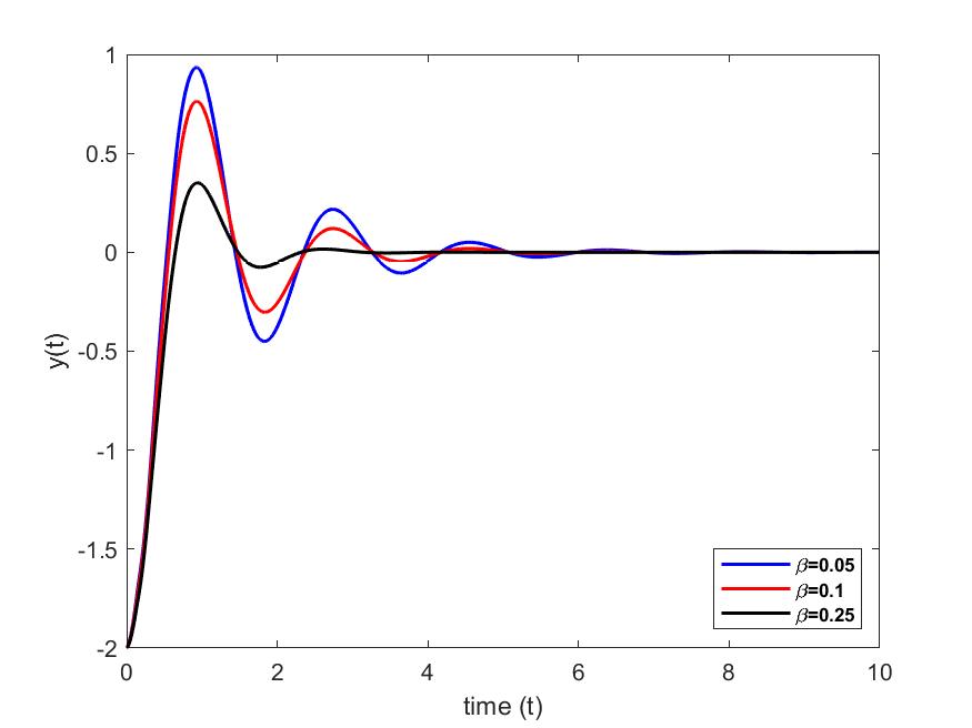
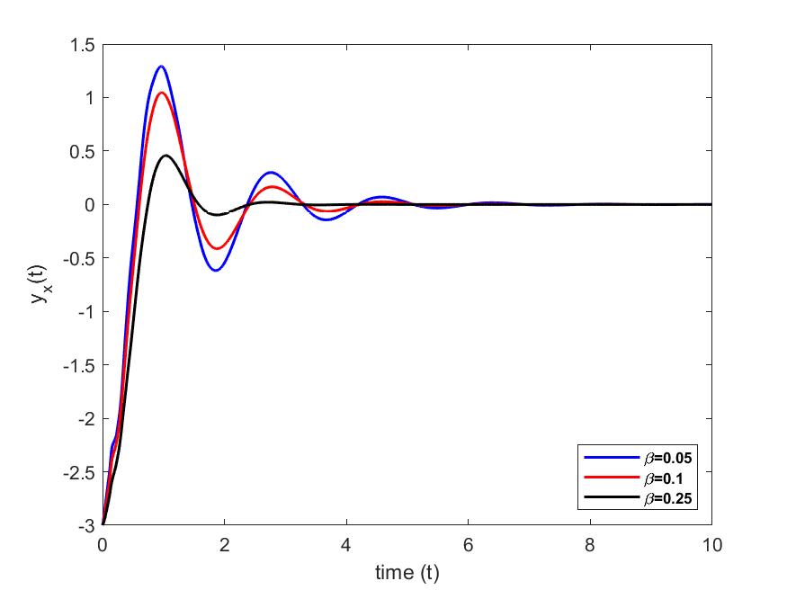
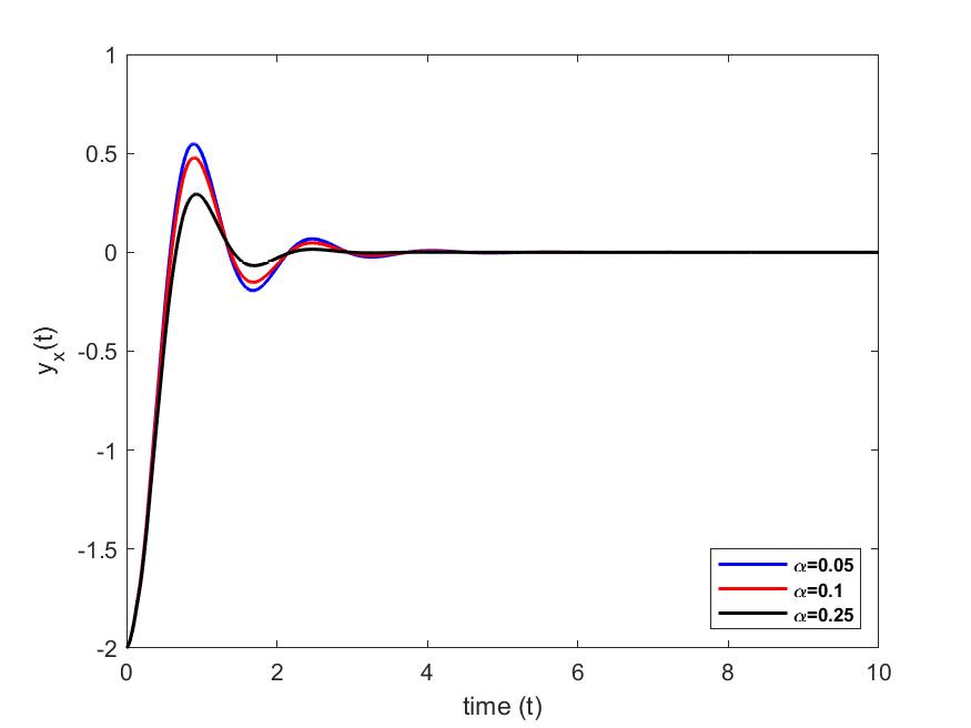
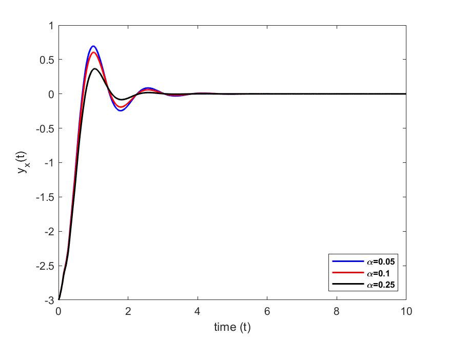
We represent the position and the angle of rotation of the beam at the free end (i.e. in ), for different values (taken arbitrarily) of the parameters and , in order to highlight their influences on the stabilization of the beam. The numerical simulations are carried out with MATLAB.
case 1: We set and we vary case 2: We set and we vary
3.2. Energy stabilization
Thus, the energy defines a Lyapunov function and satisfies .
Considering the Crank-Nicholson scheme, we have for the following discrete energy:
| (24) |
We then obtain the following result:
Proposition 1.
For any integer n, there is a positive real such that
| (25) |
Proof.
According to (24), we have
| (26) |
For , we replace in the first equation of the variational formulation (9), by . We obtain the following equation
| (27) |
Furthermore, considering as a test function in the second equation of the problem (9), we obtain the following equation:
| (28) | ||||
Analogously, if we choose as test function in the second equation of the system (9), we obtain:
| (29) | ||||
Therefore we have the following result:
Corollary 2.
For all we have
We notice that the energy of the discrete system decreases and is controlled by that of the initial data. From Proposition 1, we deduce the following equality:
| (33) |
, with
| (34) |
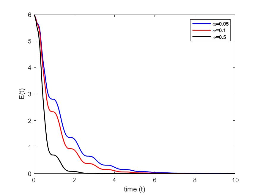
Now let us represent the energy of the system (1)–(4) for different values of and
case 1: We set and we vary
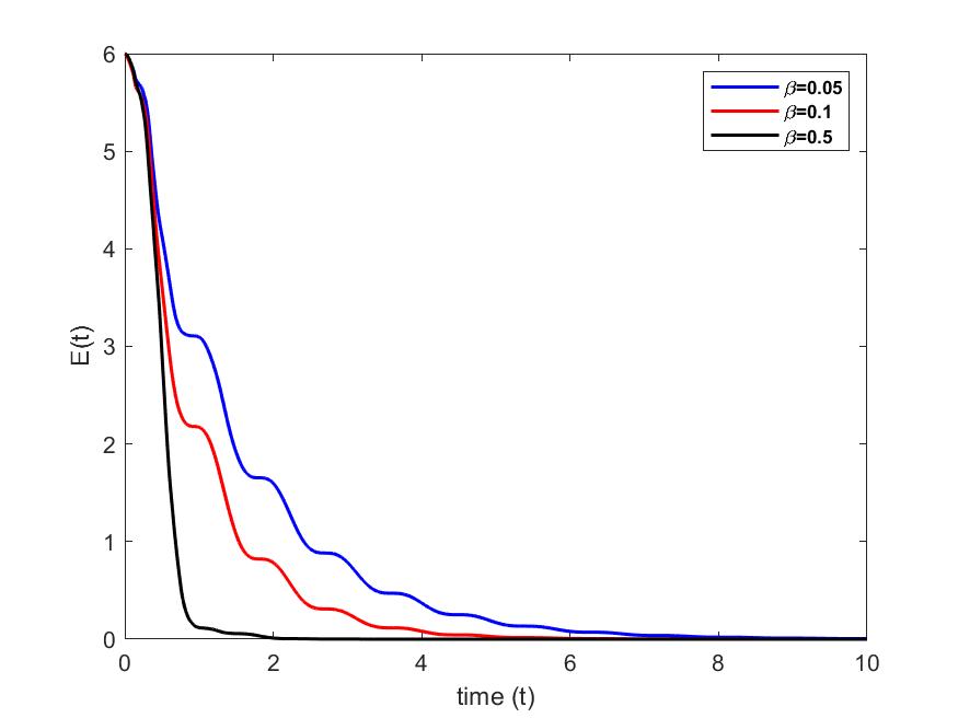
case 2: We set and we vary
3.3. Discussion of results
For a fixed value of and different values of , we see in Figs. 2 and 2 that vibrations at the free end of the beam cancel out at different times. In particular, they cancel faster as we increase the value of the parameter. However, for a fixed value of and for different values of , we see in Figs. 4 and 4 that vibrations at the free end of the beam cancel out at almost the same time. Furthermore, in Figs. 5 and 6, we see that when we increase the value of parameter , the energy decreases and cancels out faster than when the value of parameter is increased.
The moment control in rotation velocity therefore seems to have more impact on the stabilization of the beam and energy dissipation.
4. Influence of control parameters on the system spectrum.
To begin, let us recall the following theoretical result.
Theorem 3 ([7]).
Notice that is the vertical asymptote of the spectrum in the complex plane.
Recall that for the numerical study of the spectrum, we use the finite element method with the cubic polynomial functions of Hermite defined previously.
When we multiply the equation (1) by the test function , we obtain after two integrations by parts the following weak formulation:
| (36) |
Also, by separation of variables, the approximate solution in the base can be written as follows:
| (37) |
We denote , a vector representation of the function defined as follows:
Thus, the equation (36) becomes the following second order ordinary differential equation:
| (38) |
Let and . Then the equation (38) becomes with
the spectrum matrix.
Now, by implementing the spectrum matrix , we represent the spectrum of the system (1)–(4) for different values of and Note that for greater numerical precision, eigenvalues are calculated using the Advanpix multiprecision toolbox [3], quadruple precision (34 decimal digits) computation.
case 1: We set and we vary
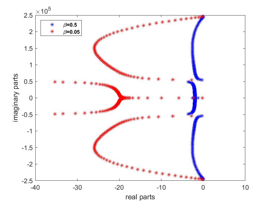

case 2: We set and we vary
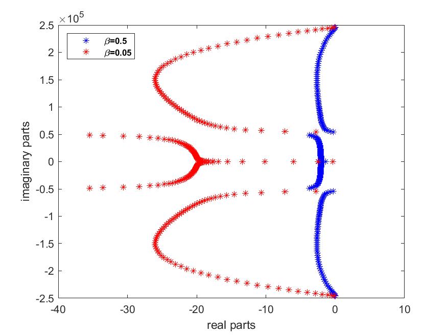
case 3: We set and we vary
4.1. Discussion of results
Numerical simulations of the spectrum have led to the following observations.
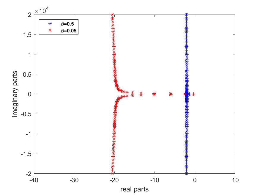
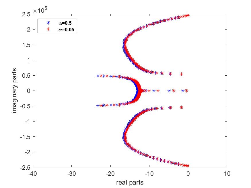
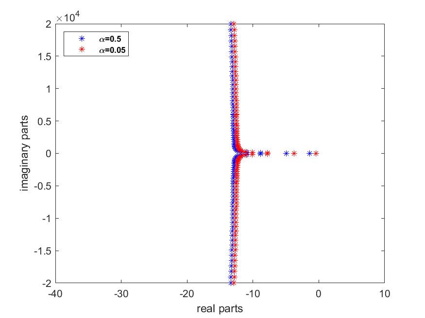
According to Figs. 10 and 10, for fixed values of , when we increase the value, the spectrum and asymptote shift significantly from left to right in the left complex half-plane. In addition, the number of low-frequency eigenvalues (those to the right of the asymptote ) decreases. It can therefore be said that significantly improves the energy decay rate and stability of the system.
However, Figs. 12 and 12 show that for a fixed value of , increasing the values of leads to a slight shift in the spectrum and asymptote of the left complex half-plane. In addition, the number of eigenvalues at low frequencies remains the same. This means that the parameter has little impact on the optimal energy decay rate and system stability.
We can therefore deduce that the moment control of the rotational velocity has a greater influence on the optimal rate of energy decay and the stability of the system
4.2. Sensitivity of Parameters and on the Stability
In this part, we objectively study the influence of the parameters and on the stabilization of the beam. So, for different values of and , we note in the table below, the damping time of the beam vibrations (i.e. time required to return to steady state ).
The first-order Sobol sensitivity [6] is written
| (39) |
where and ) represent respectively the variance of and the conditional expectation of obtained by setting and in (39).
| 0.8 | 1 | 5 | 10 | 15 | 20 | 30 | |
|---|---|---|---|---|---|---|---|
| 0.1 | 5.53 | 6.69 | 17.07 | 24.76 | 26.6 | 27.62 | 31.41 |
| 0.5 | 3.67 | 4.61 | 8.39 | 9.17 | 9.51 | 9.93 | 9.86 |
| 0.85 | 4.28 | 4.18 | 10.81 | 15.17 | 15.53 | 15.19 | 12.08 |
| 1 | 4.61 | 4.91 | 11.79 | 16.85 | 18.22 | 18.46 | 18.08 |
| 1.5 | 5.70 | 5.6 | 14.39 | 21.85 | 24.51 | 26.77 | 27.48 |
| 2 | 6.69 | 7.49 | 19.44 | 25.62 | 28.86 | 30.88 | 37.79 |
The calculation of the first order Sobol sensitivity indices gives us the following result:
According to the previous result, we have . We can deduce that the control parameter , has more impact on the stabilization of the beam compared to the parameter
5. Conclusion
In this work, we were interested in the influence of control parameters on the stabilization of a flexible Euler-Bernoulli beam, fixed at one end and subjected at the other end to a punctual force control and moment control proportional respectively to the velocity and the rotation velocity. We have developed a stable numerical scheme by means of which, we have shown by graphical analysis, that the moment control in rotation velocity has more influence on the stabilization of our model in displacement, in energy and on the positioning of the spectrum, in relation to the force control in velocity . This result was then confirmed by a statistical study of the sensitivity of the control parameters.
References
- [1] A.P. Abro Goh, G.J.M. Bomisso, K.A. Touré, Coulibaly Adama, A numerical study for a flexible Euler-Bernoulli beam with a force control in velocity and a moment control in rotating velocity, J. Indian Math. Soc., 90 (2023), pp. 125–148. https://doi.org/10.18311/jims/2023/3304
- [2] Advanpix, Multiprecision Computing Toolbox for MATLAB.
- [3] P.Z. Bar-Yoseph, D. Fisher, O. Gottlieb Spectral element methods for nonlinear spatio-temporal dynamics of an Euler-Bernoulli beam, Comput. Mech., 19 (1996), pp. 136–151. https://doi.org/10.1007/bf02824851
- [4] H. Laousy, On some problems of stabilization of systems with distributed parameters, Doctoral thesis, Paul Verlaine University, Metz, (1997). https://doi.org/10.1051/COCV:200206
- [5] M.D. McKay, Evaluating prediction uncertainty, Technical Report NUREG/CR-6311, US Nuclear Regulator Commission and Los Alamos National Laboratory, New Mexico, NM, USA, (1995).
- [6] Mensah E. Patrice, On the numerical approximation of the spectrum of a flexible Euler-Bernoulli beam with a force control in velocity and a moment control in rotating velocity, Far East J. Math. Sci., 126 (2020), pp. 13–31. http://dx.doi.org/10.17654/MS126010013.
- [7] I.H. Shames, C. Dym, Energy and Finite Element Methods in Structural Mechanics, New Age International (P) Ltd., (1995).


