Iterative schemes for coupled flow and transport
in porous media - Convergence and truncation errors

Abstract.

Nonlinearities of coupled flow and transport problems for partially saturated porous media are solved with explicit iterative $L$-schemes. Their behavior is analyzed with the aid of the computational orders of convergence. This approach allows highlighting the influence of the truncation errors in the numerical schemes on the convergence of the iterations. Further, by using manufactured exact solutions, error-based orders of convergence of the iterative schemes are assessed and the convergence of the numerical solutions is demonstrated numerically through grid-convergence tests.

1. Introduction

Flow and reactive transport in porous media are modeled by systems of coupled nonlinear partial differential equations. The seepage velocity through the bulk of porous medium is proportional to the hydraulic conductivity and to the gradient of the pressure head, according to Darcy’s law, which combined with the conservation equation results in the Richards’ equation. In its general, mixed formulation, Richards’ equation contains two unknown functions, the volumetric water content and the pressure head. Therefore, it needs to be closed by constitutive relationships for the dependence of the water content on the pressure head and the dependence of the hydraulic conductivity on the water content. Such relationships are highly nonlinear, e.g., the exponential model or the van Genuchten-Mualem model, with discontinuous derivatives when the negative pressure, in unsaturated flow regime, changes into the positive pressure characterizing the saturated regime with constant water content and hydraulic conductivity. Consequently, the resulting Richards’ equation for the pressure head is non-linear and parabolic-elliptic degenerate.

The concentration of the chemical compounds transported in soils and aquifers is governed by parabolic advection-diffusion-reaction equations, with flow velocity provided by the solution of the Richards’ equation. In the presence of capillarity effects, for instance in problems of surfactant transport, the water content depends on pressure as well as on concentration and the flow and transport equations are coupled in a nonlinear way in both directions. Solving these coupled nonlinear problems requires iterative schemes that use different linearization techniques, such as Newton’s method, (modified) Picard method, $L$-scheme or their combinations. While Newton’s method is second order (under usual circumstances) but only locally convergent, which means that it converges only if the initial choice is not too far from the solution, the $L$-scheme is a robust method unconditionally first order convergent, the robustness of the Picard method being somewhere in between [8]. A significant improvement of the convergence can be achieved by starting with $L$-scheme iterations and, once an appropriate initial solution is found, switching to the faster and higher order convergent Newton’s method [13].

The $L$-scheme can be thought as a quasi-Newton method, with derivative of the water content with respect of the pressure head replaced by a positive constant $L$. This makes it robust and independent of the initial choice, at the price of being only first order convergent. Given its simplicity, the $L$-scheme is particularly suitable in solving intricate and fully coupled nonlinear problems. Most of the implementations of the $L$-scheme are implicit linearizations based on finite element [9, 8, 13] or finite volume [10, 5] discretizations. Explicit $L$-schemes based on finite difference (FD) and random walk methods, introduced in [17], have been successfully used to solve coupled problems of flow and biodegradation in partially saturated soils and saturated heterogeneous aquifers [18]. The reason of using explicit $L$-schemes is that numerical solutions of the flow equations are obtained on the same regular grid on which reactive transport is solved with random walk algorithms free of numerical diffusion [17].

Theoretical proofs of convergence of the linearization schemes essentially show that the errors of the iterative solutions with respect to the exact solution of the nonlinear problem can be made arbitrarily small [8]. However, even if the numerical analysis of the scheme provides estimates of the convergence rates, in general it does not produce a thorough and comprehensive characterization of the type of convergence behavior, by predicting the upper/lower limits of the rates as in the theory of the convergent sequences [3, 4]. The analysis can be completed either by assessing computational orders of convergence, with sequences of successive corrections, or by assessing error-based orders, when exact solutions of the problem are available [20]. This approach could be mainly useful when the constraints required by the theoretical proofs are hard to meet, or when there are no convergence proofs at all, but, in practice, the convergence of the scheme is demonstrated numerically.

We investigate in this framework the convergence of the explicit $L$-scheme through computational and error-based orders of convergence on three numerical examples: solutions of Richards’ equation, fully coupled flow and surfactant transport, and coupled flow and transport with van Genuchten-Mualem parametrization.

2. Coupled flow and transport in porous media

We consider in the following the fully coupled one-dimensional problem of flow governed by Richards’ equation and transport of a single chemical species governed by an advection-diffusion-reaction equation,

(1) $$\frac{\partial }{\partial t}\theta (\psi ,c)-\frac{\partial }{\partial z}\left[K(\theta (\psi ,c))\frac{\partial }{\partial z}(\psi +z)\right]=0,$$

(2) $$\frac{\partial }{\partial t}\left[\theta (\psi ,c)c\right]-\frac{\partial }{\partial z}\left[D\frac{\partial }{\partial z}c-qc\right]=R(c),$$

where $\psi (z,t)$ is the pressure head, with $z$ being the height against the gravitational direction, $\theta$ is the water content, $q=-K(\theta (\psi ,c))\frac{\partial }{\partial z}(\psi +z)$ is the water flux (also called Darcy velocity), $K$ stands for the hydraulic conductivity of the porous medium, $c$ is the concentration, $D$ is the diffusion/dispersion coefficient, and $R$ is the reaction term. The system (1)-(2) is closed via constitutive relationships defining the dependencies $\theta (\psi ,c)$ and $K(\theta (\psi ,c))$.

Equations (1)-(2) are fully coupled through the terms $\theta (\psi ,c)$ and $[\theta (\psi ,c)c]$. Richards’ equation (1) is parabolic-elliptic degenerate, with variable $\theta (\psi ,c)$ if and $\theta =const$ if $\psi \ge 0$. Since the system is strongly nonlinear, through the functional dependencies $\theta (\psi ,c)$ and $K(\theta (\psi ,c))$, linearization methods have to be used to compute numerical solutions.

2.1. Explicit $L$-schemes for one-dimensional Richards’ equation

Following [17], we start with the staggered FD scheme with backward discretization in time of the Richards’ equation (1) decoupled from the transport equation (2),

$\theta ({\psi }_{i,k})-\theta ({\psi }_{i,k-1})=$

$=\frac{\mathrm{\Delta }t}{\mathrm{\Delta }{z}^2}\{[K(\theta ({\psi }_{i+1/2,k}))({\psi }_{i+1,k}-{\psi }_{i,k})-K(\theta ({\psi }_{i-1/2,k}))({\psi }_{i,k}-{\psi }_{i-1,k})]$

(3) $+(K(\theta ({\psi }_{i+1/2,k}))-K(\theta ({\psi }_{i-1/2,k})))\mathrm{\Delta }z\}.$

To obtain an iterative method for solving Richard’s equation, we denote by ${\psi }_{i,k}^s$ the approximate solution after $s$ iterations and add to the l.h.s. a stabilization term $L({\psi }_{i,k}^{s+1}-{\psi }_{i,k}^s)$, where $L$ is a constant which has the dimension of an inverse length. Whenever the iterative method converges, this stabilization term vanishes and the limit is the solution of the nonlinear scheme (2.1). Defining the dimensionless numbers $r_{i\pm 1/2,k}^s=K({\psi }_{i\pm 1/2,k}^s)\mathrm{\Delta }t/(L\mathrm{\Delta }{z}^2)$, one obtains

${\psi }_{i,k}^{s+1}=[1-(r_{i+1/2,k}^s+r_{i-1/2,k}^s)]{\psi }_{i,k}^s+r_{i+1/2,k}^s{\psi }_{i+1,k}^s+r_{i-1/2,k}^s{\psi }_{i-1,k}^s$

(4) $+(r_{i+1/2,k}^s-r_{i-1/2,k}^s)\mathrm{\Delta }z-(\theta ({\psi }_{i,k}^s)-\theta ({\psi }_{i,k-1}))/L.$

In practice, we run successive iterations $s=1,2,\mathrm{\dots }$ until a threshold condition is fulfilled, e.g., $\Vert {𝝍}_k^s-{𝝍}_k^{s-1}\Vert \le {\epsilon }_a+{\epsilon }_r\Vert {𝝍}_k^s\Vert$, where ${𝝍}_k^s$ denotes the solution vector of components ${\psi }_{i,k}^s$, $i=1,\mathrm{\dots },I$, $\parallel \cdot \parallel$ is the $l^2$ norm, and ${\epsilon }_a\ge 0$ and ${\epsilon }_r\ge 0$ are the absolute and relative tolerances (see e.g., [8]). The relation (2.1) is an explicit $L$-scheme that allows the computation of the approximate solution recursively and avoids the need to solve systems of linear equations, as in implicit finite element [8] or finite volume [10] $L$-schemes. Consequently, the explicit scheme (2.1) vas found to be one order of magnitude faster than the implicit finite volume $L$-scheme when solving typical problems for partially saturated flows [17].

To transform the FD scheme (2.1) into a random walk scheme we represent the solution ${\psi }_{i,,k}^s$ by $𝒩$ particles distributed over the lattice sites, ${\psi }_{i,k}^s\approx n_{i,k}^{s}a/𝒩$, where $a$ is a unit length that will be disregarded in the following. This results in the following relation summing contributions from neighboring sites to the number of particles at the site $i$ and time step $k$,

(5) $$n_{i,k}^{s+1}=\left[1-(r_{i+1/2,k}^s+r_{i-1/2,k}^s)\right]n_{i,k}^s+r_{i+1/2,k}^s{n}_{i+1,k}^s+r_{i-1/2,k}^s{n}_{i-1,k}^s+\lfloor 𝒩f^s\rfloor ,$$

where $f^s=(r_{i+1/2,k}^s-r_{i-1/2,k}^s)\mathrm{\Delta }z-[\theta (n_{i,k}^s)-\theta (n_{i,k-1})]/L$ and $\lfloor \cdot \rfloor$ is the floor function.

In order for (5) to be a random walk scheme, the coefficients multiplying numbers of particles at lattice sites $[1-(r_{i+1/2,k}^s+r_{i-1/2,k}^s)]$, $r_{i+1/2,k}$, and $r_{i-1/2,k}$ should be normalized probabilities. This implies the following restriction $[1-(r_{i+1/2,k}^s+r_{i-1/2,k}^s)]\le 1$. A sufficient condition for that is

(6) $$r_{i\pm 1/2,k}^s\le 1/2.$$

The first three terms in r.h.s. of (5) represent groups of particles jumping on the site $i$ form the right and from the left, and the ratio of the initial number of particles at the site $i$ which do not undergo jumps,

(7) $$\delta n_{i\mid i\pm 1,k}=r_{i\pm 1/2,k}^s{n}_{i\pm 1,k}^s,\delta n_{i\mid i,k}=\left[1-(r_{i+1/2,k}^s+r_{i-1/2,k}^s)\right]n_{i,k}^s.$$

With (7), (5) becomes

(8) $$n_{i,k}^{s+1}=\delta n_{i\mid i,k}+\delta n_{i\mid i+1,k}+\delta n_{i\mid i-1,k}+\lfloor 𝒩f^s\rfloor .$$

The numbers $\delta n$ of random walkers are binomially distributed random variables. Unlike in classical random walk approaches, consisting of generating random walk trajectories and counting particles at lattice sites, we directly evaluate the binomial variables $\delta n$ and construct a global random walk (GRW) [22]. Since there are different probabilities $r_{j\pm 1/2,k}$ for the right/left jumps, one obtains a biased global random walk (BGRW) [15]. The resulting BGRW algorithm moves the particles from a given lattice site $j$ according to the rule

(9) $$n_{j,k}^s=\delta n_{j\mid j,k}^s+\delta n_{j+1\mid j,k}^s+\delta n_{j-1\mid j,k}^s,$$

where

(10) $$\delta n_{j\pm 1\mid j,k}=r_{j\pm 1/2,k}^s{n}_{j,k}^s,\delta n_{i\mid i,k}=[1-(r_{j+1/2,k}^s+r_{j-1/2,k}^s)]n_{i,k}^s.$$

The random variable $\delta n_{j+1\mid j,k}=r_{j+1/2,k}^s{n}_{j,k}^s$ representing the number of right jumps in (9) is binomially distributed, with parameters $n_{j,k}^s$, $p=r_{j+1/2,k}^s/r_{i,k}^s$, and $q=1-p=r_{j-1/2,k}^s/r_{i,k}^s$, where $r_{i,k}^s=r_{j+1/2,k}^s+r_{j-1/2,k}^s$. The number of left jumps is the difference between the total number of jumps and the number of right jumps $\delta n_{j-1\mid j,k}=r_{i,k}^s{n}_{j,k}^s-\delta n_{j+1\mid j,k}$. Since the computation of the exact binomial distribution could be computationally prohibitive for very large $n_{j,k}^s$, one uses its approximation via a “reduced-fluctuations algorithm” similar to that proposed for the unbiased GRW algorithm in [22] as follows:

algorithm 1.

Reduced fluctuations algorithm
(i) initialize a real variable $rest=0$;
(ii) compute $\delta n$ with the relations (10);
(iii) split $\delta n$ into $\delta n=\lfloor \delta n\rfloor +\{\delta \}$ at every lattice site;
(iv) approximate $\delta n$ by $\lfloor \delta n\rfloor$;
(v) sum up the remainders into the variable $rest=\sum \{\delta \}$ over all the sites;
(vi) allocate one particle to the first lattice site where $rest\ge 1$;
(vii) save $rest=rest-1$ and repeat the sequence (ii)-(vi) at every $k$.

Specifically, the algorithm is implemented in the Matlab code as follows:

Code 1.

Flow-BGRW with reduced fluctuations

restr=0; rest1=0; rest2=0;
D=K(tht); D=D(1:I-1); % conductivity function of water content
r=dt*D/dx^2/L;
rloc=[1-2*r(1),1-(r(1:I-2)+r(2:I-1)),1-2*r(I-1)];
restr=rloc.*n+restr; nn=floor(restr); restr=restr-nn;
rest1=r(2:I-1).*n(3:I)+rest1;
njumpleft=floor(rest1); rest1=rest1-njumpleft; % left jumps
nn(2:I-1)=nn(2:I-1)+njumpleft;
rest2=r(1:I-2).*n(1:I-2)+rest2;
njumpright=floor(rest2); rest2=rest2-njumpright; % right jumps
nn(2:I-1)=nn(2:I-1)+njumpright;

1 computes the solution in the interior of the domain. The Darcy velocity on the boundaries can be computed in several ways: using an approximate forward finite difference discretization of Darcy’s law, extending on the boundary the velocity from the first neighboring interior site, computing the exact velocity analytically when a manufactured solution for the pressure head is available [17, Sect. 5.2.1].

Remark 1.

Since the BGRW is an explicit scheme, the source term can be evaluated first, then the first tree terms of (8) which model the transport will be computed according to 1. The reduced-fluctuations algorithm preserves the indivisibility of the particles by summing up to unity the fractional parts $\{\cdot \}$ of all the terms defined by (7). Therefore, the floor function in (8) is no longer necessary and the source term becomes $𝒩f^s$. Dividing (8) by $𝒩$, using (7), and taking the average, one retrieves the FD $L$-scheme (2.1) for the unknown ${\psi }_{i,k}^s=\overline{n_{i,k}^s}/𝒩$. A condition of kind $K\mathrm{\Delta }t/\mathrm{\Delta }{z}^2\le 1/2$ ensures the stability of the forward-time central-space scheme for the heat equation with constant coefficient $K$ and is assumed (without carrying out the stability analysis) to hold in case of variable coefficients as well [14]. In the present context, the condition (6) guaranties that particles cannot be created or destroyed otherwise than through boundary conditions or in the presence of an internal source/sink, that is, it ensures the stability of the BGRW $L$-scheme (5). Since the FD $L$-scheme (2.1) is the ensemble average of the BGRW scheme, its stability is also ensured by the constraint (6).

The FD scheme is also retrieved when all floor operators are removed in 1. The resulting code sequence can be recast as the FD scheme presented in 2 below, where $p=n/𝒩$ and $pp=nn/𝒩$.

Code 2.

Flow-FD scheme

D=K(tht); D=D(1:I-1); % conductivity function of water content
r=dt*D/dx^2/L;
rloc=[1-2*r(1),1-(r(1:I-2)+r(2:I-1)),1-2*r(I-1)];
pp=rloc.*p;
pp(2:I-1)=pp(2:I-1)+r(2:I-1).*p(3:I)+r(1:I-2).*p(1:I-2);

Remark 2.

In the particular case of the saturated regime, $\theta =const$, with space-variable hydraulic conductivity $K$ and a given source term $f$, after setting $L=1$ and disregarding the time index $k$ in (2.1) one obtains a transient scheme to solve the equation for the hydraulic head $h=\psi +z$,

$$\frac{1}{a}\frac{\partial h}{\partial s}-\frac{\partial }{\partial z}\left[K\frac{\partial h}{\partial z}\right]=f.$$

This scheme has been used to solve coupled flow and transport in saturated aquifers with moderate heterogeneity [16]. However, because the transient scheme may be very slow for highly heterogeneous coefficients $K$ [2], a more efficient strategy to solve coupled problems for saturated porous media is the coupling between an implicit FD flow scheme [2] and a GRW transport solver, see https://github.com/PMFlow/Coupled_FDM_GRW.

Matlab codes for one- and two-dimensional solutions of Richards’ equation, verification tests, and benchmark problems presented in [17] are posted at https://github.com/PMFlow/RichardsEquation.

2.2. Explicit BGRW scheme for reactive transport

Similarly to the derivation of the flow scheme in Section 2.1, we start with a FD scheme with backward time discretization of the equation (2) with a constant diffusion coefficient $D$,

$\theta ({\psi }_{i,k},c_{i,k})c_{i,k}-\theta ({\psi }_{i,k-1},c_{i,k-1})c_{i,k-1}=-$

$=-tfrac\mathrm{\Delta }t2\mathrm{\Delta }z(q_{i+1,k}{c}_{i+1,k}-q_{i-1,k}{c}_{i-1,k})+\frac{D\mathrm{\Delta }t}{\mathrm{\Delta }{z}^2}(c_{i+1,k}-2c_{i,k}+c_{i-1,k})+R(c_{i,k})=$

(11) $-\frac{2D\mathrm{\Delta }t}{\mathrm{\Delta }{z}^2}{c}_{i,k}+\left(\frac{D\mathrm{\Delta }t}{\mathrm{\Delta }{z}^2}-\frac{\mathrm{\Delta }t}{2\mathrm{\Delta }z}{q}_{i+1,k}\right)c_{i+1,k}+\left(\frac{D\mathrm{\Delta }t}{\mathrm{\Delta }{z}^2}+\frac{\mathrm{\Delta }t}{2\mathrm{\Delta }z}{q}_{i-1,k}\right)c_{i-1,k}+\mathrm{\Delta }tR(c_{i,k}),$

where ${\psi }_{i,k}$ is the solution of the coupled flow solver. Further, we denote by $c_{i,k}^s$ the approximate solution after $s$ iterations, add to the l.h.s. of (2.2) a stabilization factor $L(c_{i,k}^{s+1}-c_{i,k}^s)$, where $L$ is now a dimensionless constant, and define the dimensionless parameters

(12) $$r=\frac{2D\mathrm{\Delta }t}{L\mathrm{\Delta }{z}^2},v_{i\pm 1,k}^s=\frac{\mathrm{\Delta }t}{L\mathrm{\Delta }z}{q}_{i\pm 1,k}^s.$$

Representing the concentration by the distribution of $𝒩$ particles on the lattice, $c_{i,k}^s\approx n_{i,k}^s/𝒩$, and using the parameters (12), the stabilized version of the scheme (2.2) becomes an explicit $L$-scheme,

(13) $n_{i,k}^{s+1}=(1-r)n_{i,k}^s+\frac{1}{2}(r-v_{i+1,k}^s)n_{i+1,k}^s+\frac{1}{2}(r+v_{i-1,k}^s)n_{i-1,k}^s+\lfloor g^s\rfloor ,$

where $g^s=𝒩\left\{\mathrm{\Delta }tR(n_{i,k}^s)/L-[\theta ({\psi }_{i,k}^s,n_{i,k}^s)n_{i,k}^s-\theta ({\psi }_{i,k-1},n_{i,k-1})n_{i,k-1}]/L\right\}$.

With the constrains

(14) $$r\le 1,|v_{i,k}^s|\le r,$$

which ensure the normalization of the jump probabilities, the explicit $L$-scheme (13) for reactive transport is defined as a BGRW algorithm. The gathering and the spreading of groups of particles at/from a lattice point are described by relations similar to (8) and (9). The binomial random variables $\delta n$ are defined by

(15) $$\delta n_{j\pm 1\mid j,k}^s=\frac{1}{2}(r\pm v_{j,k}^s)n_{j,k}^s,\delta n_{j\mid j,k}^s=(1-r)n_{j,k}^s.$$

Remark 3.

The biased jump probabilities $\frac{1}{2}(r\pm v_{j,k}^s)$ in (15) simulate the advective displacement by moving larger numbers of particles in the positive flow direction. With an unbiased GRW, the advection is simulated by moving groups of particles over $v_{j,k}^s$ lattice sites, i.e., $\delta n_{j+v\mid j,k}^s=(1-r)n_{j,k}^s$, where $v=v_{j,k}^s$ [17, 18]. This procedure is faster but yields overshooting errors when there are important changes in velocity over a time step. The BGRW algorithm which allows only first-neighbor jumps is accurate but can be much slower than the unbiased GRW when a fine discretization is required to describe the spatial variability of the solution. Moreover, the second constraint (14) and the definitions of the parameters (12) imply an upper bound for the local Péclet number, $\text{Pé}=q_{i,k}^s\mathrm{\Delta }z/D\le 2$.

The binomial random variables $\delta n$ defined by (15) are generated with the Algorithm 1. The Matlab implementation of the advection-diffusion steps of the transport solver is presented in 3 below.

Code 3.

Transport-BGRW with reduced fluctuations

u=q*dt/Lc/dx; % computation of the BGRW parameters (12)
ru=2*D*dt/Lc/dx^2*ones(1,I);
restr=0; restjump=0;
for x=1:I
if n(x) > 0
    r=ru(x);
    restr=n(x)*(1-r)+restr; nsta=floor(restr);
    restr=restr-nsta; njump=n(x)-nsta;
    nn(x)=nn(x)+nsta;
    if(njump)>0
        restjump=njump*0.5*(1-u(x)/r)+restjump;
        nj(1)=floor(restjump); restjump=njump-nj(1);
        nj(2)=floor(restjump); restjump=restjump-nj(2);
        if x==1
            nn(2)=nn(2)+nj(2);
        elseif x==I
            nn(I-1)=nn(I-1)+nj(1);
        else
            for i=1:2
                xd=x+(2*i-3);
                nn(xd)=nn(xd)+nj(i);
            end
        end
    end
end
end

Remark 4.

The ensemble average of the BGRW $L$-scheme for reactive transport also leads to an equivalent FD scheme. However, we do not pursue this approach which gives up the particle indivisibility. The numerical schemes developed in [17, 18] aim at providing a “microscopic” kinematic description of the reactive transport with piecewise-analytic time functions associated to each particle. Using a space-time averaging over this microscopic description we are then able to construct a macroscopic description through almost everywhere continuous fields that can be used to model experimental measurements or to achieve a spatio-temporal upscaling [19].

Matlab codes for coupled flow and transport and test problems are posted in the repository https://github.com/PMFlow/RichardsEquation. BGRW/GRW solvers for decoupled reactive transport with applications to biodegradation processes in soils and aquifers, presented in [18], may be found in the repository https://github.com/PMFlow/MonodReactions.

2.3. Discussion on convergence

We look for convergence conditions by investigating the evolution of the difference $e_{\psi }^s={\psi }^s-\psi$ of the solutions of (2.1) and (2.1) and of the difference $e_c^s=c^s-c$ of the solutions of (13) and (2.2) at fixed position $i$ and time $k$.

Let $L_{\psi }$ and $L_c$ be the stabilization constants flow the flow and transport schemes, respectively. After denoting by $\frac{\mathrm{\Delta }t}{\mathrm{\Delta }{z}^2}{𝒟}_{\psi }(\psi )$ the r.h.s. of (2.1) and subtracting (2.1) from (2.1), we have

(16) $L_{\psi }(e_{\psi }^{s+1}-e_{\psi }^s)+\theta ({\psi }^s,c^s)-\theta (\psi ,c)=\frac{\mathrm{\Delta }t}{\mathrm{\Delta }{z}^2}\left({𝒟}_{\psi }({\psi }^s)-{𝒟}_{\psi }(\psi )\right).$

Similarly, with $\frac{\mathrm{\Delta }t}{2\mathrm{\Delta }z}{𝒟}_q(c)$ and $\frac{\mathrm{\Delta }t}{\mathrm{\Delta }{z}^2}{𝒟}_D(c)$ denoting the advection and diffusion operators in the r.h.s. of (2.2), converting the numbers of particles to concentrations, $c_{i,k}^s=n_{i,k}^s/𝒩$, and subtracting (2.2) from (13) we have

(17) $L_c(e_c^{s+1}-e_c^s)+\theta ({\psi }^s,c^s)c^s-\theta (\psi ,c)c=\frac{\mathrm{\Delta }t}{2\mathrm{\Delta }z}({𝒟}_q(c^s)-{𝒟}_q(c))+\frac{\mathrm{\Delta }t}{\mathrm{\Delta }{z}^2}\left({𝒟}_D(c^s)-{𝒟}_D(c)\right).$

Assuming

$(\mathrm{A1})\partial \theta /\partial \psi >0,\partial \theta /\partial c>0,\partial (\theta c)/\partial \psi >0,\partial (\theta c)/\partial c>0,$

$(\mathrm{A2})|{𝒟}_{\psi }({\psi }^s)-{𝒟}_{\psi }(\psi )|\le L_{{𝒟}_{\psi }}|e_{\psi }^s|,{𝒟}_D(c^s)-{𝒟}_D(c)|\le L_{{𝒟}_D}|e_c^s|,$

(16) and (17) give

(18) ${\left(e_{\psi }^{s+1}\right)}^2\le {\left(e_{\psi }^s\right)}^2{\left(1-\frac{1}{L_{\psi }}\frac{\partial \theta (\psi ,c)}{\partial \psi }+\frac{L_{{𝒟}_{\psi }}\mathrm{\Delta }t}{L_{\psi }\mathrm{\Delta }{z}^2}\right)}^2+{\left(e_c^s\right)}^2{\left(\frac{1}{L_{\psi }}\frac{\partial \theta (\psi ,c)}{\partial c}\right)}^2,$

(19) ${\left(e_c^{s+1}\right)}^2\le {\left(e_c^s\right)}^2{\left(1-\frac{1}{L_c}\frac{\partial (\theta (\psi ,c)c)}{\partial c}+\frac{L_{{𝒟}_q}\mathrm{\Delta }t}{2L_c\mathrm{\Delta }z}+\frac{L_{{𝒟}_D}\mathrm{\Delta }t}{L_c\mathrm{\Delta }{z}^2}\right)}^2+{\left(e_{\psi }^s\right)}^2{\left(\frac{1}{L_c}\frac{\partial (\theta (\psi ,c)c)}{\partial \psi }\right)}^2.$

Let $F$ denote one of the factors of ${\left(e_{\psi }^s\right)}^2$ and ${\left(e_c^s\right)}^2$ in (18) and (19). Assuming for all factors the condition $F\le \frac{1-ϵ}{2}$, where $ϵ\in (0,1]$, one obtains

$\underset{\psi }{inf}\{\partial \theta (\psi ,c)/\partial \psi \}$ $\ge L_{{𝒟}_{\psi }}\frac{\mathrm{\Delta }t}{\mathrm{\Delta }{z}^2}+1-\sqrt{\frac{1-ϵ}{2}},$

$\underset{\psi }{sup}\{\partial \theta (\psi ,c)/\partial \psi \}$ $\le L_{{𝒟}_{\psi }}\frac{\mathrm{\Delta }t}{\mathrm{\Delta }{z}^2}+1+\sqrt{\frac{1-ϵ}{2}},$

(20) $\frac{1}{L_{\psi }}\frac{\partial \theta (\psi ,c)}{\partial c}$ $\le \sqrt{\frac{1-ϵ}{2}}.$

$\underset{c}{inf}\{\partial (\theta (\psi ,c)c)/\partial c\}$ $\ge L_{{𝒟}_q}\frac{\mathrm{\Delta }t}{2\mathrm{\Delta }z}+L_{{𝒟}_D}\frac{\mathrm{\Delta }t}{\mathrm{\Delta }{z}^2}+1-\sqrt{\frac{1-ϵ}{2}},$

$\underset{c}{sup}\{\partial (\theta (\psi ,c)c)/\partial c\}$ $\le L_{{𝒟}_q}\frac{\mathrm{\Delta }t}{2\mathrm{\Delta }z}+L_{{𝒟}_D}\frac{\mathrm{\Delta }t}{\mathrm{\Delta }{z}^2}+1+\sqrt{\frac{1-ϵ}{2}},$

(21) $\frac{1}{L_c}\frac{\partial (\theta (\psi ,c)c)}{\partial \psi }$ $\le \sqrt{\frac{1-ϵ}{2}}.$

Adding the inequalities (18) and (19) and using (2.3) and (2.3) one gets

(22) $${\left(e_{\psi }^{s+1}\right)}^2+{\left(e_c^{s+1}\right)}^2\le (1-ϵ)\left[{\left(e_{\psi }^s\right)}^2+{\left(e_c^s\right)}^2\right].$$

With ${\Vert {𝒆}^s\Vert }^2={\sum }_{i=1}^I\left[{\left({\psi }_{i,k}^s-{\psi }_{i,k}\right)}^2+{\left(c_{i,k}^s-c_{i,k}\right)}^2\right]$ being the squared error norm of the solution vector ${𝒙}^s=({𝝍}_k^s,{𝒄}_k^s)\in {ℝ}^{2I}$, the inequality (22) implies

(23) $${\Vert {𝒆}^{s+1}\Vert }^2\le (1-ϵ){\Vert {𝒆}^s\Vert }^2,$$

and thus a contractive property of the coupled $L$-schemes. Further, (23) can be used to show that $\{{𝒙}^s\}$ is a convergent Cauchy sequence (see e.g. [7, Sect. 8.1]) and its limit is unique, because ${ℝ}^{2I}$ is a complete metric space.

For given $\mathrm{\Delta }z$, the time step $\mathrm{\Delta }t$ is constrained by the stability conditions of the flow and transport schemes. With the positive constant $\alpha$ defined as $\alpha =\max (2r_{i\pm 1/2,k}^s)$, the stability condition (6) for the flow scheme becomes $\alpha \le 1$. Further, from $\alpha =2\max (K({𝝍}_k^s)\mathrm{\Delta }{t}_{\psi }/(L_{\psi }\mathrm{\Delta }{z}^2)$, we determine the corresponding time step $\mathrm{\Delta }{t}_{\psi }$ by

(24) $$\mathrm{\Delta }{t}_{\psi }=\frac{\alpha L_{\psi }\mathrm{\Delta }{z}^2}{2\max (K({𝝍}_k^s))}.$$

Similarly, with $\beta =\max (r)$, the stability condition (14) becomes $\beta \le 1$, $\beta =2D\mathrm{\Delta }{t}_c/L_c\mathrm{\Delta }{z}^2$, and the time step $\mathrm{\Delta }{t}_c$ is given by

(25) $$\mathrm{\Delta }{t}_c=\frac{\beta L_c\mathrm{\Delta }{z}^2}{2D}.$$

The schemes (2.1) and (13) are coupled by alternating flow and transport steps at every time iteration [5, 17], which require a unique time step, defined as

(26) $$\mathrm{\Delta }t=\min (\mathrm{\Delta }{t}_{\psi },\mathrm{\Delta }{t}_c).$$

Using (24)-(26) we introduce the factor $\gamma$,

(27) $$\gamma =\frac{\mathrm{\Delta }t}{\mathrm{\Delta }{z}^2}=\min (\frac{\alpha L_{\psi }}{2\max (K({𝝍}_k^s))},\frac{\beta L_c}{2D}).$$

Inserting (27) and $\gamma \mathrm{\Delta }z$ in (2.3) and (2.3), the convergence conditions explicitly depend on the parameters $L_{\psi }$ and $L_c$ and become more robust, with only one term (coming from the advection term of (2)) depending on discretization through $\mathrm{\Delta }z$. By relating the parameters $L_{\psi }$ and $L_c$ to the physical parameters of the problem, the conditions (2.3) and (2.3) also provide a general frame for an adaptive $L$-scheme.

We note that, even though the conditions (2.3) and (2.3) show that the coupled $L$-schemes should converge, they are of limited use in practice: actually they only can be verified if the solution of the problem is known. Therefore, in the following we investigate the convergence by using sequences of iterates and the definitions of the computational and error-based orders of convergence.

3. Numerical examples

We illustrate the explicit iterative methods presented in Section 2 by three numerical examples. First, we solve a problem with transition between unsaturated and saturated flow regimes for the degenerate Richards’ equation with both the FD and the BGRW scheme presented in Section 2.1. Then, we consider a fully coupled flow and surfactant transport problem [6] with an academic example of constitutive laws $\theta (\psi )$ and $K\theta (\psi )$, and a one way coupled flow and transport problem with the realistic van Genuchten-Mualem parametrization of $\theta$ and $K$. The last two problems are solved by the coupled FD-flow and BGRW-transport schemes presented in Section 2.1 and Section 2.2.

The convergence of the iterative schemes is investigated numerically with tools from the theory of abstract convergent sequences [3]. The convergence of an arbitrary sequence of real numbers $x_s\to x^{\ast }\in ℝ$ is characterized by the behavior of the successive errors $e_s=|x^{\ast }-x_s|$. The sequence $\{x_s\}$ converges with the (classical) $C$-order $p\ge 1$ if

(28)

which implies the (weaker) order $Q$ (see [4]),

(29) $$(Q)\underset{s\to \mathrm{\infty }}{lim}\frac{\ln e_{s+1}}{\ln e_s}=p.$$

While Eq. (29) is a common way to identify the $Q$-order of convergence, Eq. (28) can subsequently be used to check whether a classical convergence order exists.

If the limit $x^{\ast }$ is not known, the errors $e_s$ are replaced by the corrections $|x_{s+1}-x_s|$ and (28)-(29) define “computational orders of convergence”, denoted by a prime, $C^{\prime }$ and $Q^{\prime }$. If $p>1$, computational and error-based orders of convergence are equivalent, denoting this by using curly braces, and they are related by

$$\{C,C^{\prime }\}\underset{\nLeftarrow }{\Rightarrow }\{Q,Q^{\prime }\}.$$

However, when $p=1$, the above equivalences do not hold in general [4] and the existence of the error-based orders has to be checked on a case by case basis.

Results from the theory of convergent sequences in ${ℝ}^n$ [3] cannot be directly extrapolated to flow and transport iterative schemes for porous media, where the convergence is investigated in function spaces with norms that often depend on the particular problem formulation (e.g., [8, 10, 13]). Therefore we rely on the sequences of positive real numbers provided by iterative methods, e.g., $\Vert {𝝍}^s-{𝝍}^{s-1}\Vert$ and $\Vert {𝒄}^s-{𝒄}^{s-1}\Vert$. If the method converges, which in a restricted sense means that the successive corrections become arbitrarily small (e.g., [10]), the corrections form sequences $\{x_s\}$ converging to zero that can be analyzed with the definitions of the error-based orders of convergence (28) and (29) [20]. Further, based on numerical evaluations of the $Q$ or $C$ orders of convergence of the sequences $\{x_s\}$ we may assume the $Q^{\prime }$ or $C^{\prime }$ convergence of the solution $({\psi }^s,c^s)$ of the coupled problem.

Remark 5.

Let $s^{\ast }$ be the iteration count for which (28) written for the sequence of successive corrections $\Vert {𝛙}^{s+1}-{𝛙}^s\Vert$ defines a constant quotient $Q_1(s^{\ast })=Q$ within a given absolute tolerance ${\epsilon }_a$. Then, from (28), we have

(30) $\Vert {𝝍}^{s+1}-{𝝍}^s\Vert$ $\le$ $Q\Vert {𝝍}^s-{𝝍}^{s-1}\Vert \le Q^2\Vert {𝝍}^{s-1}-{𝝍}^{s-2}\Vert \le \mathrm{\cdots }$

$\le$ $Q^{s-s^{\ast }}\Vert {𝝍}^{s^{\ast }+1}-{𝝍}^{s^{\ast }}\Vert .$

Using (30) we also have, for any $s>s^{\ast }$, $m\in \mathbb{N}$,

$\Vert {𝝍}^{s+m}-{𝝍}^s\Vert =$

$=\Vert {𝝍}^{s+1}-{𝝍}^s+{𝝍}^{s+2}-{𝝍}^{s+1}+\mathrm{\cdots }+{𝝍}^{s+m}-{𝝍}^{s+m-1}\Vert$

$\le (Q^{s-s^{\ast }}+Q^{s-s^{\ast }+1}+\mathrm{\cdots }+Q^{s-s^{\ast }+m-1})\Vert {𝝍}^{s^{\ast }+1}-{𝝍}^{s^{\ast }}\Vert$

$=Q^{s-s^{\ast }}(1+Q+\mathrm{\cdots }+Q^{m-1})\Vert {𝝍}^{s^{\ast }+1}-{𝝍}^{s^{\ast }}\Vert$

$\le Q^{s-s^{\ast }}\left({\displaystyle \sum _{m=0}^{\mathrm{\infty }}}{Q}^m\right)\Vert {𝝍}^{s^{\ast }+1}-{𝝍}^{s^{\ast }}\Vert$

(31) $=Q^{s-s^{\ast }}\underset{m\to \mathrm{\infty }}{lim}\frac{1-Q^m}{1-Q}\Vert {𝝍}^{s^{\ast }+1}-{𝝍}^{s^{\ast }}\Vert =\frac{Q^{s-s^{\ast }}}{1-Q}\Vert {𝝍}^{s^{\ast }+1}-{𝝍}^{s^{\ast }}\Vert .$

According to (5), $\underset{s\to \mathrm{\infty }}{lim}\Vert {𝛙}^{s+m}-{𝛙}^s\Vert =0$, hence $\{{\psi }^s\}$ is a convergent Cauchy sequence and has a unique limit in the complete space ${ℝ}^I$. The convergence of the iterates of the $L$-scheme implies the cancelation of the stabilization terms, e.g., $L({𝛙}^{s+1}-{𝛙}^s)$, so that the limit of the sequence $\{{\psi }^s\}$ coincides with the solution of the nonlinear scheme (compare (2.1) and (2.1)). Thus, the $C^{\prime }$-linear convergence of the $L$-scheme is equivalent to the convergence of the successive approximations $\{{\psi }^s\}$ to the unique solution of the nonlinear scheme.

Remark 6.

From a theoretical perspective the $C$-linear convergence of the $L$-scheme assumes the convergence of the $L$-scheme to the exact solution. However, the numerical solution is only an approximation of the exact solution depending on the fineness of the discretization. It follows that a limit quotient in (28), which defines the $C$-linear convergence, cannot be practically reached in numerical simulations which, necessarily use finite discretizations. For instance, the errors with respect to the exact solution of the second order accurate schemes used in the examples below are of the order $𝒪(\mathrm{\Delta }{z}^2)$. As the errors $e_s$ in (28) reach this threshold, they cannot be decreased by further iterations. One obtains thus estimations of the quotient $Q_1\approx 1$, corresponding to the sublinear convergence of the iterations [3]. The approach to the exact solution is instead quantified by the decay of the errors with respect to the discretization. The common approach [12, 2, 17, 20] is to assess estimated orders of convergence (EOC) by the slope of the decay of the errors in the logarithmic scale after successively halving the discretization parameter $\mathrm{\Delta }z$,

(32) $$\mathrm{EOC}=\log \left(\frac{e_l}{e_{l+1}}\right)/\log (2),l=1,2,\mathrm{\cdots }$$

3.1. Example 1: Richards’ equation

For the beginning, let us consider the one-dimensional Richards’ equation (1) closed by one of the simplest models, with exponential dependence of the water content on the pressure head and linear dependence of the hydraulic conductivity on the water content [17],

(33)

(34)

where $\mathrm{\Theta }=(\theta -{\theta }_{res})/({\theta }_{sat}-{\theta }_{res})$ is the normalized water content, $\theta ={\theta }_{sat}$ and $K=K_{sat}$ denote the constant water content respectively the constant hydraulic conductivity in the saturated regions ($\psi \ge 0$), and ${\theta }_{res}$ is the residual water content.

We solve a typical problem modeling the experimental study of the flow in variably saturated soil columns, formulated in the domain $[0,2]$. The boundary conditions are specified by a constant pressure $\psi (0,t)={\psi }_0$ at the bottom of the soil column and a constant water flux $q_0$ on the top. Together, these constant conditions determine the initial pressure distribution $\psi (z,0)$ as solution of the steady-state flow problem. For $t>0$, the pressure ${\psi }_0$ is kept constant at the bottom of the column and on the top the water flux is increased linearly from $q_0$ to $q_1$ until $t\le t_1$ and is kept constant for $t>t_1$. The texture of an homogeneous soil, representative for a column filled with sand, is parameterized with $K_{sat}=2.77\cdot {10}^{-6}$, ${\theta }_{res}=0.06$, ${\theta }_{sat}=0.36$, $\alpha =10$. The water fluxes on the top boundary are given by $q_0=2.77\cdot {10}^{-7}$ and $q_1=2.50\cdot {10}^{-6}$. To capture the transition from unsaturated to saturated regime, the pressure at the bottom boundary is fixed at ${\psi }_0=0.5$. For the parameters specified above, we consider meters as length units and seconds as time units. The simulations are conducted up to $T={10}^4$ (about 2.78 hours) and the intermediate time is taken as $t_1=T/{10}^2$.

We use a regular lattice with $\mathrm{\Delta }z={10}^{-2}$. The BGRW computations are initialized by multiplying the initial condition by the total number of particles $𝒩$. Since the hydraulic conductivity varies in time according to (34), the time step is determined according to (24) for the maximum of $K$ at every time iteration and by specifying a maximum $\alpha =0.8$ of the parameters $r_{i\pm 1/2,k}$. The parameter of the regularization term in the $L$-scheme is set to $L=1$ for the computation of the initial condition (solution of the stationary problem, i.e. for $\partial \theta /\partial t=0$ in (1)) and to $L=2$ for the solution of the non-stationary problem. In both cases, the convergence criterion is verified by choosing ${\epsilon }_r=0$ and a fixed absolute tolerance ${\epsilon }_a={10}^{-18}$.

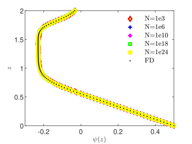
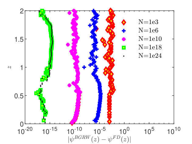
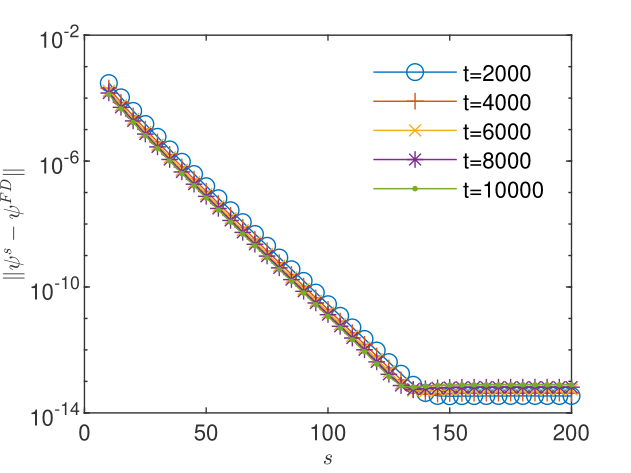
To illustrate the consistency of the representation of the solution by ensembles of random walkers and the equivalence of the BGRW and FD schemes, we compare their solutions for increasing $𝒩$ between ${10}^3$ and ${10}^{24}$ at the final time $T$ (Fig. 2). The errors $|{\psi }^{BGRW}(z)-{\psi }^{FD}(z)|$ of the BGRW solution with respect to the FD solution shown in Fig. 2 decrease as ${𝒩}^{-1}$ and approach the machine precision $\sim {10}^{-16}$ for $𝒩\ge {10}^{18}$. The $l^2$ norm $\Vert {𝝍}^{BGRW}-{𝝍}^{FD}\Vert$ of the difference of the two solution vectors with $I=2/\mathrm{\Delta }z+1=101$ components decreases at a rate of $\sim 10{𝒩}^{-1}$ and reaches a plateau at about ${10}^{-14}$ (see Table 1). Since the FD solution is the ensemble average of the BGRW solution (see Remark 1), this behavior also illustrates the self-averaging property of the GRW algorithms [22].

$𝒩$	1e3	1e6	1e10	1e18	1e24
$\overline{\left|{\psi }^{BGRW}\left(z\right)-{\psi }^{FD}\left(z\right)\right|}$	1.70e-03	4.24e-06	2.52e-10	7.13e-16	9.21e-16
$\Vert {𝝍}^{BGRW}-{𝝍}^{FD}\Vert$	2.27e-02	6.52e-05	3.32e-09	1.13e-14	1.40e-14

Table 1. Mean errors and error norms for Section 3.1, Fig. 2.

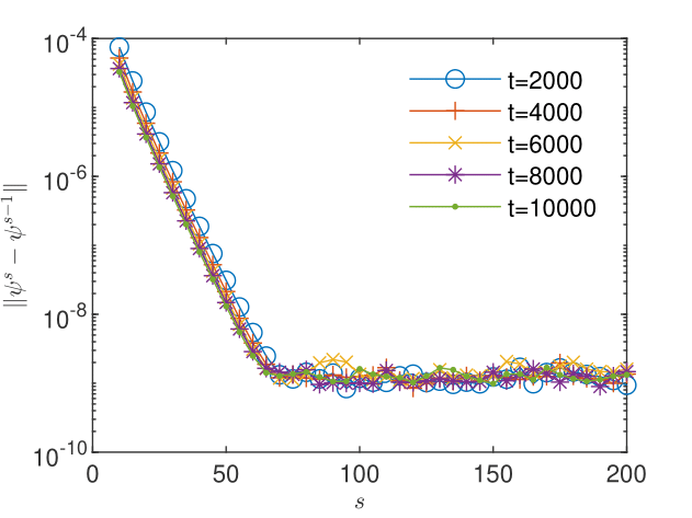
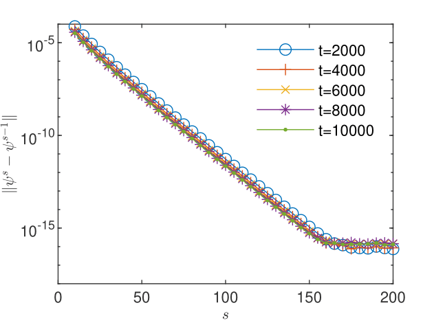
Let $\{{\psi }^s\}$ be the sequence of iterates of the BGRW $L$-scheme and ${𝝍}^{BGRW}=\underset{s\to \mathrm{\infty }}{lim}{𝝍}^s$. By the triangle inequality $\Vert {𝝍}^s-{𝝍}^{s-1}\Vert \le \Vert {𝝍}^s-{𝝍}^{FD}\Vert +\Vert {𝝍}^{FD}-{𝝍}^{s-1}\Vert$ we have $\underset{s\to \mathrm{\infty }}{lim}\Vert {𝝍}^s-{𝝍}^{s-1}\Vert \le 2\Vert {𝝍}^{BGRW}-{𝝍}^{FD}\Vert$. Hence, the order $\sim 20{𝒩}^{-1}$ of convergence of the BGRW solution to the FD solution is an upper limit for corrections. Fig. 4 and Fig. 4 show the decrease of the correction norms for $𝒩={10}^{10}$ and $𝒩={10}^{18}$, respectively. In the first case the corrections reach a plateau of about ${10}^{-9}$, consistent with the upper bound $20{𝒩}^{-1}$. In the second case, the corrections show a plateau at the machine precision, which, as indicated by Fig. 2, is the same as the plateau for the FD scheme.

Remark 7.

The convergence behavior illustrated above can be explained with the reduced fluctuations Algorithm 1. The sum of fractional parts $rest={\sum }_{i=1}^I\{{\delta }_i\}$ can be used to evaluate the truncation errors of the algorithm. At a given lattice site $i$, $\{{\delta }_i\}\in [0,1)$ with a mean $\overline{\{{\delta }_i\}}\approx 0.5$. The sum over the lattice sites is thus $rest\approx 0.5I$. The total numbers of particles on the lattice is $ntot={\sum }_{i=1}^I{n}_{i,k}^s={\sum }_{i=1}^I|{\psi }_{i,k}^s|𝒩=\overline{|\psi |}𝒩I$. With these, the truncation error can be evaluated as $rest/ntot\approx 0.5/\overline{|\psi |}{𝒩}^{-1}$, which is independent of the discretization (i.e., the number of lattice sites $I$). For verification purposes, we remove all the floor functions in the 1, add the truncation sequence

rest=nn+rest; nn=floor(rest); rest=rest-nn;

at the end, and perform the computation with $𝒩={10}^{10}$. The relative error of the solution ${𝛙}_{T/\mathrm{\Delta }t}$ obtained in this way with respect to the solution of the original 1, evaluated with the $l^2$ norm, is of about $4.25\cdot {10}^{-4}$. At the middle of the time interval $[0,T]$ we evaluate $\overline{|\psi |}=6.45\cdot {10}^{-2}$ and obtain the truncation error $0.5/\overline{|\psi |}{𝒩}^{-1}=7.75\cdot {10}^{-10}$, which corresponds to the average value of the plateau shown by the corrections $\Vert {𝛙}^s-{𝛙}^{s-1}\Vert$ in this case. Since the original 1 contains three truncation sequences, we take $rest/I\approx 1.5$ and obtain the truncation error $1.5/\overline{|\psi |}{𝒩}^{-1}=2.30\cdot {10}^{-9}$. This error is almost the same as the plateau of the correction from Fig. 4. The plateau arises when the correction norms reach the threshold given by the truncation errors and cannot be further decreased by the iterative method. We note that this threshold is also close to the relative errors of the BGRW solution with respect to the FD solution at the final time $T$ shown in Fig. 2 and Table 1. Thus, the accuracy of the BGRW $L$-scheme is limited by the truncation errors produced by the reduced fluctuations Algorithm 1.

The plateau of the order $10{𝒩}^{-1}$ also arises if one adds to the three terms depending on the parameter $r$ in the FD 2 a noisy term $randn/𝒩$, where $randn$ is a random variable drawn from the standard normal distribution. The results (not shown here) are similar to those from Fig. 4 and Fig. 6. One expects therefore that the accuracy of the random walk methods based on random number generators is limited as well by truncation errors.

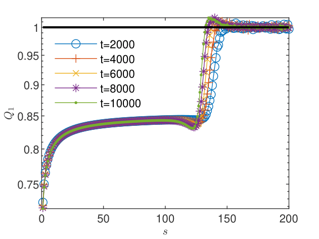
Fig. 6 and Fig. 6 show that the length of the sequence of corrections for $𝒩={10}^{10}$ not affected by oscillations is too short to allow the estimation of the order of convergence $p$ with (29) and the evaluation of the quotient $Q_1$ according to (28). For $𝒩={10}^{18}$, the sequence not affected by oscillations is three times longer and the behavior of the estimate $p(s)\approx 1$ and of the quotient suggest the $C^{\prime }$-linear convergence (see Fig. 8 and Fig. 8). This is, according to Remark 5, a numerical argument for the convergence of the iterates to the unique solution which solves the nonlinear scheme (2.1).

Figure 1. Example 3.1: Comparison of the BGRW (5) and FD (2.1) solutions.

Figure 2. Example 3.1: Errors of the BGRW solutions.

Figure 3. Example 3.1: Corrections ($N={10}^{10}$).

Figure 4. Example 3.1: Corrections ($N={10}^{18}$).

Figure 5. Example 3.1: Estimated order of convergence ($N={10}^{10}$).

Figure 6. Example 3.1: Estimation of the quotient $Q_1$ ($N={10}^{10}$).

Figure 7. Example 3.1: Estimated order of convergence ($N={10}^{18}$).

Figure 8. Example 3.1: Estimation of the quotient $Q_1$ ($N={10}^{18}$).

Figure 9. Example 3.1: Errors of the BGRW solution ($N={10}^{16})$.

Figure 10. Example 3.1: Error-based quotient $Q_1$ of the BGRW solution.

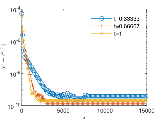
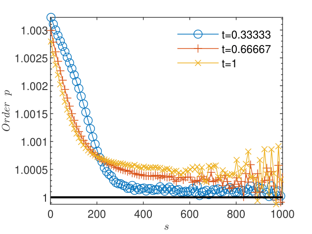
In the absence of an exact solution for this example, we investigate the existence of the “error-based” order $C$ on sequences of errors with respect to the FD solution taken as a reference. We compute BGRW solutions for $𝒩={10}^{16}$ and form the sequence $\{\Vert {𝝍}^s-{𝝍}^{FD}\Vert \}$. The errors presented in Fig. 10 maintain a linear trend in semi-logarithmic representation over 130 iterations $s$ and allow the evaluation, according to (28), of a subunit quotient $Q_1$ in the same interval, shown in Fig. 10. We can therefore assume that the solution of the BGRW scheme converges with the linear $C$-order to the reference FD solution.

3.2. Example 2: fully coupled flow and surfactant transport

The next example is the fully coupled problem of variably saturated flow, with transition from saturated to unsaturated regime, and surfactant transport governed by Eqs. (1) and (2) with the exact manufactured solutions

$${\psi }_m(z,t)=-tz(z-1)+\frac{x}{4},c_m(z,t)=tz(z-1)+1,$$

and the water contend parameterized by

The hydraulic conductivity is constant $K(\theta (\psi ,c))=1$ and the diffusion coefficient in Eq. (2) is set to $D=1$ (in arbitrary units). The manufactured solutions verify Eqs. (1) ans (2) with supplementary source terms [11, 2, 17, 18]. These source terms, generated by inserting the manufactured solutions into the equations, are calculated analytically with the Matlab symbolic toolbox.

We first solve the problem in the domain $[0,1]$, on a regular lattice with $\delta z=2.5\cdot {10}^{-2}$, with the coupled FD scheme (2.1) and BGRW transport scheme (13). The time step $\mathrm{\Delta }t=1.56\cdot {10}^{-3}$ is determined according to (26) with $L_{\psi }=L_c=100$, $\alpha =1$, and $\beta =0.5$. The corrections are evaluated in the $l^2$ norm with the absolute tolerance ${\epsilon }_a={10}^{-18}$ and the convergence is assessed with the condition $\max (\Vert {𝝍}^s-{𝝍}^{s-1}\Vert ,\Vert {𝒄}^s-{𝒄}^{s-1}\Vert )\le {\epsilon }_a$.

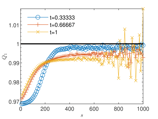
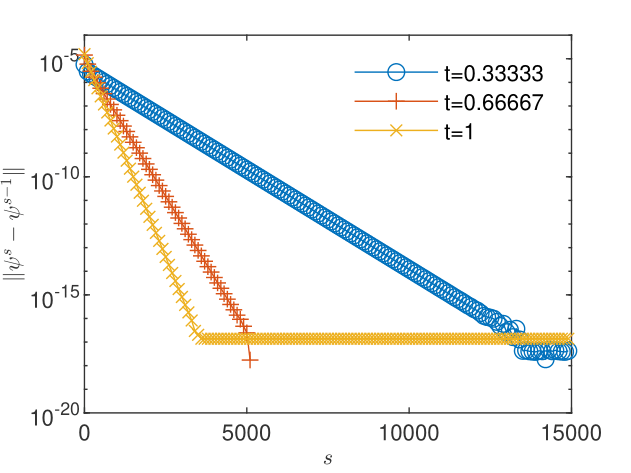
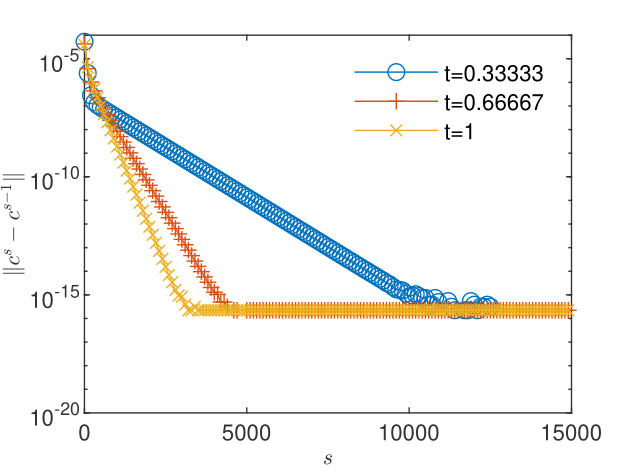
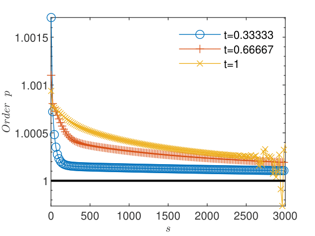
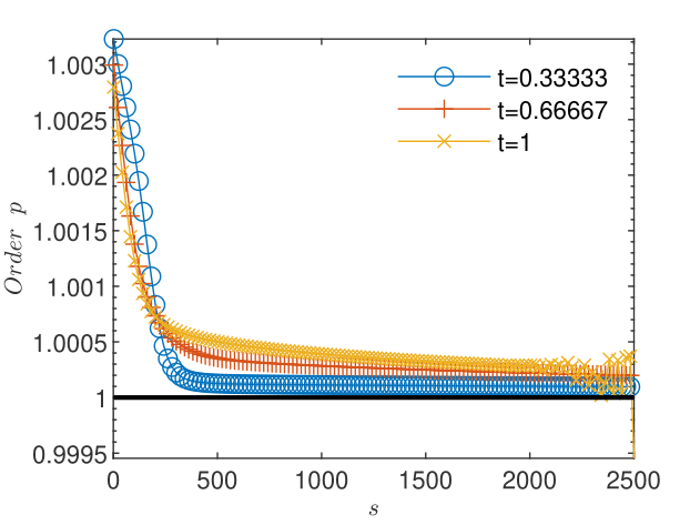
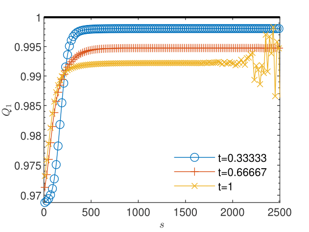
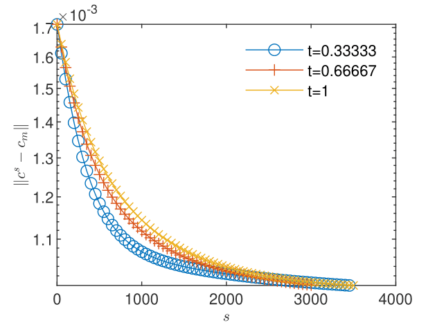
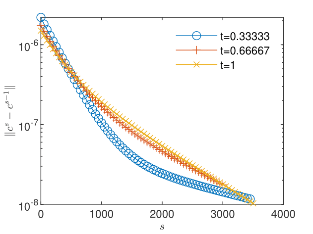
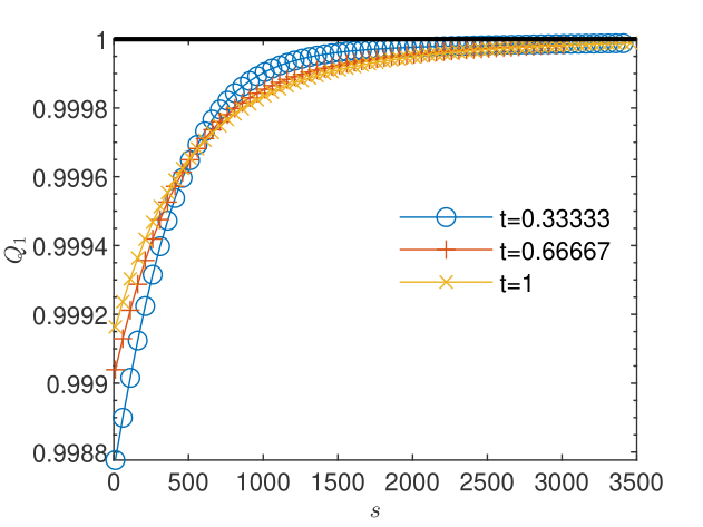
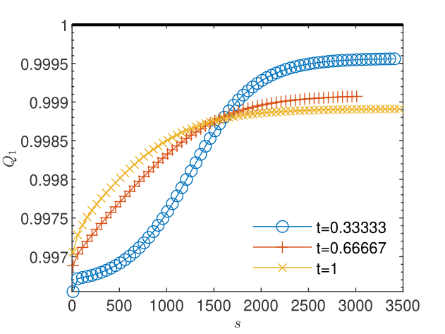
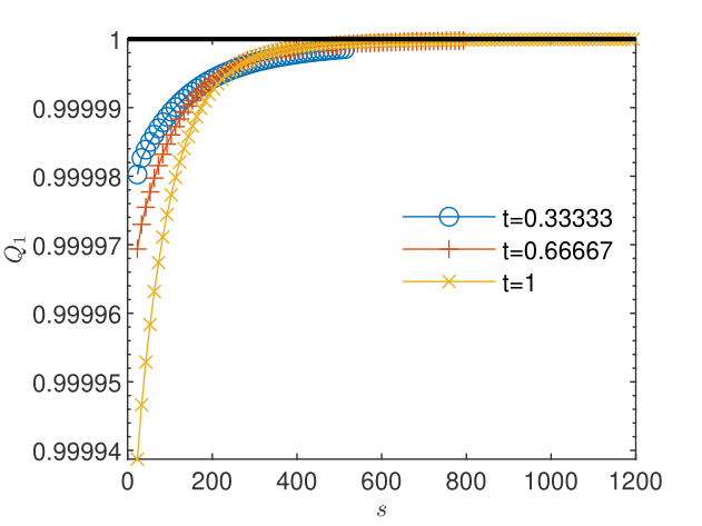
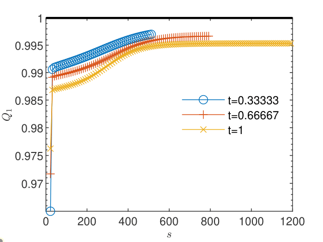
The results obtained for $𝒩={10}^{10}$ particles used in the transport scheme presented in Figs. 12 and 12 show that the truncation errors generated by the transport 3 yield a plateau $\sim {10}^{-10}$ of the concentration corrections and also, due to the coupling, a plateau higher than the machine precision of about ${10}^{-13}$ of the pressure corrections. The oscillations arising when the corrections reach the plateau do not allow reliable estimations of the order of convergence and of the trend of the quotient $Q_1$, for both pressure (Figs. 14 and 14) and concentration (Figs. 16 and 16). Increasing the number of particles in the transport scheme to $𝒩={10}^{24}$ lowers the plateau to the machine precision for both pressure and concentration corrections (Figs. 18 and 18), renders more reliable the estimates of the order of convergence $p=1$ (Figs. 20 and 22), and indicates limits , consistent with the $C^{\prime }$ linear convergence (Figs. 20 and 22). According to Remark 5, this result is an indication of the convergence to the solution of the nonlinear schemes (2.1) and (2.2).

Tests (not presented here) with a similar two dimensional problem [17, Sec. 5.2.1] also show the plateau $\sim {10}^{-13}$ of the pressure corrections produced by the coupling of flow and transport for $𝒩={10}^{10}$ particles in the transport code and a plateau at the machine precision for $𝒩={10}^{24}$ particles.

Figure 11. Example 3.2: Corrections, of the pressure solution ($N={10}^{10}$).

Figure 12. Example 3.2: Corrections of the concentration solution ($N={10}^{10}$).

Figure 13. Example 3.2: Estimation of the convergence order $p$, pressure ($N={10}^{10}$).

Figure 14. Example 3.2: Estimation of the quotient $Q_1$, pressure ($N={10}^{10}$).

Figure 15. Example 3.2: Estimation of the convergence order $p$, concentration ($N={10}^{10}$).

Figure 16. Example 3.2: Estimation of the quotient $Q_1$, concentration ($N={10}^{10}$).

Figure 17. Example 3.2: Corrections of the pressure solution ($N={10}^{24}$).

Figure 18. Example 3.2: Corrections of the concentration solution ($N={10}^{24}$).

Figure 19. Example 3.2: Estimation of the convergence order $p$, pressure ($N={10}^{24}$).

Figure 20. Example 3.2: Estimation of the quotient $Q_1$, pressure ($N={10}^{24}$).

Figure 21. Example 3.2: Estimation of the convergence order $p$, concentration ($N={10}^{24}$).

Figure 22. Example 3.2: Estimation of the quotient $Q_1$, concentration ($N={10}^{24}$).

The convergence of the iterations does not yet ensure the convergence of the numerical solution to the manufactured solution. This can be verified by a grid convergence test performed by successively halving the space step $\mathrm{\Delta }z$. To do that, we fix the number of particles in the transport code to $𝒩={10}^{24}$, which, as seen above, ensures that the truncation errors do not affect the convergence of the corrections, and perform iterations of the linearization schemes (2.1) and (13) until the corrections fall below the threshold ${\epsilon }_a={10}^{-18}$. The solutions for successive $\mathrm{\Delta }z$ are further used to evaluate the EOC by the rate of logarithmic decay of the deviations from the manufactured solutions measured with the discrete $L^2$ norm $\sqrt{\mathrm{\Delta }z}\parallel \cdot {\parallel }_{l^2}$. The results presented in Table 2 indicate the second order convergence of the solution $\{𝝍,𝒒,𝒄\}$.

$\mathrm{\Delta }z$	$\Vert \psi -{\psi }_m\Vert$	EOC	$\Vert q-m_m\Vert$	EOC	$\Vert c-c_m\Vert$	EOC
1.00e-1	4.59e-02	–	1.23e-01	–	3.43e-02	–
5.00e-1	1.14e-02	2.01	3.34e-02	1.89	1.02e-02	1.75
2.50e-2	2.85e-03	2.00	8.68e-03	1.94	2.76e-03	1.88
1.25e-2	7.11e-04	2.00	2.21e-03	1.98	7.21e-04	1.94

Table 2. Orders of convergence of the numerical solution to Example 3.2.

The knowledge of the exact solution allows us to compute error-based orders of convergence as well. Using a finer discretization, $\mathrm{\Delta }z=1.25\cdot {10}^{-2}$, and a larger tolerance ${\epsilon }_a={10}^{-3}$ we form sequences of discrete $L^2$ norms of errors and corrections for pressure (Figs. 24 and 24) and concentration (Figs. 26 and 26). We note that as the convergence criterion for errors is fulfilled, the corrections are four to five orders of convergence smaller. Estimations (not shown here) of the order of convergence $p$ with (29) were found to be consistent with the definition of the $Q$ linear convergence, for both errors and the corresponding corrections. The quotient $Q_1$ computed with (28) from the sequences of successive errors approaches the unity, indicating the $C$ sublinear convergence of the linearization schemes for both flow and transport (Figs. 28 and 30). We have thus an illustration of the observation made in Remark 6 that $C$-linear convergence cannot be obtained in numerical simulations. For the corresponding corrections, indicates the $C^{\prime }$-linear convergence (Figs. 28 and 30), which, according to Remark 5, indicates the convergence of the iterative schemes to the solutions of the coupled nonlinear schemes (2.1) and (2.2).

Figure 23. Example 3.2: Errors of the pressure solution.

Figure 24. Example 3.2: Corrections of the pressure solution.

Figure 25. Example 3.2: Errors of the concentration solution.

Figure 26. Example 3.2: Corrections of the concentration solution.

Figure 27. Example 3.2: Estimation of the quotient $Q_1$, pressure errors.

Figure 28. Example 3.2: Estimation of the quotient $Q_1$, pressure corrections.

Figure 29. Example 3.2: Estimation of the quotient $Q_1$, concentration errors.

Figure 30. Example 3.2: Estimation of the quotient $Q_1$, concentration corrections.

3.3. Example 3: One-way coupled flow and transport problem with van Genuchten-Mualem parameterization

In the following, we consider the one-way coupled system (1)-(2), i.e., $\theta$ independent of $c$, with an experimentally based parameterization model. The relationships defining the water content $\theta (\psi )$ and the hydraulic conductivity $K(\theta (\psi ))$ are given by the van Genuchten-Mualem model

(35)

(36)

where $\mathrm{\Theta }=(\theta -{\theta }_{res})/({\theta }_{sat}-{\theta }_{res})$ is the normalized water content defined in the same way as for the exponential model (33)-(34), $\alpha$, $n$, $m=1-1/n$ are model parameters depending on the soil type, and $K_{sat}$ is the constant hydraulic conductivity in the saturated regime. In this example, we consider the parameters of a silt loam used in previously published studies [8, 17, 18], ${\theta }_{sat}=0.396$, ${\theta }_{res}=0.131$, $\alpha =0.423$, $n=2.06$, $K_{sat}=4.96\cdot {10}^{-2}$.

We chose the manufactured solutions

$${\psi }_m(z,t)=-tz(z-1)-\frac{x}{4}+\frac{x}{2},c_m(z,t)=tz(z-1)+1,$$

which illustrate again the degeneracy of Richards’ equation, with transitions from saturated to unsaturated flow regime. The diffusion coefficient in the transport equation (2) is set to $D=0.01$. The source terms generated by the manufactured solutions are calculated as in Section 3.2 above with the Matlab symbolic toolbox.

Since the flow is now independent of transport it is not influenced the truncation produced by the 3. Therefore, we focus here on the error-based orders of convergence of the linearization schemes. The coupled problems are solved in the domain $[0,1]$, with $\mathrm{\Delta }z=1.25\cdot {10}^{-2}$ and $\mathrm{\Delta }t=3.91\cdot {10}^{-3}$. The convergence is assessed with discrete $L^2$ norms of pressure and concentration errors with respect to the manufactured solutions for the tolerance ${\epsilon }_a={10}^{-3}$. Preliminary tests with increasing numbers of particles show that the transport scheme (13) fails to converge if . To completely eliminate the effect to the truncation errors, the computations are carried out with $𝒩={10}^{18}$ particles.

As in the previous example, we found that the correction norms reach values that are systematically smaller by several orders of magnitude than the error norms, for both pressure and concentration and the estimates obtained with (29) indicate the $Q$ order of convergence $p=1$. The quotient $Q_1$ computed with (28) approaches the unity for the errors of both the pressure and the concentration (Figs. 32 and 34) indicating the sublinear convergence. For the corresponding corrections (Figs. 32 and 34) , hence the $C^{\prime }$ linear convergence of both iterative schemes may be assumed. These results illustrate again the observations made in Remarks 5 and 6.

Figure 31. Example 3.3: Estimation of the quotient $Q_1$, pressure errors.

Figure 32. Example 3.3: Estimation of the quotient $Q_1$, pressure corrections.

Figure 33. Example 3.3: Estimation of the quotient $Q_1$, concentration errors.

Figure 34. Example 3.3: Estimation of the quotient $Q_1$, concentration corrections.

The grid convergence test, conducted in the same way as in Section 3.2, presented in Table 3 indicates the quadratic convergence of the solution $\{𝝍,𝒒,𝒄\}$ towards the exact manufactured solution.

$\mathrm{\Delta }z$	$\Vert \psi -{\psi }_m\Vert$	EOC	$\Vert q-m_m\Vert$	EOC	$\Vert c-c_m\Vert$	EOC
1.00e-1	5.85e-02	–	2.28e-03	–	1.23e-02	–
5.00e-1	1.42e-02	2.05	5.69e-04	2.00	3.54e-03	1.80
2.50e-2	3.27e-03	2.11	1.48e-04	1.94	9.19e-04	1.95
1.25e-2	8.09e-04	2.02	4.50e-05	1.72	2.38e-04	1.95

Table 3. Orders of convergence of the numerical solution to Example 3.3.

4. Conclusions

In this study, we demonstrated through numerical examples the convergence of the explicit $L$-schemes for nonlinear and degenerate problems of coupled flow and transport processes in porous media. The convergence issue is two-fold. First it is the convergence of the iterative method which solves the nonlinearity of the problem and provides a solution of the nonlinear numerical scheme, for instance the $L$-scheme for Richards’ equation (2.1) which approximates the solution of the nonlinear scheme (2.1). The second aspect is the convergence of the numerical solution to the exact solution of the problem, provided that there exists a unique solution.

The convergence of the iterative schemes has been investigated through estimations of computational and error-based orders of convergence. The three examples presented in Section 3 provide numerical arguments for the $C^{\prime }$-linear convergence. According to Remark 5, the $C^{\prime }$-linear convergence indicates the uniqueness of the iterative solutions and their convergence to the solutions of the nonlinear schemes. The sequences of errors with respect to exact manufactured solutions of the coupled problem presented in Section 3.2 and Section 3.3 are only sublinearly $C$ convergent and illustrate the impossibility of achieving the $C$-liner convergence via numerical simulations, pointed out in Remark 6. However, with the FD solution as reference, we have shown that the random walk BGRW $L$-scheme for Richards’ equation could be $C$-linear convergent (Fig. 10). Using grid convergence tests and manufactured solutions we get strong numerical evidence of second order convergence ($\sim {(\mathrm{\Delta }z)}^2$) of the $L$-schemes for coupled flow and transport problems (Table 2 and Table 3).

The random walk method for Richards’ equation is rather of academic interest. It has been used, for instance, to prove the stability of the equivalent FD scheme (Remark 1). Instead, the random walk approach is essential in modeling the transport because it facilitates a discrete description at the molecular level of the chemical reactions [18] and provides a basis for the space-time upscaling of the reactive transport in porous media [19]. An issue of concern of this approach are the truncation errors produced by the Algorithm 1 which preserves the indivisibility of the particles. We have shown that the truncation errors induce a plateau in the decrease of the successive corrections of the linearization method (Remark 7). The plateau is inversely proportional to the number of particles, $\sim {𝒩}^{-1}$, and may hinder the evaluation of the convergence orders if $𝒩$ is not large enough. In modeling reactive transport, where the amount of molecules is of the order of Avogadro’s number, the plateau reaches the machine precision. However, the truncation-limited precision becomes significant in applications for small systems of particles (e.g., [21]), for instance in modeling the isotopic separation of heavy water where the number of deuterium isotopes can be of the order $𝒩\sim {10}^6$ or even smaller.

Acknowledgements.

F.A. Radu acknowledges the support of the VISTA program, The Norwegian Academy of Science and Letters, and Equinor.

References

- [1]
- [2] C.D. Alecsa, I. Boros, F. Frank, P. Knabner, M. Nechita, A. Prechtel, A. Rupp and N. Suciu, Numerical benchmark study for fow in heterogeneous aquifers, Adv. Water Resour., 138 (2020), 103558. https://doi.org/10.1016/j.advwatres.2020.103558
- [3] E. Cătinaş, A survey on the high convergence orders and computational convergence orders of sequences, Appl. Math. Comput. 343 (2019), pp. 1–20. https://doi.org/10.1016/j.amc.2018.08.006
- [4] E. Cătinaş, How many steps still left to x*?, SIAM Rev. 63 (2021) no. 3, pp. 585–624. https://doi.org/10.1137/19M1244858
- [5] D. Illiano, I.S. Pop and F.A. Radu, Iterative schemes for surfactant transport in porous media, Comput. Geosci. 25 (2021), 805–822. https://doi.org/10.1007/s10596-020-09949-2
- [6] P. Knabner, S. Bitterlich, R. Iza Teran, R., A. Prechtel and E. Schneid, Influence of surfactants on spreading of contaminants and soil remediation, pp.152-161 In: Jäger, W., Krebs, H.J. (Eds.), Mathematics –Key Technology for the Future, Springer, Berlin, Heidelberg, 2003. https://doi.org/10.1007/978-3-642-55753-8_12
- [7] P. Knabner and L. Angermann, Numerical Methods for Elliptic and Parabolic Partial Differential Equations. Springer, New York, 2003. https://doi.org/10.1007/b97419
- [8] F. List and F.A. Radu, A study on iterative methods for solving Richards’ equation, Comput. Geosci. 20 (2016) no. (2), 341–353. https://doi.org/10.1007/s10596-016-9566-3
- [9] I.S. Pop, F.A. Radu and P. Knabner, Mixed finite elements for the Richards’ equation: linearization procedure, J. Comput. Appl. Math. 168 (2004) no. 1, pp. 365–373 https://doi.org/10.1016/j.cam.2003.04.008
- [10] F.A. Radu, K. Kumar, J.M. Nordbotten and I.S. Pop, A robust, mass conservative scheme for two-phase flow in porous media including Hölder continuous nonlinearities, IMA Journal of Numerical Analysis, 38 (2018) no. 2, pp.884–920. urlhttps://doi.org/10.1093/imanum/drx032
- [11] P.J. Roache, Code verification by the method of manufactured solutions, J. Fluids Eng. 124 (2002) no. 1, pp. 4–10. http://dx.doi.org/10.1115/1.1436090
- [12] C.J. Roy, Review of code and solution verification procedures for compu- tational simulation, J. Comput. Phys. 205 (2005), 131–156. https://doi.org/10.1016/j.jcp.2004.10.036
- [13] J.S. Stokke, K. Mitra, E. Storvik, J.W. Both and F.A. Radu, An adaptive solution strategy for Richards’ equation, Comput. Math. Appl. 152 (2023), 155–167. https://doi.org/10.1016/j.camwa.2023.10.020
- [14] J.C. Strikwerda, Finite Difference Schemes and Partial Differential Equations, SIAM, 2004. https://doi.org/10.1137/1.9780898717938
- [15] N. Suciu, Diffusion in Random Fields. Applications to Transport in Groundwater, Birkhäuser, Cham, 2019. https://doi.org/10.1007/978-3-030-15081-5
- [16] N. Suciu, Global Random Walk Solutions for Flow and Transport in Porous Media, in F.J. Vermolen and C. Vuik (eds.), Numerical Mathematics and Advanced Applications ENUMATH 2019, Lecture Notes in Computational Science and Engineering 139, Springer Nature, Switzerland, 2020. https://doi.org/10.1007/978-3-030-55874-1_93
- [17] N. Suciu, D. Illiano, A. Prechtel and F.A. Radu, Global random walk solvers for fully coupled flow and transport in saturated/unsaturated porous media, Adv. Water Resour. 152 (2021), 103935. https://doi.org/10.1016/j.advwatres.2021.103935
- [18] N. Suciu and F.A. Radu, Global random walk solvers for reactive transport and biodegradation processes in heterogeneous porous media, Adv. Water Res., 166 (2022), 104268. https://doi.org/10.1016/j.advwatres.2022.104268
- [19] N. Suciu, F.A. Radu and I.S. Pop, Space-time upscaling of reactive transport in porous media, Adv. Water Resour. 176 (2023), 104443. http://dx.doi.org/10.1016/j.advwatres.2023.104443
- [20] N. Suciu, F.A. Radu, J.S. Stokke, E. Cătinaş and A. Malina, Computational orders of convergence of iterative methods for Richards’ equation, arXiv preprint arXiv:2402.00194 (2024), https://doi.org/10.48550/arXiv.2402.00194
- [21] C. Vamoş, N. Suciu and M Peculea, Numerical modelling of the one-dimensional diffusion by random walkers, Rev. Anal. Numér. Théor. Approx., 26 (1997) no. 1-2, pp. 237–247. https://ictp.acad.ro/jnaat/journal/article/view/1997-vol26-nos1-2-art32/
- [22] C. Vamoş, N. Suciu and H. Vereecken, Generalized random walk algorithm for the numerical modeling of complex diffusion processes, J. Comput. Phys., 186 (2003), pp. 527–544. https://doi.org/10.1016/S0021-9991(03)00073-1