Return to Article Details Convergence of the θ-Euler-Maruyama method for a class of stochastic Volterra integro-diﬀerential equations

Convergence of the $\theta$ -Euler-Maruyama method for a class of Stochastic Volterra Integro-Differential Equations

Samiha Mouchir^∗ and Abdeldjalil Slama^∗

(Date: May 29, 2024; accepted: November 14, 2024; published online: December 18, 2024.)

Abstract.

This paper addresses the convergence analysis of the $\theta$ -Euler-Maruyama method for a class of stochastic Volterra integro-differential equations (SVIDEs). At first, we discuss the existence, uniqueness, boundedness and Hölder continuity of the theoretical solution. Subsequently, the strong convergence order of the $\theta$ -Euler-Maruyama approach for SVIDEs is established. Finally, we provided numerical examples to illustrate the theoretical results.

Key words and phrases:

Stochastic Volterra integro-differential equations,

\Theta

-Euler-Maruyama method, strong convergence, Hölder continuity.

2005 Mathematics Subject Classification:

65C30, 60B10, 65L20.

^∗Laboratory of Mathematics, Modeling and Applications (LaMMA), University of Adrar, Adrar, Algeria. mou.samiha @univ-adrar.edu.dz, aslama@univ-adrar.edu.dz

1. Introduction

Stochastic differential equations (SDEs) have attracted significant attention and are currently emerging as a modeling tool in various scientific fields, including but not limited to telecommunications (see [15]), economics, finance (see [5]), biology, chemistry, and quantum field theory.

The Volterra integral equations (VIEs) were proposed by Vito Volterra, which Traian Lalescu later studied in his 1908 thesis ”Sur les équations de Volterra”, written under the direction of Émile Picard. Volterra integral equations find application in viscoelastic materials, fluid mechanics, and demography (see, e.g., [10],[3], [17],[8],[7]). Stochastic Volterra integral equations (SVIEs) are an extension of ordinary Volterra integral equations to include random noise, making them suitable for modeling systems with stochastic components. SVIEs find applications in various fields, including mathematical finance, biology, physics and engineering. For example, in finance, SVIEs are used to model the evolution of financial asset prices over time, taking into account the stochastic nature of market movements. In biology, they can be used to describe population dynamics subject to random environmental factors. Therefore, in recent years, SVIEs have attracted the attention of many researchers. For instance (see [10],[17],[8],[7]). The exact methods for solving stochastic differential equations (SDEs) involve addressing current challenges in the field (cf. [6], [16], [3], [11], [4], [17], [13], [7]). While there are many analytical methods available, the complexity of these equations makes it difficult to obtain exact solutions. Among the numerical methods are the Milstein method, Runge-Kutta method see [1], Euler-Maruyama method, stochastic theta method, and others (see [10], [9],[12],[2], [17]). Zong et al. [18] conducted a study on two classes of theta-Milstein schemes for stochastic differential equations in terms of convergence and stability.

Recently, Deng et al. [4] examined the semi-implicit Euler method for non-linear time changed stochastic diferential equations. Wang et al. [14] investigated the stochastic theta methods (STMs) for stochastic differential equations (SDEs) with non-global Lipschitz drift and diffusion coefficients. Zhang et al. [17] examined the Euler-Maruyama (EM) method’s numerical analysis of the following generalized SVIDEs:

	$\displaystyle dY(t)=$	$\displaystyle f\bigg{(}Y(t),\int_{0}^{t}K_{1}(t,s)Y(s)ds,\int_{0}^{t}\sigma_{1%}(t,s)Y(s)dB(s)\bigg{)}dt$
		$\displaystyle+g\bigg{(}Y(t),\int_{0}^{t}K_{2}(t,s)Y(s)ds,\int_{0}^{t}\sigma_{2%}(t,s)Y(s)dB(s)\bigg{)}dB(t).$

Lan et al. [7] presented the $\theta$ -EM method corresponding to the following SVIDEs:

dX(t)=f\bigg{(}X(t),\int_{0}^{t}G(t-s)X(s)ds\bigg{)}dt+g\bigg{(}X(t),\int_{0}^%{t}H(t-s)X(s)ds\bigg{)}dB(t).

Inspired and motivated by the above works [4, 14, 17, 7], in this paper, we study the strong convergence of the $\theta$ -Euler-Maruyama method for a class of stochastic Volterra integro-differential equations (SVIDEs) as follows:

(1.1)

dY(t)=f\bigg{(}Y(t),\int_{0}^{t}\sigma_{1}(t,s)Y(s)dB(s)\bigg{)}dt+g\bigg{(}Y(%t),\int_{0}^{t}\sigma_{2}(t,s)Y(s)ds\bigg{)}dB(t),\hskip 5.69046ptt\in[0,T],

with initial condition $Y(0)=Y_{0}\in\mathbb{R}$ , where $f:\mathbb{R}\times\mathbb{R}\rightarrow\mathbb{R}$ and $g:\mathbb{R}\times\mathbb{R}\rightarrow\mathbb{R}$ are given functions. The kernels $\sigma_{i}:D\rightarrow\mathbb{R}$ are continuous on $D:=\left\{(t,s):0\leq s\leq t\leq T\right\}$ with the norm $\lVert\sigma_{i}\rVert_{\infty}=\max_{(t,s)\in D}|\sigma_{i}(t,s)|$ for $i=1,2$ . $Y(t)$ is a stochastic processes defined on probability space $(\Omega,\mathcal{F},\mathbb{P})$ , $B(t)$ is a standard Brownian motion (1-dimensional Brownian motion) defined on the same probability space. And $\mathbb{E}\lVert Y_{0}\rVert^{2}<\infty$ .

The structure of this paper is as follows: We introduce some fundamental notations and preliminaries in Section 2. We then present the definition of the solution of equation (1.1) and investigate the existence, uniqueness, boundedness and Hölder continuity of the analytic solution in Section 3. The $\theta$ -EM method for equation (1.1) is presented, and its order of convergence is taken into account in Section 4. Finally, we provide numerical examples in Section 5 to illustrate the theoretical results.

2. Preliminaries

Let $(\Omega,\mathcal{F},(\mathcal{F}_{t})_{t\geq 0},\mathbb{P})$ be a complete probability space with a filtration $(\mathcal{F}_{t})_{t\geq 0}$ satisfying the usual conditions , and let $\mathbb{E}$ denote the expectation corresponding to $\mathbb{P}$ . A 1-dimensional Brownian motion defined on the probability space is denoted by $B(t)$ . Let $L^{2}([0,T],\mathbb{R})$ by the family of Borel measurable functions $\Phi:[0,T]\rightarrow\mathbb{R}$ such that for every $T>0,\hskip 5.69046pt\int_{0}^{T}|\Phi(t)|^{2}dt<\infty.$ We denote $\mathcal{L}^{2}(\left[0,T\right],\mathbb{R})$ the family of $\mathbb{R}$ -valued $\mathcal{F}_{t}$ -adapted processes $\{\Phi(t)\}_{t\in\left[0,T\right]}$ such that $\int_{0}^{T}|\Phi(t)|^{2}dt<\infty.$ $\mathcal{M}^{2}(\left[0,T\right],\mathbb{R})$ be the family of processes $\mathcal{F}_{t}-$ adapted $\{\Phi(t)\}_{t\in\left[0,T\right]}\in\mathcal{L}^{2}(\left[0,T\right],\mathbb{%R})$ such that $\mathbb{E}\left[\int_{0}^{T}|\Phi(t)|^{2}dt\right]<\infty$ . For $a,b\in\mathbb{R},\,a\wedge b:=\min\left\{a,b\right\},\,\text{and}\,a\vee b:=%\max\left\{a,b\right\}$ . If $\mathbb{D}$ is a subset of $\Omega$ , the indicator function is denoted by $1_{\mathbb{D}}$ . We can write the integral of equation (1.1) as follows:

	$\displaystyle Y(t)$	$\displaystyle=Y(0)+\int_{0}^{t}f\bigg{(}Y(u),\int_{0}^{u}\sigma_{1}(u,s)Y(s)dB%(s)\bigg{)}du$
(2.2)			$\displaystyle\quad+\int_{0}^{t}g\bigg{(}Y(u),\int_{0}^{u}\sigma_{2}(u,s)Y(s)ds%\bigg{)}dB(u).$

We will introduce the definition of the solution, we assume that $Y(.)\in\mathcal{L}^{2}(\left[0,T\right],\mathbb{R})$ where

	$\displaystyle F(t):=$	$\displaystyle f\bigg{(}Y(t),\int_{0}^{t}\sigma_{1}(t,s)Y(s)dB(s)\bigg{)},$
	$\displaystyle G(t):=$	$\displaystyle g\bigg{(}Y(t),\int_{0}^{t}\sigma_{2}(t,s)Y(s)ds\bigg{)}.$

Definition 2.1.

A solution of (2) is a continuous stochastic process $\{Y(t)\}_{t\in\left[0,T\right]}$ with values in $\mathbb{R}$ satisfies the following conditions:

i)

$Y(.)\in\mathcal{L}^{2}(\left[0,T\right],\mathbb{R}),\hskip 5.69046ptF(.)\in%\mathcal{L}^{1}(\left[0,T\right],\mathbb{R})$ and $G(.)\in\mathcal{L}^{2}(\left[0,T\right],\mathbb{R})$ ,
ii)

(2) holds for all $t\in\left[0,T\right]$ with probability 1. The solution $\{Y(t)\}$ is said to be unique if there is exists other solution $\{\overline{Y}(t)\}$ such that $\{Y(t)\}=\{\overline{Y}(t)\}$ for all $t\in\left[0,T\right]$ , i.e.,

$\mathbb{P}\Big{\{}Y(t)=\overline{Y}(t)\hskip 5.69046pt\text{for all}\hskip 5.6%9046ptt\in\left[0,T\right]\Big{\}}=1.$

Definition 2.2.

Let $0<\delta\leq 1$ . A stochastic process $Y(t,\omega):\left[0,T\right]\times\Omega\rightarrow\mathbb{R}$ is referred to as Hölder continuous with exponent $\delta>0$ if a constant M exists such that

\mathbb{E}|Y(t)-Y(r)|^{2}\leq M|t-r|^{2\delta},\hskip 14.22636pt\forall t,r\in%\left[0,T\right].

In this article, we propose the following hypotheses.

(1)

( $H_{1}$ ) (Lipschiz condition). Assume that there exist a positive constant $K$ such that

$\Big{|}f(x,y)-f(x^{\prime},y^{\prime})\Big{|}^{2}\vee\Big{|}g(x,y)-g(x^{\prime%},y^{\prime})\Big{|}^{2}\leq K\Big{(}\big{|}x-x^{\prime}\big{|}^{2}+\big{|}y-y%^{\prime}\big{|}^{2}\Big{)},$

for $x,y,x^{\prime},y^{\prime}\in\mathbb{R}$ .
(2)

( $H_{2}$ ) (Linear growth condition). For $x,y\in\mathbb{R}$

$\big{|}f(x,y)\big{|}^{2}\vee\big{|}g(x,y)\big{|}^{2}\leq K^{\prime}\Big{(}1+%\big{|}x\big{|}^{2}+\big{|}y\big{|}^{2}\Big{)},$

where $K^{\prime}=2\Big{(}K\vee|f(0,0)|^{2}\vee|g(0,0)|^{2}\Big{)}$ .
(3)

( $H_{3}$ ) (Mean value theorem). Assuming that the coefficients $\sigma_{i}\in C^{1}(D),$ for $i=1,2.$ of (1.1) satisfy

$\big{|}\sigma_{i}^{\prime}(t,s)\big{|}^{2}\leq K^{\prime\prime},$

with $K^{\prime\prime}>0,$ for all $(t,s)\in D,$ and

$\Big{|}\sigma_{i}(u,s)-\sigma_{i}(u_{h},s)\Big{|}^{2}=\Big{|}\sigma_{i}(\xi_{i%},s)(u,u_{h})\Big{|}^{2}\leq K^{\prime\prime}h^{2},$

where $\xi_{i}\in(u,u_{h})$ .

The existence and uniqueness of the solution to (1.1) under hypothesis ( $H_{2}$ ) are demonstrated by the following theorem. The proof of this theorem is similar to the proof in [17], which pertains to the case where $\Theta=0.$

3. Theoretical analysis of the class of SVIDE

In this section, we present the theoretical results. The existence and uniqueness of the solution to (2) have been established. Additionally, we verified the Hölder continuity condition for the analytical solutions.

3.1. The existence and uniqueness of the analytical solution

We now discuss the theory of existence and uniqueness of the solution of the equation (2). We first present the following lemma.

Lemma 3.1.

Assume that ( $H_{2}$ ) is satisfied. If $Y(t)\in\mathcal{L}^{2}(\left[0,T\right],\mathbb{R})$ is a solution of SVIDEs (1.1), and such that

(3.3)

\mathbb{E}\left[Y(t)\right]^{2}\leq M_{0},\hskip 14.22636pt\forall t\in\left[0%,T\right],

where $M_{0}$ depends on $\sigma_{1},\sigma_{2},T,K^{\prime}$ and $Y_{0}$ .

Proof.

For every integer $n\geq 1,\,\tau_{n}$ be a stopping time such that

\tau_{n}=T\wedge\inf\Big{\{}t\in\left[0,T\right]:|Y(t)|\geq n\Big{\}}.

Evidently, $\tau_{n}\rightarrow T$ a.s. by letting $n\rightarrow\infty.$ Define $Y_{n}(t):=Y(t\wedge\tau_{n})$ for $t\in\left[0,T\right]$ . It can be verified that $Y_{n}(t)$ satisfies.

	$\displaystyle Y_{n}(t)$	$\displaystyle=Y(0)+\displaystyle\int_{0}^{t}f\bigg{(}Y_{n}(u),\displaystyle%\int_{0}^{u}\sigma_{1}(u,s)Y_{n}(s)\mathbf{1}_{\left[0,\tau_{n}\right]}(s)dB(s%)\bigg{)}\mathbf{1}_{\left[0,\tau_{n}\right]}(u)du$
		$\displaystyle\quad+\displaystyle\int_{0}^{t}g\bigg{(}Y_{n}(u),\displaystyle%\int_{0}^{u}\sigma_{2}(u,s)Y_{n}(s)\mathbf{1}_{\left[0,\tau_{n}\right]}(s)ds%\bigg{)}\mathbf{1}_{\left[0,\tau_{n}\right]}(u)dB(u),\hskip 14.22636ptt\in%\left[0,T\right].$

By Cauchy’s inequality, the Itô isometry, and the inequality $(x+y+z)^{2}\leq 3(x^{2}+y^{2}+z^{2})$ , we obtain that

	$\displaystyle\|Y_{n}(t)\|^{2}$	$\displaystyle\leq 3\|Y_{0}\|^{2}+3t\displaystyle\int_{0}^{t}\bigg{\|}f\bigg{(}Y_{%n}(u),\displaystyle\int_{0}^{u}\sigma_{1}(u,s)Y_{n}(s)\mathbf{1}_{\left[0,\tau%_{n}\right]}(s)dB(s)\bigg{)}\mathbf{1}_{\left[0,\tau_{n}\right]}(u)\bigg{\|}^{2%}du$
		$\displaystyle\quad+3\displaystyle\int_{0}^{t}\bigg{\|}g\bigg{(}Y_{n}(u),%\displaystyle\int_{0}^{u}\sigma_{2}(u,s)Y_{n}(s)\mathbf{1}_{\left[0,\tau_{n}%\right]}(s)ds,\bigg{)}\mathbf{1}_{\left[0,\tau_{n}\right]}(u)\bigg{\|}^{2}du.$

Using Cauchy’s inequality and the Itô isometry, we show that

(3.4)

\mathbb{E}|Y_{n}(t)|^{2}\leq 3\mathbb{E}|Y_{0}|+3TF+3G,

where

F:=\mathbb{E}\bigg{[}\int_{0}^{t}\bigg{|}f\bigg{(}Y_{n}(u),\int_{0}^{u}\sigma_%{1}(u,s)Y_{n}(s)\mathbf{1}_{\left[0,\tau_{n}\right]}(s)dB(s)\bigg{)}\mathbf{1}%_{\left[0,\tau_{n}\right]}(u)\bigg{|}^{2}du\bigg{]},

and

G:=\mathbb{E}\bigg{[}\int_{0}^{t}\bigg{|}g\bigg{(}Y_{n}(u),\int_{0}^{u}\sigma_%{2}(u,s)Y_{n}(s)\mathbf{1}_{\left[0,\tau_{n}\right]}(s)ds,\bigg{)}\mathbf{1}_{%\left[0,\tau_{n}\right]}(u)\bigg{|}^{2}du\bigg{]}.

First, we calculate $F$ , using Cauchy’s inequality and assumption ( $H_{2}$ ), we get

(3.5)

\displaystyle\begin{split}F\leq&K^{\prime}\displaystyle\int_{0}^{t}\bigg{[}1+%\mathbb{E}|Y_{n}(u)|^{2}+\mathbb{E}\bigg{|}\displaystyle\int_{0}^{u}\sigma_{1}%(u,s)Y_{n}(s)dB(s)\bigg{|}^{2}\bigg{]}du\\\leq&K^{\prime}\displaystyle\int_{0}^{t}\bigg{[}1+\mathbb{E}|Y_{n}(u)|^{2}+%\lVert\sigma_{1}\rVert_{\infty}^{2}\displaystyle\int_{0}^{u}\mathbb{E}|Y_{n}(s%)ds|^{2}\bigg{]}du\\\leq&K^{\prime}T+K^{\prime}(1+\lVert\sigma_{1}\rVert_{\infty}^{2}T)%\displaystyle\int_{0}^{t}\mathbb{E}|Y_{n}(s)|^{2}ds,\end{split}

Second, we calculate $G$ , by ( $H_{2}$ ) and Itô isometry, we get

(3.6)

\displaystyle\begin{split}g\leq&K^{\prime}\displaystyle\int_{0}^{t}\bigg{[}1+%\mathbb{E}|Y_{n}(u)|^{2}+\mathbb{E}\bigg{|}\displaystyle\int_{0}^{u}\sigma_{2}%(u,s)Y_{n}(s)ds\bigg{|}^{2}\bigg{]}du\\\leq&K^{\prime}\displaystyle\int_{0}^{t}\bigg{[}1+\mathbb{E}|Y_{n}(u)|^{2}+%\lVert\sigma_{2}\rVert_{\infty}^{2}T\displaystyle\int_{0}^{u}\mathbb{E}|Y_{n}(%s)ds|^{2}\bigg{]}du\\\leq&K^{\prime}T+K^{\prime}(1+\lVert\sigma_{2}\rVert_{\infty}^{2}T^{2})%\displaystyle\int_{0}^{t}\mathbb{E}|Y_{n}(s)|^{2}ds.\end{split}

By substituting (3.5) and (3.6) into (3.4), we have

	$\displaystyle\mathbb{E}\|Y_{n}(t)\|^{2}$	$\displaystyle\leq 3\mathbb{E}\|Y_{0}\|^{2}+3T\bigg{(}K^{\prime}T+K^{\prime}(1+%\lVert\sigma_{1}\rVert_{\infty}^{2}T)\displaystyle\int_{0}^{t}\mathbb{E}\|Y_{n}%(s)\|^{2}ds\bigg{)}$
		$\displaystyle\quad+3\bigg{(}K^{\prime}T+K^{\prime}(1+\lVert\sigma_{2}\rVert_{%\infty}^{2}T^{2})\displaystyle\int_{0}^{t}\mathbb{E}\|Y_{n}(s)\|^{2}ds\bigg{)}$
		$\displaystyle\leq 3\mathbb{E}\|Y_{0}\|^{2}+3K^{\prime}T(T+1)+3K^{\prime}T(1+%\lVert\sigma_{1}\rVert_{\infty}^{2}T)\displaystyle\int_{0}^{t}\mathbb{E}\|Y_{n}%(s)\|^{2}ds$
		$\displaystyle\quad+3K^{\prime}(1+\lVert\sigma_{2}\rVert_{\infty}^{2}T^{2})%\displaystyle\int_{0}^{t}\mathbb{E}\|Y_{n}(s)\|^{2}ds$
		$\displaystyle=3\mathbb{E}\|Y_{0}\|^{2}+3K^{\prime}T(T+1)+3K^{\prime}(C_{1}T+C_{2%})\displaystyle\int_{0}^{t}\mathbb{E}\|Y_{n}(s)\|^{2}ds,$

where $C_{1}:=1+\lVert\sigma_{1}\rVert_{\infty}^{2}T$ and $C_{2}:=1+\lVert\sigma_{2}\rVert_{\infty}^{2}T^{2}$ .

By using Gronwall’s inequality, we have

\mathbb{E}|Y_{n}(t)|^{2}\leq M_{0},

where

M_{0}:=3\big{(}\mathbb{E}|Y_{0}|^{2}+C_{3}\big{)}\exp\big{(}3TC\big{)},

and

C:=K^{\prime}(C_{1}T+C_{2}),C_{3}=K^{\prime}T(T+1).

Since $\mathbb{E}|Y(t\wedge\tau_{n})|^{2}\leq M_{0},$ for $t\geq 0$ , letting $t\longrightarrow\infty$ , we conclude that $\tau_{\infty}=\infty$ , that is,

\mathbb{E}\left[Y(t)\right]^{2}\leq M_{0}.

Theorem 3.1.

Suppose ( $H_{1}$ ) holds. Then, there exists a unique solution $Y(t)\in\mathcal{M}^{2}(\left[0,T\right],\mathbb{R})$ to (1.1) and

\mathbb{E}\left[Y(t)\right]^{2}\leq M_{1}\hskip 14.22636pt\text{for}\hskip 5.6%9046ptt\in\left[0,T\right],

where

M_{1}:=3\big{(}(1+CT)\mathbb{E}|Y_{0}|^{2}+C_{3}\big{)}\exp(3CT).

Proof.

We will divide the proof into two fundamental steps.

Step I. Uniqueness:

Let $Y_{1}(t)$ and $Y_{2}(t)$ be two solutions of (1.1). From Lemma 3.1 we have, $Y_{1}(t),Y_{2}(t)\in\mathcal{M}^{2}(\left[0,T\right];\mathbb{R})$ . By ( $H_{1}$ ), Cauchy’s inequality and Itô isometry, we show that

	$\displaystyle\mathbb{E}\|Y_{1}(t)-Y_{2}(t)\|^{2}=2\mathbb{E}\bigg{\|}%\displaystyle\int_{0}^{t}f\bigg{(}Y_{1}(u),\displaystyle\int_{0}^{u}\sigma_{1}%(u,s)Y_{1}(s)dB(s)\bigg{)}du$
	$\displaystyle\quad-\displaystyle\int_{0}^{t}f\bigg{(}Y_{2}(u),\displaystyle%\int_{0}^{u}\sigma_{1}(u,s)Y_{2}(s)dB(s)\bigg{)}du\bigg{\|}^{2}$
	$\displaystyle\quad+2\mathbb{E}\bigg{\|}\displaystyle\int_{0}^{t}g\bigg{(}Y_{1}(%u),\displaystyle\int_{0}^{u}\sigma_{2}(u,s)Y_{1}(s)ds\bigg{)}dB(u)-$
	$\displaystyle\quad-\displaystyle\int_{0}^{t}g\bigg{(}Y_{2}(u),\displaystyle%\int_{0}^{u}\sigma_{2}(u,s)Y_{2}(s)ds\bigg{)}dB(u)\bigg{\|}^{2}$
	$\displaystyle\leq 2T\displaystyle\int_{0}^{t}\mathbb{E}\bigg{\|}f\bigg{(}Y_{1}(%u)\displaystyle\int_{0}^{u}\sigma_{1}(u,s)Y_{1}(s)dB(s)\bigg{)}$
	$\displaystyle-f\bigg{(}Y_{2}(u),\displaystyle\int_{0}^{u}\sigma_{1}(u,s)Y_{2}(%s)dB(s)\bigg{)}\bigg{\|}^{2}du$
	$\displaystyle\quad+2\displaystyle\int_{0}^{t}\mathbb{E}\bigg{\|}g\bigg{(}Y_{1}(%u),\displaystyle\int_{0}^{u}\sigma_{2}(u,s)Y_{1}(s)ds\bigg{)}-g\bigg{(}Y_{2}(u%),\displaystyle\int_{0}^{u}\sigma_{2}(u,s)Y_{2}(s)ds\bigg{)}\bigg{\|}^{2}du$
	$\displaystyle\leq 2TK\displaystyle\int_{0}^{t}\bigg{(}\mathbb{E}\|Y_{1}(u)-Y_{2%}(u)\|^{2}+\displaystyle\int_{0}^{u}\mathbb{E}\bigg{\|}\sigma_{1}(u,s)\Big{(}Y_{%1}(s)-Y_{2}(s)\Big{)}\bigg{\|}^{2}ds\bigg{)}du$
	$\displaystyle\quad+2K\displaystyle\int_{0}^{t}\bigg{(}\mathbb{E}\|Y_{1}(u)-Y_{2%}(u)\|^{2}+u\displaystyle\int_{0}^{u}\mathbb{E}\bigg{\|}\sigma_{2}(u,s)\Big{(}Y_%{1}(s)-Y_{2}(s)\Big{)}\bigg{\|}^{2}ds\bigg{)}du$
	$\displaystyle\leq 2TK\displaystyle\int_{0}^{t}\bigg{(}\mathbb{E}\|Y_{1}(u)-Y_{2%}(u)\|^{2}+\lVert\sigma_{1}\rVert_{\infty}^{2}\displaystyle\int_{0}^{u}\mathbb{%E}\|Y_{1}(s)-Y_{2}(s)\|^{2}ds\bigg{)}du$
	$\displaystyle\quad+2K\displaystyle\int_{0}^{t}\bigg{(}\mathbb{E}\|Y_{1}(u)-Y_{2%}(u)\|^{2}+T\lVert\sigma_{2}\rVert_{\infty}^{2}\displaystyle\int_{0}^{u}\mathbb%{E}\|Y_{1}(s)-Y_{2}(s)\|^{2}ds\bigg{)}du$
	$\displaystyle\leq 2K\big{(}TC_{1}+C_{2}\big{)}\displaystyle\int_{0}^{t}\mathbb%{E}\|Y_{1}(s)-Y_{2}(s)\|^{2}ds$
	$\displaystyle\leq C\displaystyle\int_{0}^{t}\mathbb{E}\|Y_{1}(s)-Y_{2}(s)\|^{2}ds.$

Finally, from Gronwall’s inequality we conclude that

\mathbb{E}|Y_{1}(t)-Y_{2}(t)|^{2}=0,

which proves that $Y_{1}(t)=Y_{2}(t)$ for every $t\in\left[0,T\right]$ .

Step II. Existence:

Let $Y_{0}(t)=Y_{0}$ and define the Picard approximation.

(3.7)		$\displaystyle Y_{n}(t)$	$\displaystyle=Y_{0}+\int_{0}^{t}f\bigg{(}Y_{n-1}(u),\int_{0}^{u}\sigma_{1}(u,s%)Y_{n-1}(s)dB(s)\bigg{)}du$
		$\displaystyle\quad+\int_{0}^{t}g\bigg{(}Y_{n-1}(u),\int_{0}^{u}\sigma_{2}(u,s)%Y_{n-1}(s)ds\bigg{)}dB(u),$

for $t\in\left[0,T\right]$ and $n=1,2,\ldots.$ It is evident that $Y_{0}(.)\in\mathcal{M}^{2}(\left[0,T\right];\mathbb{R})$ , and through induction, we also get $Y_{n}(.)\in\mathcal{M}^{2}(\left[0,T\right],\mathbb{R})$ . Using the proof of Lemma 3.1, we have

	$\displaystyle\mathbb{E}\|Y_{n}(t)\|^{2}\leq$	$\displaystyle 3\mathbb{E}\|Y_{0}\|^{2}+3\mathbb{E}\bigg{\|}\int_{0}^{t}f\bigg{(}Y%_{n-1}(u),\int_{0}^{u}\sigma_{1}(u,s)Y_{n-1}(s)dB(s)\bigg{)}du\bigg{\|}^{2}$
		$\displaystyle+3\mathbb{E}\bigg{\|}\int_{0}^{t}g\bigg{(}Y_{n-1}(u),\int_{0}^{u}%\sigma_{2}(u,s)Y_{n-1}(s)ds\bigg{)}dB(u)\bigg{\|}^{2}$
	$\displaystyle\leq$	$\displaystyle 3\mathbb{E}\|Y_{0}\|^{2}+3T\bigg{(}K^{\prime}T+K^{\prime}(1+\lVert%\sigma_{1}\rVert_{\infty}^{2}T)\displaystyle\int_{0}^{t}\mathbb{E}\|Y_{n-1}(s)\|%^{2}ds\bigg{)}$
		$\displaystyle+3\bigg{(}K^{\prime}T+K^{\prime}(1+\lVert\sigma_{2}\rVert_{\infty%}^{2}T^{2})\displaystyle\int_{0}^{t}\mathbb{E}\|Y_{n-1}(s)\|^{2}ds\bigg{)}$
	$\displaystyle=$	$\displaystyle 3\mathbb{E}\|Y_{0}\|^{2}+3K^{\prime}T(T+1)+3K^{\prime}(C_{1}T+C_{2%})\displaystyle\int_{0}^{t}\mathbb{E}\|Y_{n}(s)\|^{2}ds$
	$\displaystyle=$	$\displaystyle 3\mathbb{E}\|Y_{n}(t)\|^{2}\leq 3\big{(}\mathbb{E}\|Y_{0}\|^{2}+C_{3%}\big{)}+3C\int_{0}^{t}\mathbb{E}\|Y_{n-1}(s)\|^{2}ds,$

where $C$ and $C_{3}$ are those from Lemma 3.1. Thus, for each $n\geq 1$ , we have

	$\displaystyle\max_{1\leq k\leq n}\mathbb{E}\|Y_{k}(t)\|^{2}\leq$	$\displaystyle 3\big{(}\mathbb{E}\|Y_{0}\|^{2}+C_{3}\big{)}+3C\int_{0}^{t}\max_{1%\leq k\leq n}\mathbb{E}\|Y_{k-1}(s)\|^{2}ds$
	$\displaystyle\leq$	$\displaystyle 3\big{(}\mathbb{E}\|Y_{0}\|^{2}+C_{3}\big{)}+3C\int_{0}^{t}\bigg{[%}\mathbb{E}\|Y_{0}\|^{2}+\max_{1\leq k\leq n}\mathbb{E}\|Y_{k}(s)\|^{2}\bigg{]}ds$
	$\displaystyle\leq$	$\displaystyle 3\bigg{(}(1+CT)\mathbb{E}\|Y_{0}\|^{2}+C_{3}\bigg{)}+3C\int_{0}^{t%}\max_{1\leq k\leq n}\mathbb{E}\|Y_{k}(s)\|^{2}ds.$

By the Gronwall’s inequality, we obtain

\max_{1\leq k\leq n}\mathbb{E}|Y_{k}(t)|^{2}\leq M_{1},

where $M_{1}:=3\big{(}(1+CT)\mathbb{E}|Y_{0}|^{2}+C_{3}\big{)}\exp(3CT).$ Since $k$ is arbitrary, we conclude

(3.8)

\mathbb{E}|Y_{n}(t)|^{2}\leq M_{1},\hskip 14.22636pt\text{for}\hskip 5.69046%ptt\in\left[0,T\right],\hskip 5.69046ptn\geq 1.

Similarly to the proof of Lemma 3.1, one has

	$\displaystyle\mathbb{E}\|Y_{1}(t)-Y_{0}(t)\|^{2}$	$\displaystyle=\mathbb{E}\|Y_{1}(t)-Y_{0}\|^{2}$
		$\displaystyle\leq 2\mathbb{E}\bigg{\|}\displaystyle\int_{0}^{t}f\bigg{(}Y_{0}(u%),\displaystyle\int_{0}^{u}\sigma_{1}(u,s)Y_{0}(s)dB(s)\bigg{)}du\bigg{\|}^{2}$
		$\displaystyle\quad+2\mathbb{E}\bigg{\|}\displaystyle\int_{0}^{t}g\bigg{(}Y_{0}(%u),\displaystyle\int_{0}^{u}\sigma_{2}(u,s)Y_{0}(s)ds\bigg{)}dB(u)\bigg{\|}^{2}$
		$\displaystyle\leq 2K^{\prime}\bigg{(}T(1+T)+\Big{(}T\underbrace{\big{(}1+T%\lVert\sigma_{1}\rVert_{\infty}^{2}\big{)}}_{C_{1}}+\underbrace{\big{(}1+T^{2}%\lVert\sigma_{2}\rVert_{\infty}^{2}\big{)}}_{C_{2}}\Big{)}\mathbb{E}\|Y_{0}\|^{2%}\bigg{)}:=C_{0},$

and

	$\displaystyle\mathbb{E}\|Y_{2}(t)-Y_{1}(t)\|^{2}$
	$\displaystyle\leq 2\mathbb{E}\bigg{\|}\int_{0}^{t}\Bigg{(}f\bigg{(}Y_{1}(u),%\int_{0}^{u}\sigma_{1}(u,s)Y_{1}(s)dB(s)\bigg{)}\!\!-\!\!f\bigg{(}Y_{0}(u),%\int_{0}^{u}\sigma_{1}(u,s)Y_{0}(s)dB(s)\bigg{)}\Bigg{)}du\bigg{\|}^{2}$
	$\displaystyle\quad+2\mathbb{E}\bigg{\|}\int_{0}^{t}\Bigg{(}g\bigg{(}Y_{1}(u),%\int_{0}^{u}\sigma_{2}(u,s)Y_{1}(s)ds\bigg{)}-g\bigg{(}Y_{0}(u),\int_{0}^{u}%\sigma_{2}(u,s)Y_{0}(s)ds\bigg{)}\Bigg{)}dB(u)\bigg{\|}^{2}$
	$\displaystyle\leq 2T\int_{0}^{t}K\bigg{(}\mathbb{E}\big{\|}Y_{1}(u)-Y_{0}(u)%\big{\|}^{2}+\lVert\sigma_{1}\rVert_{\infty}^{2}\int_{0}^{u}\mathbb{E}\big{\|}Y_%{1}(s)-Y_{0}(s)\big{\|}^{2}ds\bigg{)}$
	$\displaystyle\quad+2K\bigg{(}\mathbb{E}\big{\|}Y_{1}(u)-Y_{0}(u)\big{\|}^{2}+T%\lVert\sigma_{2}\rVert_{\infty}^{2}\int_{0}^{u}\mathbb{E}\big{\|}Y_{1}(s)-Y_{0}%(s)\big{\|}^{2}ds\bigg{)}du$
	$\displaystyle\leq K\big{(}TC_{1}+C_{2}\big{)}\int_{0}^{t}\mathbb{E}\|Y_{1}(s)-Y%_{0}(s)\|^{2}ds$
	$\displaystyle\leq 2C\int_{0}^{t}C_{0}ds=2CC_{0}T.$

We claim that for $n\geq 0$ ,

(3.9)

\mathbb{E}|Y_{n}(t)-Y_{n-1}(t)|^{2}\leq\tfrac{C_{0}(2Ct)^{n-1}}{\left(n-1%\right)!}.

By induction, we need to show that (3.9) still holds for $n+1$ . Note that

(3.10)	$\displaystyle\|Y_{n+1}(t)-Y_{n}(t)\|^{2}$	$\displaystyle\leq 2\mathbb{E}\bigg{\|}\int_{0}^{t}\bigg{[}f\bigg{(}Y_{n}(u),%\int_{0}^{u}\sigma_{1}(u,s)Y_{n}(s)dB(s)\bigg{)}$
	$\displaystyle\quad-f\bigg{(}Y_{n-1}(u),\int_{0}^{u}\sigma_{1}(u,s)Y_{n-1}(s)dB%(s)\bigg{)}\bigg{]}du\bigg{\|}^{2}$
	$\displaystyle\quad+2\mathbb{E}\bigg{\|}\int_{0}^{t}\bigg{[}g\bigg{(}Y_{n}(u),%\int_{0}^{u}\sigma_{2}(u,s)Y_{n}(s)ds\bigg{)}$
	$\displaystyle\quad-g\bigg{(}Y_{n-1}(u),\int_{0}^{u}\sigma_{2}(u,s)Y_{n-1}(s)ds%\bigg{)}\bigg{]}dB(u)\bigg{\|}^{2}.$

Using (3.9), and similar to the proof of Lemma 3.1, we show that

	$\displaystyle\mathbb{E}\|Y_{n+1}(t)-Y_{n}(t)\|^{2}\leq$	$\displaystyle 2C\int_{0}^{t}\mathbb{E}\|Y_{n}(s)-Y_{n-1}(s)\|^{2}ds$
	$\displaystyle\leq$	$\displaystyle 2C\int_{0}^{t}\tfrac{C_{0}(2Cs)^{n-1}}{\left(n-1\right)!}ds$
	$\displaystyle=$	$\displaystyle 2C\tfrac{C_{0}(2C)^{n-1}s^{n}}{n!}\bigg{\|}_{0}^{t}$
	$\displaystyle=$	$\displaystyle\tfrac{C_{0}(2Ct)^{n}}{n!}.$

By Chebyshev inequality, we get

\mathbb{P}\bigg{\{}|Y_{n}(t)-Y_{n-1}(t)|^{2}>\tfrac{1}{2^{n}}\bigg{\}}\leq%\tfrac{C_{0}(2CT)^{n-1}}{\left(n-1\right)!},

Since $\sum_{0}^{+\infty}\tfrac{C_{0}(2CT)^{n-1}}{(n-1)!}<\infty$ . Thus, applying the Borel-Cantelli lemma, we can show that

\forall\omega\in\Omega,\hskip 8.5359pt\exists n_{0}=n_{0}(\omega),\hskip 28.45%274pt|Y_{n}(t)-Y_{n-1}(t)|^{2}\leq\tfrac{1}{2^{n}},\hskip 14.22636pt\text{for}%\hskip 14.22636ptn\geq n_{0}.

With probability $1$ , it follows that,

Y_{0}(t)+\sum_{k=1}^{n-1}|Y_{k}(t)-Y_{k-1}(t)|=Y_{n}(t)

are convergent uniformly for $t\in\left[0,T\right]$ . $Y(t)$ denote the limit. $Y(t)$ is obviously continuous and $\mathcal{F}_{t}$ -adapted. On the other hand, it can be seen from (3.9) that, $\{Y_{n}(t)\}_{n\geq 1}$ is a Cauchy sequence in $\mathcal{L}^{2}(\left[0,T\right],\mathbb{R})$ for any t.

	$\displaystyle\bigg{(}\mathbb{E}\|Y_{n}(t)-Y_{m}(t)\|^{2}\bigg{)}^{\frac{1}{2}}=$	$\displaystyle\big{\lVert}Y_{n}(t)-Y_{m}(t)\big{\rVert}_{L^{2}}$
	$\displaystyle\leq$	$\displaystyle\sum_{k=m}^{n-1}\big{\lVert}Y_{n}(t)-Y_{n-1}(t)\big{\rVert}_{L^{2}}$
	$\displaystyle\leq$	$\displaystyle\sum_{k=m}^{n-1}\bigg{(}\tfrac{C_{0}(2CT)^{n-1}}{\left(n-1\right)%!}\bigg{)}^{\frac{1}{2}}.$

Letting $n,m\rightarrow\infty,$ therefore

\bigg{(}\mathbb{E}|Y_{n}(t)-Y_{m}(t)|^{2}\bigg{)}^{\frac{1}{2}}\longrightarrow0,

$\{Y_{n}(t)\}_{n\geq 1}$ is a Cauchy sequence in $\mathcal{L}^{2}(\left[0,T\right],\mathbb{R})$ . Therefore, we also have $Y_{n}(t)\longrightarrow Y(t)$ in $\mathcal{L}^{2}(\left[0,T\right],\mathbb{R}).$

\mathbb{E}|Y(t)|^{2}\leq M_{1},\hskip 14.22636pt\text{for}\hskip 5.69046ptt\in%\left[0,T\right],

where $M_{1}$ depends on $\sigma_{1},\sigma_{2},T,K^{\prime}$ and $Y_{0}$ , resulting in $Y(\cdot)\in\mathcal{M}^{2}(\left[0,T\right];\mathbb{R})$ . It has to be demonstrated that $Y(t)$ satisfies (2). Note that

	$\displaystyle\mathbb{E}\bigg{\|}\int_{0}^{t}f\bigg{(}Y_{n}(u),\int_{0}^{u}\!\!%\sigma_{1}(u,s)Y_{n}(s)dB(s)\bigg{)}du-\int_{0}^{t}f\bigg{(}Y(u),\int_{0}^{u}%\!\!\sigma_{1}(u,s)Y_{n}(s)dB(s)\bigg{)}du\bigg{\|}^{2}$
	$\displaystyle\quad\!+\!\mathbb{E}\bigg{\|}\int_{0}^{t}\!\!g\bigg{(}Y_{n}(u),%\int_{0}^{u}\!\!\sigma_{2}(u,s)Y_{n}(s)ds\bigg{)}dB(u)\!-\!\!\int_{0}^{t}\!\!g%\bigg{(}Y(u),\int_{0}^{u}\!\!\!\sigma_{2}(u,s)Y(s)ds\bigg{)}dB(u)\bigg{\|}^{2}$
	$\displaystyle\leq C\int_{0}^{t}\mathbb{E}\|Y_{n}(s)-Y(s)\|^{2}ds.$

Letting $n\rightarrow\infty$ in (3.7), we get

(3.11)		$\displaystyle Y(t)$	$\displaystyle=Y_{0}+\int_{0}^{t}f\bigg{(}Y(u),\int_{0}^{u}\sigma_{1}(u,s)Y(s)%dB(s)\bigg{)}du$
		$\displaystyle\quad+\int_{0}^{t}g\bigg{(}Y(u),\int_{0}^{u}\sigma_{2}(u,s)Y(s)ds%\bigg{)}dB(u).$

The proof is complete.

∎

3.2. Hölder continuity of the analytic solutions

We now show Hölder Continuity property by the analytical solution of SVIDEs (2).

Theorem 3.2.

Assume that ( $H_{2}$ ) holds. Then, the solution Y(t) is Hölder continuous with exponent $\delta=\frac{1}{2}.$

Proof.

For $0\leq r<t\leq T,$

	$\displaystyle Y(t)-Y(r)$	$\displaystyle=\int_{r}^{t}f\bigg{(}Y(u),\int_{0}^{u}\sigma_{1}(u,s)Y(s)dB(s)%\bigg{)}du$
		$\displaystyle\quad+\int_{r}^{t}g\bigg{(}Y(u),\int_{0}^{u}\sigma_{2}(u,s)Y(s)ds%\bigg{)}dB(u).$

Using expectation, we obtain

(3.12)		$\displaystyle\mathbb{E}\big{\|}Y(t)-Y(r)\big{\|}^{2}$	$\displaystyle\leq 2\mathbb{E}\Bigg{\|}\int_{r}^{t}f\bigg{(}Y(u),\int_{0}^{u}%\sigma_{1}(u,s)Y(s)dB(s)\bigg{)}du\Bigg{\|}^{2}$
		$\displaystyle\quad+2\mathbb{E}\Bigg{\|}\int_{r}^{t}\bigg{(}Y(u),\int_{0}^{u}%\sigma_{2}(u,s)Y(s)ds\bigg{)}dB(u)\Bigg{\|}^{2}.$

Using Cauchy’s inequality, Itô isometry and ( $H_{2}$ ), we have

	$\displaystyle\mathbb{E}$	$\displaystyle\bigg{\|}\int_{r}^{t}f\bigg{(}Y(u),\int_{0}^{u}\sigma_{1}(u,s)Y(s)%dB(s)\bigg{)}du\bigg{\|}^{2}\leq$
		$\displaystyle\leq(t-r)\int_{r}^{t}K^{\prime}\bigg{[}1+\mathbb{E}\|Y(u)\|^{2}+%\mathbb{E}\Big{\|}\int_{0}^{u}\sigma_{1}(u,s)Y(s)dB(s)\Big{\|}^{2}\bigg{]}$
(3.13)			$\displaystyle\leq(t-r)K^{\prime}\bigg{[}(t-r)+\int_{r}^{t}\mathbb{E}\|Y(s)\|^{2}%ds+T\lVert\sigma_{1}\rVert_{\infty}^{2}\int_{r}^{t}\mathbb{E}\|Y(s)\|^{2}ds\bigg%{]}$
		$\displaystyle\leq(t-r)K^{\prime}\bigg{[}(t-r)+\underbrace{\big{(}1+T\lVert%\sigma_{1}\rVert_{\infty}^{2}\big{)}}_{C_{1}}\int_{0}^{t}\mathbb{E}\|Y(s)\|^{2}%ds\bigg{]}$
		$\displaystyle\leq K^{\prime}T\Big{(}1+C_{1}M_{1}\Big{)}\big{(}t-r\big{)}.$

Also, we get

(3.14)	$\displaystyle\mathbb{E}$	$\displaystyle\bigg{\|}\int_{r}^{t}g\bigg{(}Y(u),\int_{0}^{u}\sigma_{2}(u,s)Y(s)%ds\bigg{)}dB(u)\bigg{\|}^{2}\leq$
	$\displaystyle\leq\int_{r}^{t}K^{\prime}\bigg{[}1+\mathbb{E}\|Y(u)\|^{2}+\mathbb{%E}\Big{\|}\int_{0}^{u}\sigma_{2}(u,s)Y(s)ds\Big{\|}^{2}\bigg{]}du$
	$\displaystyle\leq K^{\prime}\int_{r}^{t}\bigg{[}1+\mathbb{E}\|Y(u)\|^{2}+T\lVert%\sigma_{2}\rVert_{\infty}^{2}\int_{0}^{t}\mathbb{E}\|Y(s)\|^{2}ds\bigg{]}du$
	$\displaystyle\leq K^{\prime}\int_{r}^{t}\bigg{[}1+\underbrace{\big{(}1+T^{2}%\lVert\sigma_{2}\rVert_{\infty}^{2}\big{)}}_{C_{2}}M_{1}\bigg{]}du$
	$\displaystyle\leq K^{\prime}\Big{(}1+C_{2}M_{1}\Big{)}\big{(}t-r\big{)}.$

By substituting (Proof) and (3.14) into (3.12), we have

\mathbb{E}|Y(t)-Y(r)|^{2}\leq M|t-r|,

where $\hskip 28.45274ptM:=2K^{\prime}\Big{[}T(1+C_{1}M_{1})+(1+C_{2}M_{1})\Big{]}.$

Consequently, $Y(t)$ , $t\in\left[0,T\right]$ is Hölder continuous with exponent $1/2$ .

4. Numerical analysis of the class of SVIDE

Let $I_{h}:=\big{\{}t_{n}=nh,n=0,1,...,N\big{\}},\,I=\left[0,T\right]$ . For $n=0,1,...,N-1$ , we have defined the numerical results of SVIDE

4.1. $\theta$ -Euler Maruyama method

We apply the $\theta$ -EM method to SVIDEs (LABEL:SDEf) (see [1]–[3] and references therein),

(4.1)	$\displaystyle X_{n+1}$	$\displaystyle=X_{n}+h\bigg{[}\Theta f\bigg{(}X_{n+1},\sum_{i=0}^{n-1}\sigma_{1%}(t_{n+1},t_{i+1})X_{i+1}\Delta B_{i+1}\bigg{)}$
	$\displaystyle\quad+(1-\Theta)f\bigg{(}X_{n},\sum_{i=0}^{n-1}\sigma_{1}(t_{n},t%_{i})X_{i}\Delta B_{i}\bigg{)}\bigg{]}$
	$\displaystyle\quad+g\bigg{(}X_{n},\sum_{i=0}^{n-1}\int_{t_{i}}^{t_{i+1}}\sigma%_{2}(t_{n},s)X_{i}ds\bigg{)}\Delta B_{n},$

where $\Theta\in[0,1]$ with initial data $X_{0}=Y_{0}$ , where $n\in\mathbb{N}$ , $t_{n}=nh,\Delta B_{n}=B(t_{n+1})-B(t_{n})$ . By induction, we rewrite (4.1) in the following form:

(4.2)	$\displaystyle X_{n+1}$	$\displaystyle=X_{0}+\sum_{j=0}^{n}h\bigg{(}\Theta f\bigg{(}X_{j+1},\sum_{i=0}^%{j-1}\sigma_{1}(t_{j+1},t_{i+1})X_{i+1}\Delta B_{i+1}\bigg{)}$
	$\displaystyle\quad+(1-\Theta)f\bigg{(}X_{j},\sum_{i=0}^{j-1}\sigma_{1}(t_{j},t%_{i})X_{i}\Delta B_{i}\bigg{)}\bigg{)}$
	$\displaystyle\quad+\sum_{j=0}^{n}g\bigg{(}X_{j},\sum_{i=0}^{j-1}\int_{t_{i}}^{%t_{i+1}}\sigma_{2}(t_{j},s)X_{i}ds\bigg{)}\Delta B_{j}.$

Remark 4.1.

The scheme (4.1) is called the $\Theta$ -EM and the choice $\Theta=0$ gives Euler Maruyama method in [4]

(4.3)

X_{n+1}=X_{n}+hf\bigg{(}X_{n},\sum_{i=0}^{n-1}\sigma_{1}(t_{n},t_{i})X_{i}%\Delta B_{i}\bigg{)}+g\bigg{(}X_{n},\sum_{i=0}^{n-1}\int_{t_{i}}^{t_{i+1}}%\sigma_{2}(t_{n},s)X_{i}ds\bigg{)}\Delta B_{n}.

$\theta=\frac{1}{2}$ gives the trapezoidal solver, and $\theta=1$ gives the implicit, or backward Euler method in [2].

Now, we examine the stability properties with respect to SVIDE (4.1) in the following result.

Theorem 4.1.

Assume that ( $H_{2}$ ) holds. Let $\{X_{n}\}$ be the numerical solution of the $\theta$ -EM method (4.1). Then there exists a positive constant $K_{0}$ , which depends on $\sigma_{1},\sigma_{2},T,Y_{0}$ and $K^{\prime}$ , but not on $h$ , such that

\mathbb{E}|X_{n}|^{2}\leq K_{0}.

Proof.

For all $0\leq t_{n+1}\leq T$ , we have

	$\displaystyle\mathbb{E}\|X_{n+1}\|^{2}$	$\displaystyle\leq 3\mathbb{E}\|X_{0}\|^{2}+3\mathbb{E}\bigg{\|}\sum_{j=0}^{n}h%\bigg{[}\theta f\bigg{(}X_{j+1},\sum_{i=0}^{j-1}\sigma_{1}(t_{j+1},t_{i+1})X_{%i+1}\Delta B_{i+1}\bigg{)}$
		$\displaystyle\quad+(1-\theta)f\bigg{(}X_{j},\sum_{i=0}^{j-1}\sigma_{1}(t_{j},t%_{i})X_{i}\Delta B_{i}\bigg{)}\bigg{]}\bigg{\|}^{2}$
		$\displaystyle\quad+3\mathbb{E}\bigg{\|}\sum_{j=0}^{n}g\bigg{(}X_{j},\sum_{i=0}^%{j-1}\int_{t_{i}}^{t_{i+1}}\sigma_{2}(t_{j},s)X_{i}ds\bigg{)}\Delta B_{j}\bigg%{\|}^{2}$
(4.4)			$\displaystyle\leq 3\mathbb{E}\|X_{0}\|^{2}+3I_{1}+3I_{2},$

where

	$\displaystyle I_{1}:=$	$\displaystyle\mathbb{E}\bigg{\|}\sum_{j=0}^{n}h\bigg{[}\theta f\bigg{(}X_{j+1},%\sum_{i=1}^{j-1}\sigma_{1}(t_{j+1},t_{i+1})X_{i+1}\Delta B_{i+1}\bigg{)}$
		$\displaystyle\quad+(1-\theta)f\bigg{(}X_{j},\sum_{i=0}^{j-1}\sigma_{1}(t_{j},t%_{i})X_{i}\Delta B_{i}\bigg{)}\bigg{]}\bigg{\|}^{2},$

and

I_{2}:=\mathbb{E}\bigg{|}\sum_{j=1}^{n}g\bigg{(}X_{j},\sum_{i=1}^{j-1}\int_{t_%{i}}^{t_{i+1}}\sigma_{2}(t_{j},s)X_{i}ds\bigg{)}\Delta B_{j}\bigg{|}^{2}.

By Cauchy’s inequality, Itô isometry and ( $H_{2}$ ), we get

(4.5)	$\displaystyle I_{1}=$	$\displaystyle\mathbb{E}\bigg{\|}\sum_{j=0}^{n}h\bigg{[}\theta f\bigg{(}X_{j+1},%\sum_{i=0}^{j-1}\sigma_{1}(t_{j+1},t_{i+1})X_{i+1}\Delta B_{i+1}\bigg{)}$
	$\displaystyle\quad+(1-\theta)f\bigg{(}X_{j},\sum_{i=0}^{j-1}\sigma_{1}(t_{j},t%_{i})X_{i}\Delta B_{i}\bigg{)}\bigg{]}\bigg{\|}^{2}$
	$\displaystyle\leq 2(n+1)\sum_{j=0}^{n}h^{2}\bigg{[}\theta^{2}\mathbb{E}\bigg{\|%}f\bigg{(}X_{j+1},\sum_{i=0}^{j-1}\sigma_{1}(t_{j+1},t_{i+1})X_{i+1}\Delta B_{%i+1}\bigg{)}\bigg{\|}^{2}$
	$\displaystyle\quad+(1-\theta)^{2}\mathbb{E}\bigg{\|}f\bigg{(}X_{j},\sum_{i=0}^{%j-1}\sigma_{1}(t_{j},t_{i})X_{i}\Delta B_{i}\bigg{)}\bigg{\|}^{2}\bigg{]}$
	$\displaystyle\leq\underbrace{2(n+1)h^{2}}_{2t_{n+1}h\leq 2Th}K^{\prime}\sum_{j%=0}^{n}\bigg{[}2+\mathbb{E}\|X_{j+1}\|^{2}+\mathbb{E}\bigg{\|}\sum_{i=0}^{j-1}%\sigma_{1}(t_{j+1},t_{i+1})X_{i+1}\Delta B_{i+1}\bigg{\|}^{2}$
	$\displaystyle\quad+\mathbb{E}\|X_{j}\|^{2}+\mathbb{E}\bigg{\|}\sum_{i=0}^{j-1}%\sigma_{1}(t_{j},t_{i})X_{i}\Delta B_{i}\bigg{\|}^{2}\bigg{]}$
	$\displaystyle\leq 2ThK^{\prime}\bigg{[}2(n\!\!+\!\!1)\!\!+\!\!\sum_{i=1}^{n}%\mathbb{E}\|X_{i}\|^{2}\!\!+\!\!T\lVert\sigma_{1}\rVert_{\infty}^{2}\sum_{i=1}^{%n}\mathbb{E}\|X_{i}\|^{2}\!\!+\!\!\sum_{i=1}^{n}\mathbb{E}\|X_{i}\|^{2}\!\!+\!\!T%\lVert\sigma_{1}\rVert_{\infty}^{2}\sum_{i=1}^{n}\mathbb{E}\|X_{i}\|^{2}$
	$\displaystyle\quad+\mathbb{E}\|X_{0}\|^{2}+T\lVert\sigma_{1}\rVert_{\infty}^{2}%\mathbb{E}\|X_{0}\|^{2}+\mathbb{E}\|X_{n+1}\|^{2}+T\lVert\sigma_{1}\rVert_{\infty}%^{2}\mathbb{E}\|X_{n+1}\|^{2}\bigg{]}$
	$\displaystyle\leq 2ThK^{\prime}\bigg{[}2(n+1)+2C_{1}\sum_{i=1}^{n}\mathbb{E}\|X%_{i}\|^{2}+C_{1}\big{(}\mathbb{E}\|X_{0}\|^{2}+\mathbb{E}\|X_{n+1}\|^{2}\big{)}%\bigg{]}$
	$\displaystyle\leq 2T^{2}K^{\prime}(2+C_{1}\mathbb{E}\|X_{0}\|^{2})+4ThK^{\prime}%C_{1}\sum_{i=1}^{n}\mathbb{E}\|X_{i}\|^{2}+2T^{2}K^{\prime}C_{1}\mathbb{E}\|X_{n+%1}\|^{2}.$

Similar to [4].

Using Cauchy’s inequality, Minkowski inequality and ( $H_{2}$ ), we show that

	$\displaystyle I_{2}=$	$\displaystyle\sum_{j=0}^{n}\mathbb{E}\bigg{\|}g\bigg{(}X_{j},\sum_{i=0}^{j-1}%\int_{t_{i}}^{t_{i+1}}\sigma_{2}(t_{j},s)X_{i}ds\bigg{)}\Delta B_{j}\bigg{\|}^{2}$
		$\displaystyle\quad+2\mathbb{E}\bigg{[}\sum_{0\leq i_{1}<i_{2}\leq n}g\bigg{(}X%_{i_{1}},\sum_{i=0}^{i_{1}-1}\int_{t_{i}}^{t_{i+1}}\sigma_{2}(t_{i_{1}},s)X_{i%}ds\bigg{)}\Delta B_{i_{1}}$
		$\displaystyle\quad\times g\bigg{(}X_{i_{2}},\sum_{i=0}^{i_{2}-1}\int_{t_{i}}^{%t_{i+1}}\sigma_{2}(t_{i_{2}},s)X_{i}ds\bigg{)}\Delta B_{i_{2}}\bigg{]}$
		$\displaystyle\leq hK^{\prime}\sum_{j=0}^{n}\bigg{[}1+\mathbb{E}\|X_{j}\|^{2}+%\mathbb{E}\bigg{\|}\sum_{i=0}^{j-1}\int_{t_{i}}^{t_{i+1}}\sigma_{2}(t_{j},s)X_{%i}ds\bigg{\|}^{2}\bigg{]}$
		$\displaystyle\quad+2\mathbb{E}\bigg{[}\sum_{0\leq i_{1}<i_{2}\leq n}g_{X_{i_{1%}}}(t_{i_{1}})\Delta B_{i_{1}}.g_{X_{i_{2}}}(t_{i_{2}})\Delta B_{i_{2}}\bigg{]}.$

Since $X_{i_{1}}$ is $\mathcal{F}_{t_{i_{1}}}$ -adapted, $\Delta B_{i_{1}}$ is $\mathcal{F}_{t_{i_{1}+1}}$ -adapted, $X_{i_{2}}$ is $\mathcal{F}_{t_{i_{2}}}$ -adapted, and $i<j$ , so $X_{i_{1}}\Delta B_{i_{1}}X_{i_{2}}$ is $\mathcal{F}_{t_{i_{2}}}$ -adapted. Namely, $g_{X_{i_{2}}}(t_{i_{2}})\Delta B_{i_{1}}.g_{X_{i_{2}}}(t_{i_{2}})$ is $\mathcal{F}_{t_{i_{2}}}$ -adapted, therefore,
$g_{X_{i_{2}}}(t_{i_{2}})\Delta B_{i_{1}}.g_{X_{i_{2}}}(t_{i_{2}})$ is independent of $\Delta B_{i_{2}}$ , and by $\Delta B_{i_{2}}\rightsquigarrow N(0,t_{i_{2}+1}-t_{i_{2}})$ , we obtain

	$\displaystyle\mathbb{E}\bigg{[}\sum_{0\leq i_{1}<i_{2}\leq n}g_{X_{i_{2}}}(t_{%i_{2}})\Delta B_{i_{1}}.g_{X_{i_{2}}}(t_{i_{2}})\Delta B_{i_{2}}\bigg{]}=$
	$\displaystyle=\sum_{0\leq i_{1}<i_{2}\leq n}\mathbb{E}\big{[}g_{X_{i_{2}}}(t_{%i_{2}})\Delta B_{i_{1}}.g_{X_{i_{2}}}(t_{i_{2}})\Delta B_{i_{2}}\big{]}$
	$\displaystyle=\sum_{0\leq i_{1}<i_{2}\leq n}\mathbb{E}\big{[}g_{X_{i_{2}}}(t_{%i_{2}})\Delta B_{i_{1}}.g_{X_{i_{2}}}(t_{i_{2}})\big{]}\mathbb{E}\big{[}\DeltaB%_{i_{2}}\big{]}=0,$

we have

	$\displaystyle I_{2}\leq$	$\displaystyle h\sum_{j=0}^{n}\mathbb{E}\bigg{\|}g\bigg{(}X_{j},\sum_{i=0}^{j-1}%\int_{t_{i}}^{t_{i+1}}\sigma_{2}(t_{j},s)X_{i}ds\bigg{)}\bigg{\|}^{2}$
(4.6)		$\displaystyle\leq$	$\displaystyle hK^{\prime}\sum_{j=0}^{n}\bigg{[}1+\mathbb{E}\|X_{j}\|^{2}+\mathbb%{E}\bigg{\|}\sum_{i=0}^{j-1}\int_{t_{i}}^{t_{i+1}}\sigma_{2}(t_{j},s)X_{i}ds%\bigg{\|}^{2}\bigg{]}$
	$\displaystyle\leq$	$\displaystyle hK^{\prime}\bigg{[}n+1+\sum_{i=0}^{n}\mathbb{E}\|X_{i}\|^{2}+T^{2}%\rVert\sigma_{2}\lVert_{\infty}^{2}\sum_{i=0}^{n}\mathbb{E}\|X_{i}\|^{2}\bigg{]}$
	$\displaystyle\leq$	$\displaystyle TK^{\prime}+C_{2}TK^{\prime}\mathbb{E}\|X_{0}\|^{2}+hC_{2}K^{%\prime}\sum_{i=1}^{n}\mathbb{E}\|X_{i}\|^{2}.$

Substituting (4.5) and (Proof) into (Proof),

	$\displaystyle\mathbb{E}\|X_{n+1}\|^{2}\leq$
	$\displaystyle\leq 3\mathbb{E}\|X_{0}\|^{2}+3\bigg{(}2T^{2}K^{\prime}(2+C_{1}%\mathbb{E}\|X_{0}\|^{2})+4ThK^{\prime}C_{1}\sum_{i=1}^{n}\mathbb{E}\|X_{i}\|^{2}+2%T^{2}K^{\prime}C_{1}\mathbb{E}\|X_{n+1}\|^{2}\bigg{)}$
	$\displaystyle\quad+3\bigg{(}TK^{\prime}+C_{2}TK^{\prime}\mathbb{E}\|X_{0}\|^{2}+%hC_{2}K^{\prime}\sum_{i=1}^{n}\mathbb{E}\|X_{i}\|^{2}\bigg{)}$
	$\displaystyle\leq 3TK^{\prime}\bigg{(}\big{(}1+4T\big{)}+(1+2TC_{1}+C_{2}\big{%)}\mathbb{E}\|X_{0}\|^{2}+3hK^{\prime}\big{(}2TC_{1}+C_{2}\big{)}\sum_{i=1}^{n}%\mathbb{E}\|X_{i}\|^{2}$
	$\displaystyle\quad+2TC_{1}\mathbb{E}\|X_{n+1}\|^{2}\bigg{)}.$

So only if it’s if $C^{\prime}:=1-6T^{2}K^{\prime}C_{1}\neq 0$

	$\displaystyle\mathbb{E}\|X_{n+1}\|^{2}\leq$
	$\displaystyle\leq\tfrac{3TK^{\prime}}{C^{\prime}}\bigg{(}\big{(}1+4T\big{)}+(1%+2TC_{1}+C_{2}\big{)}\mathbb{E}\|X_{0}\|^{2}+3hK^{\prime}\big{(}2TC_{1}+C_{2}%\big{)}\sum_{i=1}^{n}\mathbb{E}\|X_{i}\|^{2}\bigg{)}.$

Through The discrete Gronwall’s inequality, we get

\mathbb{E}|X_{n+1}|^{2}\leq K_{0},

where

K_{0}:=\tfrac{3TK^{\prime}}{C^{\prime}}\bigg{(}\big{(}1+4T\big{)}+(1+2TC_{1}+C%_{2}\big{)}\mathbb{E}|X_{0}|^{2}\bigg{)}\exp\Big{(}\tfrac{3TK^{\prime}}{C^{%\prime}}(2TC_{1}+C_{2})\Big{)}

Similar to [4, 3, 1, 2], the convergence order of the $\theta$ -EM method can be enhanced by including more terms in the numerical approximation.

4.2. Strong convergence of the $\theta$ -Euler Maruyama method

In order to obtain the convergence result for the $\theta$ -Euler Maruyama method (LABEL:theta_num-sul), we now introduce time continuous interpolations of the discrete numerical approximations.

Define $u_{n}:=t_{n}$ and $X_{h}(s):=X_{n}$ , for $s\in\left[t_{n},t_{n+1}\right)$ with $0\leq n\leq N-1$ .

Let $t\in\left[t_{n},t_{n+1}\right)$ with $0\leq n\leq N-1$ and X(t) be the continuous form of $X_{n}$ with $X(t_{n})=X_{n}$ , we obtain

(4.7)	$\displaystyle X(t)$	$\displaystyle=X(t_{n})+\int_{t_{n}}^{t}\Bigg{(}\theta f\bigg{(}X_{h}(u_{n+1}),%\int_{0}^{u_{h}}\sigma_{1}(u_{n+1},s)X_{h}(s)dB(s)\bigg{)}$
	$\displaystyle\quad+(1-\theta)f\bigg{(}X_{h}(u_{n}),\int_{0}^{u_{h}}\sigma_{1}(%u_{n},s)X_{h}(s)dB(s)\bigg{)}\Bigg{)}du$
	$\displaystyle\quad+\int_{t_{n}}^{t}g\bigg{(}X_{h}(u_{n}),\int_{0}^{u_{h}}%\sigma_{2}(u_{n},s)X_{h}(s)ds\bigg{)}dB(u)$
	$\displaystyle=X(t_{0})+\int_{0}^{t}\Bigg{(}\theta f\bigg{(}X_{h}(u_{n+1}),\int%_{0}^{u_{h}}\sigma_{1}(u_{n+1},s)X_{h}(s)dB(s)\bigg{)}$
	$\displaystyle\quad+(1-\theta)f\bigg{(}X_{h}(u_{n}),\int_{0}^{u_{h}}\sigma_{1}(%u_{n},s)X_{h}(s)dB(s)\bigg{)}\Bigg{)}du$
	$\displaystyle\quad+\int_{0}^{t}g\bigg{(}X_{h}(u_{n}),\int_{0}^{u_{h}}\sigma_{2%}(u_{n},s)X_{h}(s)ds\bigg{)}dB(u).$

The following theorem illustrates the convergence order of (4.1), and its proof proceeds similarly to [3] for the situation when $\theta=0.$

Lemma 4.1.

Assume that ( $H_{2}$ ) holds. Let $\{X_{n}\}$ be the numerical solution of the $\theta$ -Euler Maruyama method (LABEL:theta_num-sul). Then there exists a positive constant $K_{1}$ , which depends on $\sigma_{1}$ , $\sigma_{2},K^{\prime}$ and T, but not on h, such that

\mathbb{E}\big{|}X(t)-X(t_{n})\big{|}^{2}\leq K_{1}h.

Proof.

It is easy to see that

	$\displaystyle\mathbb{E}\big{\|}X(t)-X(t_{n})\big{\|}^{2}$	$\displaystyle\leq 2\mathbb{E}\bigg{\|}\int_{t_{n}}^{t}\Bigg{(}\theta f\bigg{(}X%_{h}(u_{n+1}),\int_{0}^{u_{n}}\sigma_{1}(u_{n+1},s)X_{h}(s)dB(s)\bigg{)}$
		$\displaystyle\quad+(1-\theta)f\bigg{(}X_{h}(u_{n}),\int_{0}^{u_{n}}\sigma_{1}(%u_{n},s)X_{h}(s)dB(s)\bigg{)}\Bigg{)}du\bigg{\|}^{2}$
		$\displaystyle\quad+2\mathbb{E}\bigg{\|}\int_{t_{n}}^{t}g\bigg{(}X_{h}(u_{n}),%\int_{0}^{u_{n}}\sigma_{2}(u_{n},s)X_{h}(s)ds\bigg{)}dB(u)\bigg{\|}^{2}$
		$\displaystyle\leq 2J_{1}+2J_{2},$

	$\displaystyle J_{1}:=$	$\displaystyle\mathbb{E}\bigg{\|}\int_{t_{n}}^{t}\Bigg{(}\theta f\bigg{(}X_{h}(u%_{n+1}),\int_{0}^{u_{n}}\sigma_{1}(u_{n+1},s)X_{h}(s)dB(s)\bigg{)}$
		$\displaystyle+(1-\theta)f\bigg{(}X_{h}(u_{n}),\int_{0}^{u_{n}}\sigma_{1}(u_{n}%,s)X_{h}(s)dB(s)\bigg{)}\Bigg{)}du\bigg{\|}^{2},$

and

J_{2}:=\mathbb{E}\bigg{|}\int_{t_{n}}^{t}g\bigg{(}X_{h}(u_{n}),\int_{0}^{u_{n}%}\sigma_{2}(u_{n},s)X_{h}(s)ds\bigg{)}dB(u)\bigg{|}^{2}.

By $(x+y)^{2}\leq 2x^{2}+2y^{2}$ , Cauchy’s inequality, Itô isometry and ( $H_{2}$ ), we get

(4.8)	$\displaystyle J_{1}$	$\displaystyle\leq 2h\int_{t_{n}}^{t}\Bigg{(}\theta\mathbb{E}\bigg{\|}f\bigg{(}X%_{h}(u_{n+1}),\int_{0}^{u_{n}}\sigma_{1}(u_{n+1},s)X_{h}(s)dB(s)\bigg{)}\bigg{%\|}^{2}$
	$\displaystyle\quad+(1-\theta)\mathbb{E}\bigg{\|}f\bigg{(}X_{h}(u_{n}),\int_{0}^%{u_{n}}\sigma_{1}(u_{n},s)X_{h}(s)dB(s)\bigg{)}\bigg{\|}^{2}\Bigg{)}du$
	$\displaystyle\leq 2h\Bigg{[}\theta^{2}\int_{t_{n}}^{t}\Bigg{(}\mathbb{E}\bigg{%\|}f\bigg{(}X_{h}(u_{n+1}),\int_{0}^{u_{n}}\sigma_{1}(u_{n+1},s)X_{h}(s)dB(s)%\bigg{)}\bigg{\|}^{2}\Bigg{)}du$
	$\displaystyle\quad+(1-\theta)^{2}\int_{t_{n}}^{t}\Bigg{(}\mathbb{E}\bigg{\|}f%\bigg{(}X_{h}(u_{n}),\int_{0}^{u_{n}}\sigma_{1}(u_{n},s)X_{h}(s)dB(s)\bigg{)}%\bigg{\|}^{2}\Bigg{)}du\Bigg{]}$
	$\displaystyle\leq 2h\int_{t_{n}}^{t}K^{\prime}\bigg{[}2+\mathbb{E}\|X_{n+1}\|^{2%}+\mathbb{E}\bigg{\|}\int_{0}^{t_{n}}\sigma_{1}(u_{n+1},s)X_{h}(s)dB(s)\bigg{\|}%^{2}$
	$\displaystyle\quad+\mathbb{E}\|X_{n}\|^{2}+\mathbb{E}\bigg{\|}\int_{0}^{t_{n}}%\sigma_{1}(u_{n},s)X_{h}(s)dB(s)\bigg{\|}^{2}\bigg{]}du$
	$\displaystyle\!\leq\!2h\int_{t_{n}}^{t}K^{\prime}\bigg{[}2\!\!+\!\!\mathbb{E}\|%X_{n+1}\|^{2}\!\!+\!\!\lVert\sigma_{1}\rVert_{\infty}^{2}\int_{0}^{t_{n}}%\mathbb{E}\big{\|}X_{h}(s)\big{\|}^{2}ds\!\!+\!\!\mathbb{E}\|X_{n}\|^{2}\!\!+\!\!%\lVert\sigma_{1}\rVert_{\infty}^{2}\int_{0}^{t_{n}}\mathbb{E}\big{\|}X_{h}(s)%\big{\|}^{2}ds\bigg{]}du$
	$\displaystyle\leq 2h^{2}K^{\prime}\bigg{[}2\!+\!\mathbb{E}\|X_{n+1}\|^{2}\!+\!%\lVert\sigma_{1}\rVert_{\infty}^{2}\int_{0}^{t_{n}}\mathbb{E}\big{\|}X_{h}(s)%\big{\|}^{2}ds\!+\!\mathbb{E}\|X_{n}\|^{2}\!+\!\lVert\sigma_{1}\rVert_{\infty}^{2%}\int_{0}^{t_{n}}\mathbb{E}\big{\|}X_{h}(s)\big{\|}^{2}ds\bigg{]}$
	$\displaystyle\leq 2h^{2}K^{\prime}\bigg{(}2+2\big{(}1+\lVert\sigma_{1}\rVert_{%\infty}^{2}T\big{)}K_{0}\bigg{)}:=4h^{2}K^{\prime}\big{(}1+C_{1}K_{0}\big{)}.$

By ( $H_{2}$ ), Cauchy’s inequality and Itô isometry, we obtain

(4.9)

\displaystyle\begin{split}J_{2}\leq&\int_{t_{n}}^{t}\mathbb{E}\bigg{|}g\bigg{(%}X_{n},\int_{0}^{t_{n}}\sigma_{2}(u_{n},s)X_{h}(s)ds,\bigg{)}\bigg{|}^{2}dB(u)%\\\leq&\int_{t_{n}}^{t}K^{\prime}\bigg{[}1+\mathbb{E}|X_{n}|^{2}+\mathbb{E}\bigg%{|}\int_{0}^{t_{n}}\sigma_{2}(u_{n},s)X_{h}(s)ds\bigg{|}^{2}\bigg{]}du\\\leq&hK^{\prime}\bigg{[}1+\mathbb{E}|X_{n}|^{2}+T\lVert\sigma_{2}\rVert_{%\infty}^{2}\int_{0}^{t_{n}}\mathbb{E}\big{|}X_{h}(s)\big{|}^{2}ds\bigg{]}\\\leq&hK^{\prime}\bigg{[}1+\big{(}1+\lVert\sigma_{2}\rVert_{\infty}^{2}T^{2}%\big{)}\mathbb{E}|X_{n}|^{2}\bigg{]}\\\leq&hK^{\prime}(1+C_{2}K_{0}).\end{split}

From (4.2) and (4.3) we get

\mathbb{E}\big{|}X(t)-X(t_{n})\big{|}^{2}\leq K_{1}h,

where

K_{1}:=2K^{\prime}\bigg{(}(2T+1)+(2C_{1}T+C_{2})M_{0}\bigg{)}.

Theorem 4.2.

Suppose( $H_{1}$ ) and $\sigma_{i}\in C^{1}(D)$ , for $i=1,2$ satisfy ( $H_{3}$ ). Let X (t) and Y (t) are The numerical solution of the $\theta$ -Euler-Maruyama method and the analytical solution (LABEL:solu-EDSf), respectively. Then there exists a positive constant $K_{2}$ , which depends on $\sigma_{1},\sigma_{2},K,K^{\prime},$ and T, but not on h, such as

\mathbb{E}|X(t)-Y(t)|^{2}\leq K_{2}h.

Proof.

By ( $H_{1}$ ), Cauchy’s inequality and the Itô isometry, we have

(4.10)

\mathbb{E}|X(t)-Y(t)|^{2}\leq 2L_{1}+2L_{2},

where

	$\displaystyle L_{1}:=$	$\displaystyle\mathbb{E}\bigg{\|}\int_{0}^{t}\theta\bigg{(}f\Big{(}Y(u),\int_{0}%^{u}\sigma_{1}(u,s)Y(s)dB(s)\Big{)}$
		$\displaystyle\quad-f\Big{(}X_{h}(u_{n+1}),\int_{0}^{u_{h}}\sigma_{1}(u_{h},s)X%_{h}(s)dB(s)\Big{)}\bigg{)}$
		$\displaystyle\quad+(1-\theta)\bigg{(}f\Big{(}Y(u),\int_{0}^{u}\sigma_{1}(u,s)Y%(s)dB(s)\Big{)}$
		$\displaystyle\quad-f\Big{(}X_{h}(u_{n}),\int_{0}^{u_{n}}\sigma_{1}(u_{h},s)X_{%h}(s)dB(s)\Big{)}\Bigg{)}du\bigg{\|}^{2},$

and

	$\displaystyle L_{2}:=\mathbb{E}\bigg{\|}$	$\displaystyle\int_{0}^{t}g\bigg{(}Y(u),\int_{0}^{u}\sigma_{2}(u,s)Y(s)ds\bigg{%)}dB(u)$
		$\displaystyle-\int_{0}^{t}g\bigg{(}X_{h}(u_{h}),\int_{0}^{u_{h}}\sigma_{2}(u_{%h},s)X_{h}(s)ds)\bigg{)}dB(u)\bigg{\|}^{2}.$

By Cauchy inequality and Itô isometry, we obtain

	$\displaystyle L_{1}\leq$	$\displaystyle T\int_{0}^{t}\mathbb{E}\bigg{\|}\theta\bigg{(}f\Big{(}Y(u),\int_{%0}^{u}\sigma_{1}(u,s)Y(s)dB(s)\Big{)}$
		$\displaystyle\quad-f\Big{(}X_{h}(u_{n+1}),\int_{0}^{u_{h}}\sigma_{1}(u_{n+1},s%)X_{h}(s)dB(s)\Big{)}\bigg{)}$
		$\displaystyle\quad+(1-\theta)\bigg{(}f\Big{(}Y(u),\int_{0}^{u}\sigma_{1}(u,s)Y%(s)dB(s)\Big{)}$
		$\displaystyle\quad-f\Big{(}X_{h}(u_{n}),\int_{0}^{u_{h}}\sigma_{1}(u_{n},s)X_{%h}(s)dB(s)\Big{)}\Bigg{)}\bigg{\|}^{2}du$
		$\displaystyle\leq 2T\bigg{(}\theta^{2}\int_{0}^{t}\mathbb{E}\bigg{\|}f\Big{(}Y(%u),\int_{0}^{u}\sigma_{1}(u,s)Y(s)dB(s)\Big{)}$
		$\displaystyle\quad-f\Big{(}X_{h}(u_{n+1}),\int_{0}^{u_{h}}\sigma_{1}(u_{n+1},s%)X_{h}(s)dB(s)\Big{)}\bigg{\|}^{2}du$
		$\displaystyle\quad+(1-\theta)^{2}\int_{0}^{t}\mathbb{E}\bigg{\|}f\Big{(}Y(u),%\int_{0}^{u}\sigma_{1}(u,s)Y(s)dB(s)\Big{)}$
		$\displaystyle\quad-f\Big{(}X_{h}(u_{n}),\int_{0}^{u_{h}}\sigma_{1}(u_{n},s)X_{%h}(s)dB(s)\Big{)}\bigg{\|}^{2}du\bigg{)}.$

Next, using ( $H_{1}$ ) and $(x+y)^{2}\leq x^{2}+y^{2}$ , one has

	$\displaystyle L_{1}\leq 2KT\int_{0}^{t}\bigg{[}\mathbb{E}\big{\|}Y(u)-X_{h}(u_{%n+1})\big{\|}^{2}+\mathbb{E}\bigg{\|}\int_{0}^{u}\sigma_{1}(u,s)Y(s)dB(s)$
	$\displaystyle\quad-\int_{0}^{u_{h}}\sigma_{1}(u_{n+1},s)X_{h}(s)dB(s)\bigg{\|}^%{2}\bigg{]}du$
	$\displaystyle\quad+2KT\int_{0}^{t}\bigg{[}\mathbb{E}\big{\|}Y(u)-X_{h}(u_{n})%\big{\|}^{2}+\mathbb{E}\bigg{\|}\int_{0}^{u}\sigma_{1}(u,s)Y(s)dB(s)$
	$\displaystyle\quad-\int_{0}^{u_{n}}\sigma_{1}(u_{n},s)X_{h}(s)dB(s)\bigg{\|}^{2%}\bigg{]}du$
	$\displaystyle\leq 2KT\int_{0}^{t}\bigg{[}\mathbb{E}\big{\|}Y(u)-X(u)+X(u)-X_{h}%(u_{n+1})\big{\|}^{2}$
	$\displaystyle\leq\mathbb{E}\bigg{\|}\int_{u_{h}}^{u}\sigma_{1}(u_{n+1},s)X_{h}(%s)dB(s)$
	$\displaystyle\quad+\int_{0}^{u}\bigg{(}\sigma_{1}(u,s)Y(s)dB(s)-\sigma_{1}(u_{%n+1},s)X_{h}(s)dB(s)\bigg{\|}^{2}\bigg{)}$
	$\displaystyle\quad+\mathbb{E}\big{\|}Y(u)-X(u)+X(u)-X_{h}(u_{n})\big{\|}^{2}$
	$\displaystyle\quad+\mathbb{E}\bigg{\|}\int_{u_{h}}^{u}\sigma_{1}(u_{n},s)X_{h}(%s)dB(s)\!\!+\!\!\int_{0}^{u}\bigg{(}\sigma_{1}(u,s)Y(s)dB(s)\!\!-\!\!\sigma_{1%}(u_{n},s)X_{h}(s)dB(s)\bigg{\|}^{2}\bigg{)}\bigg{]}du$
	$\displaystyle\leq 4KT\int_{0}^{t}\bigg{[}\mathbb{E}\big{\|}Y(u)-X(u)\big{\|}^{2}%+\mathbb{E}\big{\|}X(u)-X_{h}(u_{n+1})\big{\|}^{2}+\mathbb{E}\bigg{\|}\int_{u_{h}%}^{u}\sigma_{1}(u_{n+1},s)X_{h}(s)dB(s)\bigg{\|}^{2}$
	$\displaystyle\quad+\mathbb{E}\bigg{\|}\int_{0}^{u}\bigg{(}\sigma_{1}(u,s)Y(s)-%\sigma_{1}(u_{n+1},s)X_{h}(s)\bigg{)}dB(s)\bigg{\|}^{2}$
	$\displaystyle\quad+\mathbb{E}\big{\|}Y(u)-X(u)\big{\|}^{2}+\mathbb{E}\big{\|}X(u)%-X_{h}(u_{n})\big{\|}^{2}$
	$\displaystyle\quad+\mathbb{E}\bigg{\|}\int_{u_{h}}^{u}\sigma_{1}(u_{n},s)X_{h}(%s)dB(s)\bigg{\|}^{2}\!\!+\!\!\mathbb{E}\bigg{\|}\int_{0}^{u}\bigg{(}\sigma_{1}(u%,s)Y(s)\!\!-\!\!\sigma_{1}(u_{n},s)X_{h}(s)\bigg{)}dB(s)\bigg{\|}^{2}\bigg{]}du.$

By Hölder’s inequality, Itô isometry, LABEL:bond-thetam and Lemma 4.1, we have

	$\displaystyle\int_{0}^{t}\mathbb{E}\big{\|}X(u)-X_{h}(u_{n})\big{\|}^{2}du\leq$	$\displaystyle TK_{1}h,$
	$\displaystyle\int_{0}^{t}\mathbb{E}\big{\|}X(u)-X_{h}(u_{n+1})\big{\|}^{2}du\leq$	$\displaystyle TK_{1}h,$

and

	$\displaystyle\int_{0}^{t}\mathbb{E}\bigg{\|}\int_{u_{h}}^{u}\sigma_{1}(u_{n+1},%s)X_{h}(s)dB(s)\bigg{\|}^{2}du\leq$	$\displaystyle\int_{0}^{t}\int_{u_{h}}^{u}\sigma_{1}(u_{n+1},s)\mathbb{E}\|X_{h}%(s)\|^{2}ds\,du$
	$\displaystyle\leq$	$\displaystyle\int_{0}^{t}\rVert\sigma_{1}\lVert_{\infty}^{2}hK_{0}du$
	$\displaystyle\leq$	$\displaystyle\rVert\sigma_{1}\lVert_{\infty}^{2}hK_{0}T,$
	$\displaystyle\int_{0}^{t}\mathbb{E}\bigg{\|}\int_{u_{h}}^{u}\sigma_{1}(u_{n+1},%s)X_{h}(s)dB(s)\bigg{\|}^{2}du\leq$	$\displaystyle\rVert\sigma_{1}\lVert_{\infty}^{2}hK_{0}T.$

By ( $H_{3}$ ), we show that

	$\displaystyle\int_{0}^{t}\mathbb{E}\bigg{\|}\int_{0}^{u}\Big{(}\sigma_{1}(u,s)Y%(s)-\sigma_{1}(u_{n},s)X_{h}(s)\Big{)}dB(s)\bigg{\|}^{2}du$
	$\displaystyle\leq\int_{0}^{t}\int_{0}^{u}\mathbb{E}\bigg{\|}\sigma_{1}(u,s)Y(s)%-\sigma_{1}(u_{n},s)X_{h}(s)\bigg{\|}^{2}ds\,du$
	$\displaystyle\leq\int_{0}^{t}\int_{0}^{u}\mathbb{E}\bigg{\|}\sigma_{1}(u,s)Y(s)%\!-\!\sigma_{1}(u_{n},s)X_{h}(s)\!+\!\sigma_{1}(u,s)X_{h}(s)\!-\!\sigma_{1}(u,%s)X_{h}(s)\bigg{\|}^{2}ds\,du$
	$\displaystyle\leq 2\int_{0}^{t}\int_{0}^{u}\mathbb{E}\big{\|}\sigma_{1}(u,s)%\big{\|}^{2}\mathbb{E}\big{\|}Y(s)-X_{h}(s)\big{\|}^{2}ds\,du$
	$\displaystyle\quad+2\int_{0}^{t}\int_{0}^{u}\mathbb{E}\big{\|}\sigma_{1}(u,s)-%\sigma_{1}(u_{n},s)\big{\|}^{2}\mathbb{E}\big{\|}X_{h}(s)\big{\|}^{2}ds\,du$
	$\displaystyle\leq 4\int_{0}^{t}\int_{0}^{u}\mathbb{E}\big{\|}\sigma_{1}(u,s)%\big{\|}^{2}\mathbb{E}\big{\|}Y(s)-X(s)\big{\|}^{2}ds\,du$
	$\displaystyle\leq+4\int_{0}^{t}\int_{0}^{u}\mathbb{E}\big{\|}\sigma_{1}(u,s)%\big{\|}^{2}\mathbb{E}\big{\|}X(s)-X_{h}(s)\big{\|}^{2}ds\,du$
	$\displaystyle\leq+2\int_{0}^{t}\int_{0}^{u}\mathbb{E}\big{\|}\sigma_{1}(u,s)-%\sigma_{1}(u_{n},s)\big{\|}^{2}\mathbb{E}\big{\|}X_{h}(s)\big{\|}^{2}ds\,du$
	$\displaystyle\leq 2K^{\prime\prime}hK^{\prime}_{0}T^{2}+4\rVert\sigma_{1}%\lVert_{\infty}^{2}hK^{\prime}_{1}T^{2}+4T\rVert\sigma_{1}\lVert_{\infty}^{2}%\int_{0}^{t}\mathbb{E}\big{\|}Y(s)-X(s)\big{\|}^{2}ds.$

Thus

(4.11)

L_{1}\leq L_{11}hT+L_{12}\int_{0}^{u}\mathbb{E}\big{|}Y(s)-X(s)\big{|}^{2}ds,

where

L_{11}:=8KT\bigg{[}\big{(}K^{\prime}_{0}+4TK^{\prime}_{1}\big{)}\lVert\sigma_{%1}\rVert_{\infty}^{2}+K_{1}+2TK^{\prime\prime}K_{0}\bigg{]},

and

L_{12}:=8KT\big{[}1+4T\lVert\sigma_{1}\rVert_{\infty}^{2}\big{]}.

Using LABEL:bond-thetam, we get

	$\displaystyle L_{2}$	$\displaystyle:=\mathbb{E}\big{\|}\int_{0}^{t}g\big{(}Y(u),\int_{0}^{u}\sigma_{2%}(u,s)Y(s)ds\big{)}dB(u)-$
		$\displaystyle\quad-\int_{0}^{t}g\big{(}X_{h}(u_{h}),\int_{0}^{u_{h}}\sigma_{2}%(u_{h},s)X_{h}(s)ds)\big{)}dB(u)\big{\|}^{2}.$

	$\displaystyle L_{2}$	$\displaystyle\leq\int_{0}^{t}\mathbb{E}\bigg{\|}g\bigg{(}Y(u),\int_{0}^{u}%\sigma_{2}(u,s)Y(s)ds\bigg{)}-g\bigg{(}X_{h}(u_{h}),\int_{0}^{u_{h}}\sigma_{2}%(u_{h},s)X_{h}(s)ds\bigg{)}\bigg{\|}^{2}du$
		$\displaystyle\leq K\int_{0}^{t}\big{[}\mathbb{E}\big{\|}Y(u)-X_{h}(u_{h})\big{\|%}^{2}+\mathbb{E}\big{\|}\int_{0}^{u}\sigma_{2}(u,s)Y(s)ds-\int_{0}^{u_{h}}%\sigma_{2}(u_{h},s)X_{h}(s)ds\big{\|}^{2}\big{]}du$
		$\displaystyle\leq K\int_{0}^{t}\bigg{[}\mathbb{E}\big{\|}Y(u)-X(u)+X(u)-X_{h}(u%_{h})\big{\|}^{2}+\mathbb{E}\bigg{\|}\int_{0}^{u}\sigma_{2}(u,s)Y(s)ds-$
		$\displaystyle\quad\int_{0}^{u_{h}}\sigma_{2}(u_{h},s)X_{h}(s)ds\bigg{\|}^{2}%\bigg{]}du$
		$\displaystyle\leq 2KT\int_{0}^{t}\bigg{[}\mathbb{E}\big{\|}X(u)-X_{h}(u_{h})%\big{\|}^{2}+\mathbb{E}\big{\|}Y(u)-X(u)\big{\|}^{2}$
		$\displaystyle\quad+\mathbb{E}\bigg{\|}\int_{u_{h}}^{u}\sigma_{2}(u_{h},s)X_{h}(%s)ds\bigg{\|}^{2}+\mathbb{E}\bigg{\|}\int_{0}^{u}\sigma_{2}(u,s)Y(s)ds-\int_{0}^%{u}\sigma_{2}(u_{h},s)X_{h}(s)ds\bigg{\|}^{2}\bigg{]}du$
		$\displaystyle\leq 2KT\int_{0}^{t}\bigg{[}\mathbb{E}\big{\|}X(u)-X_{h}(u_{h})%\big{\|}^{2}+\mathbb{E}\big{\|}Y(u)-X(u)\big{\|}^{2}$
		$\displaystyle\quad+\mathbb{E}\bigg{\|}\int_{u_{h}}^{u}\sigma_{2}(u_{h},s)X_{h}(%s)ds\bigg{\|}^{2}+\mathbb{E}\bigg{\|}\int_{0}^{u}\big{(}\sigma_{2}(u,s)Y(s)-%\sigma_{2}(u_{h},s)X_{h}(s)\big{)}ds\bigg{\|}^{2}\bigg{]}du.$

By Cauchy’s inequality, Itô isometry, LABEL:bond-thetam and Lemma 4.1,

	$\displaystyle\int_{0}^{t}\mathbb{E}\bigg{\|}\int_{u_{h}}^{u}\sigma_{2}(u_{h},s)%X_{h}(s)ds\bigg{\|}^{2}du\leq$	$\displaystyle\int_{0}^{t}\bigg{[}\int_{u_{h}}^{u}\|\sigma_{2}(u_{h},s)\|^{2}ds%\int_{u_{h}}^{u}\mathbb{E}\|X_{h}(s)\|^{2}ds\bigg{]}du$
	$\displaystyle\leq$	$\displaystyle\int_{0}^{t}\bigg{[}\int_{u_{h}}^{u}\lVert\sigma_{2}\rVert_{%\infty}^{2}ds\int_{u_{h}}^{u}K_{0}ds\bigg{]}du$
	$\displaystyle\leq$	$\displaystyle h^{2}T\lVert\sigma_{2}\rVert_{\infty}^{2}K_{0},$

by Cauchy’s inequality, LABEL:bond-thetam, Lemma 4.1 and $(x+y+z)^{2}\leq 2x^{2}+2y^{2}+2z^{2}$ , we can obtain

	$\displaystyle\int_{0}^{t}$	$\displaystyle\bigg{[}\mathbb{E}\bigg{\|}\int_{0}^{u}\big{(}\sigma_{2}(u_{h},s)X%_{h}(s)-\sigma_{2}(u,s)Y(s)\big{)}ds\bigg{\|}^{2}\bigg{]}du$
		$\displaystyle=\int_{0}^{t}\big{[}\mathbb{E}\big{\|}\int_{0}^{u}\big{(}\sigma_{2%}(u_{h},s)X_{h}(s)\!\!-\!\!\sigma_{2}(u,s)[Y(s)\!\!-\!\!X_{h}(s)\!\!+\!\!X_{h}%(s)-X(s)\!\!+\!\!X(s)]\big{)}ds\big{\|}^{2}\big{]}du$
		$\displaystyle\leq 2\int_{0}^{t}\int_{0}^{u}\big{\|}(\sigma_{2}(u_{h},s)\!\!-\!%\!\sigma_{2}(u,s)\big{\|}^{2}\mathbb{E}\big{\|}X_{h}(s)\big{\|}^{2}ds\,du$
		$\displaystyle\quad+2\int_{0}^{t}\int_{0}^{u}\big{\|}\sigma_{2}(u,s)\big{\|}^{2}%\mathbb{E}\big{\|}Y(s)-X(s)\big{\|}^{2}ds\,du$
		$\displaystyle\quad+2\int_{0}^{t}\int_{0}^{u}\big{\|}\sigma_{2}(u,s)\big{\|}^{2}%\mathbb{E}\big{\|}X(s)-X_{h}(s)\big{\|}^{2}ds\,du$
		$\displaystyle\leq 2\int_{0}^{t}\int_{0}^{u}K^{\prime\prime}h^{2}K_{0}\,ds\,du+%2\int_{0}^{t}\int_{0}^{u}\lVert\sigma_{2}\rVert_{\infty}^{2}\mathbb{E}\big{\|}Y%(s)\!\!-\!\!X(s)\big{\|}^{2}ds\,du$
		$\displaystyle\quad+2\int_{0}^{t}\int_{0}^{u}\lVert\sigma_{2}\rVert_{\infty}^{2%}K_{1}h\,ds\,du$
		$\displaystyle\leq 2T^{2}h^{2}K^{\prime\prime}K_{0}+2T^{2}h\lVert\sigma_{2}%\rVert_{\infty}^{2}K_{1}+2T\lVert\sigma_{2}\rVert_{\infty}^{2}\int_{0}^{u}%\mathbb{E}\big{\|}Y(s)-X(s)\big{\|}^{2}ds,$

Thus

(4.12)

L_{2}\leq L_{21}hT+L_{22}\int_{0}^{u}\mathbb{E}\big{|}Y(s)-X(s)\big{|}^{2}ds,

where

L_{21}:=2KT\bigg{[}\big{(}hK_{0}+2TK_{1}\big{)}\lVert\sigma_{2}\rVert_{\infty}%^{2}T+2ThK_{0}K^{\prime\prime}\bigg{]},

and

L_{22}:=2KT\big{[}1+2T\lVert\sigma_{2}\rVert_{\infty}^{2}\big{]}.

By compensating (4.5) and (4.6) in (4.4), we have

\mathbb{E}|X(t)-Y(t)|^{2}\leq 2\big{(}L_{11}+L_{21}\big{)}hT+2(L_{12}+L_{22})%\int_{0}^{u}\mathbb{E}\big{|}Y(s)-X(s)\big{|}^{2}ds,

$L_{11},L_{12},L_{21}$ and $L_{22}$ knew it before. By Gronwall’s inequality, we have

\mathbb{E}|X(t)-Y(t)|^{2}\leq K_{2}h,

where

K_{2}:=2T\big{(}L_{11}+L_{21}\big{)}\exp\big{(}2(L_{12}+L_{22})T\big{)}.

$\Box$

We now give a number of numerical experiments that support the theoretical predictions made in the earlier sections about the class SVIDEs is convergent of order $1/2$ .

5. Numerical experiments

In this section, we present two numerical examples to verify the theoretical results, we use discrete Brownian paths over $[0,1]$ with $\Delta t=2^{-10}$ . Let $Y_{h}^{i}(T)$ represent the numerical solution of the $\theta$ -Euler-Maruyama method along the $i$ sample path at $t=T$ with step size $h\in[2^{3},2^{4},2^{5},2^{6}].$ We take the numerical solution $Y_{\Delta}^{i}(T)$ to be an approximation of the analytic solution and compare this with the numerical approximation over $M=1000$ sample paths. The mean-square error is

\mathrm{Error}_{h}:=\bigg{(}\tfrac{1}{M}\sum_{i=1}^{M}\big{|}Y_{h}^{i}(T)-Y_{%\Delta t}^{i}(T)\big{|}^{2}\bigg{)}^{1/2}.

while the strong convergence order is defined numerically by

\mathrm{Order}=\log_{2}\frac{\mathrm{Error}_{h}}{\mathrm{Error}_{h/2}}.

Consider the following stochastic Volterra integro-diferential equation:

(5.15)		$\displaystyle dY(t)={}$	$\displaystyle\bigg{(}Y(t)+a\cos\bigg{(}\int_{0}^{t}\sigma_{1}(t,s)Y(s)\,dB(s)%\bigg{)}\bigg{)}\,dt$
(5.15)			$\displaystyle+\bigg{(}Y(t)+b\sin\bigg{(}g\bigg{(}Y(t),\int_{0}^{t}\sigma_{2}(t%,s)Y(s)\,ds\bigg{)}\bigg{)}\bigg{)}\,dB(t),$

with initial data $Y(0)=1$ and functions $f(x,y)=x+a\cos(y)$ , $g(x,y)=x+b\sin(y).$

Now, we present the following examples:

Example 5.1.

In equation (5.15), we take $a=1,\hskip 5.69046ptb=1,\hskip 5.69046pt$ $\sigma_{1}(t,s)=\sin(2t-s),\hskip 5.69046pt\sigma_{2}=(t,s)=t-s+1.$

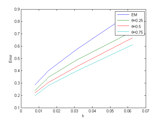
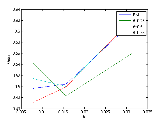
Table 1 presents a comparison between the $\theta$ - Euler-Maruyama technique and the Euler-Maruyama technique for the average values of the mean square error and the values of the strong convergence order. Additionally, curves Fig. 1(a) and Fig. 1(b) are displayed.

Stepsize	Euler-Maruyama method		$\theta$ -Euler-Maruyama method
	——————————		—————————————————————–
			$\theta=0.25$		$\theta=0.5$		$\theta=0.75$
	Error	Order	Error	Order	Error	Order	Error	Order
$2^{3}\Delta t$	0.36491		0.31615		0.24880		0.28555
$2^{4}\Delta t$	0.51287	0.49104	0.43569	0.46267	0.39184	0.45652	0.35430	0.50998
$2^{5}\Delta t$	0.72441	0.49822	0.62635	0.52368	0.54196	0.46794	0.49710	0.48856
$2^{6}\Delta t$	1.08861	0.58761	0.94770	0.59744	0.81481	0.58826	0.73190	0.55811

Table 1. The Means square errors and Strong convergence order of the Euler-Maruyama and

\theta

-Euler-Maruyama methods with

\theta\in[0.25,0.5,0.75]

for Example 5.1.

Refer to caption — (a) Mean square error of the Euler-Maruyama and $\theta$ -Euler-Maruyama method with $\theta\in[0.25,0.5,0.75]$ for Example 5.1.

The curves Fig. 1(a) and Fig. 1(b) showing the mean square error and strong convergence order curves of the Euler-Maruyama and $\theta$ -EM methods with $\theta=0.25,0.5,0.75$ , respectively, and based on the results presented in Table 1.

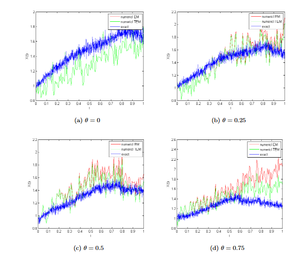
In Fig. 2, we have presented the solution curves. The blue curve shows the approximation of the analytic solution using the Euler-Maruyama method, the red curve shows the numerical solution of the Euler-Maruyama method, and the green curve shows the numerical solution of the $\theta$ -Euler-Maruyama method by changing the value of $\theta\left(\theta=0,\,0.25,\,0.5\text{ and }0.75\right),$ in proportion to Example 5.1.

Example 5.2.

In equation (5.15), we take $a=0.5,\hskip 5.69046ptb=0.2,\hskip 5.69046pt$ $\sigma_{1}(t,s)=\sin(2st-s),\hskip 5.69046pt\sigma_{2}=(t,s)=\cos(t^{2}-s+1).$

As with the previous example, we provided the main result of the second example by using the same approach. Table 2, corresponding to Example 5.2, presents the mean square error and the strong convergence results of the Euler-Maruyama and $\theta$ -Euler-Maruyama methods, and also reinforces the results obtained in Example 5.1.

Stepsize	Euler-Maruyama method		$\theta$ -Euler-Maruyama method
	——————————		—————————————————————–
			$\theta=0.25$		$\theta=0.5$		$\theta=0.75$
	Error	Order	Error	Order	Error	Order	Error	Order
$2^{3}\Delta t$	0,28632		0.23911		0,22111		0,19686
$2^{4}\Delta t$	0,40390	0,49637	0.34838	0.54296	0,30660	0,47154	0,28122	0,51449
$2^{5}\Delta t$	0,57300	0,50453	0.48685	0.48279	0,43328	0,49895	0,39785	0,50051
$2^{6}\Delta t$	0,87765	0,61508	0.71764	0.55977	0,66639	0,62105	0,61200	0,62130

Table 2. The Means square errors and Strong convergence order of the Euler-Maruyama and

\theta

-Euler-Maruyama methods with

\theta\in[0.25,0.5,0.75]

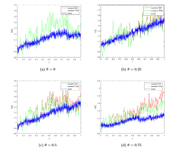
In Fig. 4, the solution curves are depicted. The blue curve represents the approximation of the analytical solution using the Euler-Maruyama method, the red curve represents the numerical solution of the Euler-Maruyama method, and the green curve represents the numerical solution of the $\theta$ -Euler-Maruyama method.

The strong convergence results of the $\theta$ -Euler-Maruyama method of stochastic Volterra integro-differential equations in Example 5.1 and Example 5.2 are shown in Table 1 and Table 2. From these tables, we can see that the $\theta$ -Euler-Maruyama method of the stochastic Volterra integro-differential equations (SVIDEs) is convergent of order 1/2.

6. Conclusion

In this paper, we examined a numerical solutions of a class of stochastic Volterra integro-differential equations. We investigated the existence, uniqueness, and Hölder continuity of the theoretical solution. Additionally, we considered the Euler-Maruyama (EM) and $\theta$ -EM methods for solving the SVIDEs, analyzing their mean-square error. Moreover, we established that the EM and $\theta$ -EM approximate solutions are strongly convergent with order around $1/2.$ Numerical examples have been provided to illustrate the effectiveness of the theoretical results obtained in this paper. As a result, we have shown that the $\theta$ -EM method is more efficient than the EM method for the numerical approximation of the solution of a stochastic Volterra integro-differential equations for different values of $\theta\,(\theta=0.25,0.5,0.75)$ .

References

[1] M. Bayram, T. Partal, and G. Orucova Buyukoz (2018) Numerical methods for simulation of stochastic differential equations. Advances in Difference Equations 2018, pp. 1–10. Cited by: §1.
[2] M. Bayram, T. Partal, and G. Orucova Buyukoz (2018) Numerical methods for simulation of stochastic differential equations. Advances in Difference Equations 2018, pp. 1–10. External Links: Link Cited by: §1.
[3] D. Conte, R. D’Ambrosio, B. Paternoster, et al. (2018) On the stability of $\vartheta$ -methods for stochastic volterra integral equations. Discr. Cont. Dyn. Sys.-Series B 23 (7), pp. 2695–2708. External Links: Link Cited by: §1.
[4] C. Deng and W. Liu (2020) Semi-implicit euler–maruyama method for non-linear time-changed stochastic differential equations. BIT Numerical Mathematics 60, pp. 1133–1151. External Links: Link Cited by: §1, §1, §1.
[5] S. Federico, G. Ferrari, and L. Regis (2020) Applications of stochastic optimal control to economics and finance. Basel: MDPI. External Links: Link Cited by: §1.
[6] D. J. Higham (2000) Mean-square and asymptotic stability of the stochastic theta method. SIAM journal on numerical analysis 38 (3), pp. 753–769. External Links: Link Cited by: §1.
[7] G. Lan, M. Zhao, and S. Qi (2022) Exponential stability of $\theta$ -em method for nonlinear stochastic volterra integro-differential equations. Applied Numerical Mathematics 172, pp. 279–291. External Links: Link Cited by: §1, §1, §1.
[8] M. Li, C. Huang, and Y. Hu (2022) Numerical methods for stochastic volterra integral equations with weakly singular kernels. IMA Journal of Numerical Analysis 42 (3), pp. 2656–2683. External Links: Link Cited by: §1.
[9] X. Mao and L. Szpruch (2013) Strong convergence and stability of implicit numerical methods for stochastic differential equations with non-globally lipschitz continuous coefficients. Journal of Computational and Applied Mathematics 238, pp. 14–28. Cited by: §1.
[10] X. Mao (2007) Stochastic differential equations and applications. Elsevier. Cited by: §1.
[11] K. Nouri, H. Ranjbar, and L. Torkzadeh (2019) Modified stochastic theta methods by odes solvers for stochastic differential equations. Communications in Nonlinear Science and Numerical Simulation 68, pp. 336–346. Cited by: §1.
[12] T. Sauer (2013) Computational solution of stochastic differential equations. Wiley Interdisciplinary Reviews: Computational Statistics 5 (5), pp. 362–371. External Links: Link Cited by: §1.
[13] W. Wang, L. Yan, S. Gao, and J. Hu (2021) The truncated theta-em method for nonlinear and nonautonomous hybrid stochastic differential delay equations with poisson jumps. Discrete Dynamics in Nature and Society 2021, pp. 1–17. External Links: Link Cited by: §1.
[14] X. Wang, J. Wu, and B. Dong (2020) Mean-square convergence rates of stochastic theta methods for sdes under a coupled monotonicity condition. BIT Numerical Mathematics 60 (3), pp. 759–790. External Links: Link Cited by: §1, §1.
[15] Z. Wang, Y. Gao, C. Fang, L. Liu, H. Zhou, and H. Zhang (2020) Optimal control design for connected cruise control with stochastic communication delays. IEEE transactions on vehicular technology 69 (12), pp. 15357–15369. External Links: Link Cited by: §1.
[16] H. Yang and F. Jiang (2014) Stochastic $\theta$ -methods for a class of jump-diffusion stochastic pantograph equations with random magnitude. The Scientific World Journal 2014. External Links: Link Cited by: §1.
[17] W. Zhang, H. Liang, and J. Gao (2020) Theoretical and numerical analysis of the euler–maruyama method for generalized stochastic volterra integro-differential equations. Journal of Computational and Applied Mathematics 365, pp. 112364. External Links: Link Cited by: §1, §1, §1, §2.
[18] X. Zong, F. Wu, and G. Xu (2018) Convergence and stability of two classes of theta-milstein schemes for stochastic differential equations. Journal of Computational and Applied Mathematics 336, pp. 8–29. External Links: Link Cited by: §1.

This work is licensed under a Creative Commons Attribution 4.0 International License.

	$\displaystyle\mathbb{E}\|Y_{n}(t)\|^{2}$	$\displaystyle\leq 3\mathbb{E}\|Y_{0}\|^{2}+3T\bigg{(}K^{\prime}T+K^{\prime}(1+%\lVert\sigma_{1}\rVert_{\infty}^{2}T)\displaystyle\int_{0}^{t}\mathbb{E}\|Y_{n}%(s)\|^{2}ds\bigg{)}$
		$\displaystyle\quad+3\bigg{(}K^{\prime}T+K^{\prime}(1+\lVert\sigma_{2}\rVert_{%\infty}^{2}T^{2})\displaystyle\int_{0}^{t}\mathbb{E}\|Y_{n}(s)\|^{2}ds\bigg{)}$
		$\displaystyle\leq 3\mathbb{E}\|Y_{0}\|^{2}+3K^{\prime}T(T+1)+3K^{\prime}T(1+%\lVert\sigma_{1}\rVert_{\infty}^{2}T)\displaystyle\int_{0}^{t}\mathbb{E}\|Y_{n}%(s)\|^{2}ds$
		$\displaystyle\quad+3K^{\prime}(1+\lVert\sigma_{2}\rVert_{\infty}^{2}T^{2})%\displaystyle\int_{0}^{t}\mathbb{E}\|Y_{n}(s)\|^{2}ds$
		$\displaystyle=3\mathbb{E}\|Y_{0}\|^{2}+3K^{\prime}T(T+1)+3K^{\prime}(C_{1}T+C_{2%})\displaystyle\int_{0}^{t}\mathbb{E}\|Y_{n}(s)\|^{2}ds,$

	$\displaystyle\mathbb{E}\|Y_{1}(t)-Y_{2}(t)\|^{2}=2\mathbb{E}\bigg{\|}%\displaystyle\int_{0}^{t}f\bigg{(}Y_{1}(u),\displaystyle\int_{0}^{u}\sigma_{1}%(u,s)Y_{1}(s)dB(s)\bigg{)}du$
	$\displaystyle\quad-\displaystyle\int_{0}^{t}f\bigg{(}Y_{2}(u),\displaystyle%\int_{0}^{u}\sigma_{1}(u,s)Y_{2}(s)dB(s)\bigg{)}du\bigg{\|}^{2}$
	$\displaystyle\quad+2\mathbb{E}\bigg{\|}\displaystyle\int_{0}^{t}g\bigg{(}Y_{1}(%u),\displaystyle\int_{0}^{u}\sigma_{2}(u,s)Y_{1}(s)ds\bigg{)}dB(u)-$
	$\displaystyle\quad-\displaystyle\int_{0}^{t}g\bigg{(}Y_{2}(u),\displaystyle%\int_{0}^{u}\sigma_{2}(u,s)Y_{2}(s)ds\bigg{)}dB(u)\bigg{\|}^{2}$
	$\displaystyle\leq 2T\displaystyle\int_{0}^{t}\mathbb{E}\bigg{\|}f\bigg{(}Y_{1}(%u)\displaystyle\int_{0}^{u}\sigma_{1}(u,s)Y_{1}(s)dB(s)\bigg{)}$
	$\displaystyle-f\bigg{(}Y_{2}(u),\displaystyle\int_{0}^{u}\sigma_{1}(u,s)Y_{2}(%s)dB(s)\bigg{)}\bigg{\|}^{2}du$
	$\displaystyle\quad+2\displaystyle\int_{0}^{t}\mathbb{E}\bigg{\|}g\bigg{(}Y_{1}(%u),\displaystyle\int_{0}^{u}\sigma_{2}(u,s)Y_{1}(s)ds\bigg{)}-g\bigg{(}Y_{2}(u%),\displaystyle\int_{0}^{u}\sigma_{2}(u,s)Y_{2}(s)ds\bigg{)}\bigg{\|}^{2}du$
	$\displaystyle\leq 2TK\displaystyle\int_{0}^{t}\bigg{(}\mathbb{E}\|Y_{1}(u)-Y_{2%}(u)\|^{2}+\displaystyle\int_{0}^{u}\mathbb{E}\bigg{\|}\sigma_{1}(u,s)\Big{(}Y_{%1}(s)-Y_{2}(s)\Big{)}\bigg{\|}^{2}ds\bigg{)}du$
	$\displaystyle\quad+2K\displaystyle\int_{0}^{t}\bigg{(}\mathbb{E}\|Y_{1}(u)-Y_{2%}(u)\|^{2}+u\displaystyle\int_{0}^{u}\mathbb{E}\bigg{\|}\sigma_{2}(u,s)\Big{(}Y_%{1}(s)-Y_{2}(s)\Big{)}\bigg{\|}^{2}ds\bigg{)}du$
	$\displaystyle\leq 2TK\displaystyle\int_{0}^{t}\bigg{(}\mathbb{E}\|Y_{1}(u)-Y_{2%}(u)\|^{2}+\lVert\sigma_{1}\rVert_{\infty}^{2}\displaystyle\int_{0}^{u}\mathbb{%E}\|Y_{1}(s)-Y_{2}(s)\|^{2}ds\bigg{)}du$
	$\displaystyle\quad+2K\displaystyle\int_{0}^{t}\bigg{(}\mathbb{E}\|Y_{1}(u)-Y_{2%}(u)\|^{2}+T\lVert\sigma_{2}\rVert_{\infty}^{2}\displaystyle\int_{0}^{u}\mathbb%{E}\|Y_{1}(s)-Y_{2}(s)\|^{2}ds\bigg{)}du$
	$\displaystyle\leq 2K\big{(}TC_{1}+C_{2}\big{)}\displaystyle\int_{0}^{t}\mathbb%{E}\|Y_{1}(s)-Y_{2}(s)\|^{2}ds$
	$\displaystyle\leq C\displaystyle\int_{0}^{t}\mathbb{E}\|Y_{1}(s)-Y_{2}(s)\|^{2}ds.$

	$\displaystyle\mathbb{E}\|Y_{n}(t)\|^{2}\leq$	$\displaystyle 3\mathbb{E}\|Y_{0}\|^{2}+3\mathbb{E}\bigg{\|}\int_{0}^{t}f\bigg{(}Y%_{n-1}(u),\int_{0}^{u}\sigma_{1}(u,s)Y_{n-1}(s)dB(s)\bigg{)}du\bigg{\|}^{2}$
		$\displaystyle+3\mathbb{E}\bigg{\|}\int_{0}^{t}g\bigg{(}Y_{n-1}(u),\int_{0}^{u}%\sigma_{2}(u,s)Y_{n-1}(s)ds\bigg{)}dB(u)\bigg{\|}^{2}$
	$\displaystyle\leq$	$\displaystyle 3\mathbb{E}\|Y_{0}\|^{2}+3T\bigg{(}K^{\prime}T+K^{\prime}(1+\lVert%\sigma_{1}\rVert_{\infty}^{2}T)\displaystyle\int_{0}^{t}\mathbb{E}\|Y_{n-1}(s)\|%^{2}ds\bigg{)}$
		$\displaystyle+3\bigg{(}K^{\prime}T+K^{\prime}(1+\lVert\sigma_{2}\rVert_{\infty%}^{2}T^{2})\displaystyle\int_{0}^{t}\mathbb{E}\|Y_{n-1}(s)\|^{2}ds\bigg{)}$
	$\displaystyle=$	$\displaystyle 3\mathbb{E}\|Y_{0}\|^{2}+3K^{\prime}T(T+1)+3K^{\prime}(C_{1}T+C_{2%})\displaystyle\int_{0}^{t}\mathbb{E}\|Y_{n}(s)\|^{2}ds$
	$\displaystyle=$	$\displaystyle 3\mathbb{E}\|Y_{n}(t)\|^{2}\leq 3\big{(}\mathbb{E}\|Y_{0}\|^{2}+C_{3%}\big{)}+3C\int_{0}^{t}\mathbb{E}\|Y_{n-1}(s)\|^{2}ds,$

	$\displaystyle\max_{1\leq k\leq n}\mathbb{E}\|Y_{k}(t)\|^{2}\leq$	$\displaystyle 3\big{(}\mathbb{E}\|Y_{0}\|^{2}+C_{3}\big{)}+3C\int_{0}^{t}\max_{1%\leq k\leq n}\mathbb{E}\|Y_{k-1}(s)\|^{2}ds$
	$\displaystyle\leq$	$\displaystyle 3\big{(}\mathbb{E}\|Y_{0}\|^{2}+C_{3}\big{)}+3C\int_{0}^{t}\bigg{[%}\mathbb{E}\|Y_{0}\|^{2}+\max_{1\leq k\leq n}\mathbb{E}\|Y_{k}(s)\|^{2}\bigg{]}ds$
	$\displaystyle\leq$	$\displaystyle 3\bigg{(}(1+CT)\mathbb{E}\|Y_{0}\|^{2}+C_{3}\bigg{)}+3C\int_{0}^{t%}\max_{1\leq k\leq n}\mathbb{E}\|Y_{k}(s)\|^{2}ds.$

	$\displaystyle\mathbb{E}\|Y_{1}(t)-Y_{0}(t)\|^{2}$	$\displaystyle=\mathbb{E}\|Y_{1}(t)-Y_{0}\|^{2}$
		$\displaystyle\leq 2\mathbb{E}\bigg{\|}\displaystyle\int_{0}^{t}f\bigg{(}Y_{0}(u%),\displaystyle\int_{0}^{u}\sigma_{1}(u,s)Y_{0}(s)dB(s)\bigg{)}du\bigg{\|}^{2}$
		$\displaystyle\quad+2\mathbb{E}\bigg{\|}\displaystyle\int_{0}^{t}g\bigg{(}Y_{0}(%u),\displaystyle\int_{0}^{u}\sigma_{2}(u,s)Y_{0}(s)ds\bigg{)}dB(u)\bigg{\|}^{2}$
		$\displaystyle\leq 2K^{\prime}\bigg{(}T(1+T)+\Big{(}T\underbrace{\big{(}1+T%\lVert\sigma_{1}\rVert_{\infty}^{2}\big{)}}_{C_{1}}+\underbrace{\big{(}1+T^{2}%\lVert\sigma_{2}\rVert_{\infty}^{2}\big{)}}_{C_{2}}\Big{)}\mathbb{E}\|Y_{0}\|^{2%}\bigg{)}:=C_{0},$

Convergence of the $\theta$ -Euler-Maruyama method for a class of Stochastic Volterra Integro-Differential Equations

Abstract.

Key words and phrases:

2005 Mathematics Subject Classification:

1. Introduction

2. Preliminaries

Definition 2.1.

Definition 2.2.

3. Theoretical analysis of the class of SVIDE

3.1. The existence and uniqueness of the analytical solution

Lemma 3.1.

Proof.

Theorem 3.1.

Proof.

3.2. Hölder continuity of the analytic solutions

Theorem 3.2.

Proof.

4. Numerical analysis of the class of SVIDE

4.1. $\theta$ -Euler Maruyama method

Remark 4.1.

Theorem 4.1.

Proof.

4.2. Strong convergence of the $\theta$ -Euler Maruyama method

Lemma 4.1.

Proof.

Theorem 4.2.

Proof.

5. Numerical experiments

Example 5.1.

Example 5.2.

6. Conclusion

References

Information

Indexing and abstracting

Publisher

Convergence of the θ-Euler-Maruyama method for a class of Stochastic Volterra Integro-Differential Equations

Abstract.

Key words and phrases:

2005 Mathematics Subject Classification:

1. Introduction

2. Preliminaries

Definition 2.1.

Definition 2.2.

3. Theoretical analysis of the class of SVIDE

3.1. The existence and uniqueness of the analytical solution

Lemma 3.1.

Proof.

Theorem 3.1.

Proof.

3.2. Hölder continuity of the analytic solutions

Theorem 3.2.

Proof.

4. Numerical analysis of the class of SVIDE

4.1. θ-Euler Maruyama method

Remark 4.1.

Theorem 4.1.

Proof.

4.2. Strong convergence of the θ-Euler Maruyama method

Lemma 4.1.

Proof.

Theorem 4.2.

Proof.

5. Numerical experiments

Example 5.1.

Example 5.2.

6. Conclusion

References

Information

Indexing and abstracting

Publisher

Convergence of the $\theta$ -Euler-Maruyama method for a class of Stochastic Volterra Integro-Differential Equations

4.1. $\theta$ -Euler Maruyama method

4.2. Strong convergence of the $\theta$ -Euler Maruyama method