ATM Transaction Simulation:
Combination of ACDs and Cox Process

Abstract.

Two main approaches for analyzing the ultra-frequency data such as ATM (auto teller machine) transaction are Cox process and autoregressive conditional durations (ACDs). This paper combines both models and gives its advantages. The functional data analysis proposes useful method for modeling the intensity of counting process. Two simulated cases results are verified. A real data set is analyzed and conclusions are also given.

1. Introduction

Irregularly spaced financial time series have received considerable attention in high-frequency data literature, see [6]. High frequency time series forecasting is a crucial field that tackles the analysis of data recorded at very short intervals, from seconds to fractions of a second. This discipline is fundamental in various sectors, from meteorology to finance, energy management, and quality control in manufacturing. Intraday transactions of ATM and POS [8], trading in stock markets [11], and volatility patterns in high frequency trading [9] are well-known examples of these time series. In the current paper, the ATM transactions are studied. To this end, suppose that $N(t)$ counts the number of intraday transactions of an ATM of a specific bank recorded up until time . Indeed, $N(t)$ is a counting process with intensity function $\Lambda (t)$.

There are two main independent approaches for analyzing these types of time series including the Cox Poisson process (referred as approach a, in this paper) from [11] and ACD models (approach b) from [4]. However, in the current paper, the combined approach (called approach c) is proposed. There, it is assumed that both types of Cox and ACD models govern on the data, simultaneously. According to the best author’s knowledge, this model is not applied before in the literature and has many advantages which are discussed in Section 2. Although, approaches a and b are customized for problem of in hand of the current paper.

$Approacha$: Cox process. Following [11], assume that $N(t)$ is modeled as Cox process. That is a Poisson process with a random intensity $\Lambda (t)$ where

$$\Lambda \left(t\right)={\int }_0^t\lambda \left(s\right)𝑑s.$$

The Cox process is a type of point process. For comprehensive review on Cox process and generally point processes, see [3].

Often, to find the functional forms of $\lambda$ and $\Lambda$, the functional data analysis (FDA) method is proposed which gives an approximation for $\lambda \left(t\right)$.

$Approachb$: ACD models. The ACD model mainly uses the stopping times of $N\left(t\right)$ and stopped process properties, without assuming $N(t)$ being a Poisson process, as Cox process assumes. To describe more, let ${\tau }_k$ be the time of $k$-th transaction (in a day)

$${\tau }_k={\inf }_t\left\{N\left(t\right)=k\right\}.$$

The related duration be $L_k$ defined by

$$L_k={\tau }_k-{\tau }_{k-1}.$$

Let $L_k$ be modeled by ACD model (with intercept $c$) from [4]; i.e.,

$$L_k=c+{\vartheta }_k{e}_k,$$

at which errors $e_k$’s are independent, positive random variables with $E\left(e_k\right)=1$ and

$${\vartheta }_k=\alpha +\sum _{j=1}^p{\gamma }_j{L}_{k-j}+\sum _{j=1}^q{\beta }_j{\vartheta }_{k-j},$$

where $p,q$ are unknown dimensions of model which are optimized during solving the case study problem while parameters ${\gamma }_j$ and ${\beta }_j$ are unknown parameters which should be estimated. The authors from [4] proposed a close relationship between ACD and GARCH models. The $ACDm$ package of software $R$ estimates these parameters, accurately and quickly, see [1].

$Approachc$: Combined model. Here, it is assumed that both models of Cox and ACD are hold, simultaneously. Some advantages of this approach are:

1. Under this setting, the exact Monte Carlo simulation for dynamics of $\lambda \left(t\right)$ is derived.

2. Often, FDA $\lambda \left(t\right)$ is a time-consuming task, because of choosing the length of linear combination of orthogonal basis function.

3. Choosing basis functions and number of them are a little subjective which is critical in applied problems.

4. By combined model, $N(t)$ is also simulated, directly, by Binomial distribution which approximates the Poisson distribution, see Section 2.3.

The rest of paper is organized as follows. In the next section, two methods are proposed to derive the dynamics of $\lambda \left(t\right)$. Section 3 gives the results of simulations. A real data set is analyzed in Section 4. Concluding remarks are proposed in Section 5.

2. Dynamics of $𝝀\left(𝒕\right)$

Here, dynamics of $\mathrm{\Lambda }\left(\mathrm{t}\right)$ and $\lambda \left(t\right)$are derived. To this end, first, the FDA method is proposed which gives an approximation for $\lambda \left(t\right)$. Then, under the combined model setting, the derivation of $\lambda \left(t\right)$ is based on Monte Carlo simulation which uses the exact distribution of partial sums of $L_k$’s.

2.1. FDA $𝝀\left(𝒕\right)$

In practice, FDA is used to model the intensity function $\lambda \left(t\right)$ of Poisson process as random element in Hilbert space, see [7]. To this end, considering $n$ days, let $N_i(t)$ the number of transactions throughout the $i$-th day with intensity function ${\lambda }_i\left(t\right)$. Following [8], to remove the periodically effects for different days, let ${\lambda }_i\left(t\right)$ be the intensity function of $i$-th day and let

$${\delta }_i\left(t\right)={\lambda }_i\left(t\right)-{\lambda }_{i-7}\left(t\right),$$

and consider the following functional autoregressive model for ${\delta }_i\left(t\right)$ as follows

$${\delta }_i\left(t\right)={\int }_0^1\rho (s,t){\delta }_{i-1}\left(s\right)𝑑s+{\epsilon }_i\left(t\right),$$

where kernel $\rho$ is estimated using the functional principal component and error terms

$$\{{\epsilon }_i\left(t\right);t\in [0,1]\}$$

are supposed to be independent functions such that $E\{{\epsilon }_i\left(t\right)\}=0$ for each $t\in [0,1]$ and

For comprehensive review on functional data analysis, see [10]. Package fda.usc of software $R$ is useful instrument for studying functional time series data, see [5]. Then, use the basis representation for $\lambda (t)$ such as

$$\lambda \left(t\right)=\sum _{k=1}^m{b}_k{\varphi }_k\left(t\right),$$

(see [10]) for basis functions ${\varphi }_k\left(t\right)$ for $k=1,\mathrm{\dots },m$, say Fourier basis functions. Therefore,

$$\Lambda \left(t\right)={\int }_0^t\sum _{k=1}^m{b}_k{\varphi }_k\left(s\right)ds=\sum _{k=1}^m{b}_k{\int }_0^t{\varphi }_k\left(s\right)𝑑s.$$

In the literature, widely used selections for ${\varphi }_k\left(t\right)$ are

However, in practice, we find $\widehat{\Lambda }(t)$ which we have

$$\widehat{\Lambda }\left(t\right)=\Lambda \left(t\right)+\zeta \left(t\right),$$

for some error terms $\zeta \left(t\right)$. Therefore,

$$\widehat{\Lambda }\left(t\right)=\sum _{k=1}^m{b}_k{\int }_0^t{\varphi }_k\left(s\right)𝑑s+\zeta \left(t\right).$$

Following [2], this is a type of functional regression analysis. To this end, variables $\widehat{\Lambda }\left(t_j\right)$ and ${\int }_0^{t_j}{\varphi }_k\left(s\right)𝑑s$ are computed for $t=t_j;j=1$,…,$M$, () and parameters of a multiple regression model are estimated.

2.2. $𝝀\left(𝒕\right)$ in combined model

Here, the exact functional form of $\lambda (t)$ is derived. To this end, let $L_0={\tau }_0=0$ and

$${\tau }_k=\sum _{j=1}^k{L}_j.$$

Notice that

$$P\left({\tau }_k\le t\right)=P(N\left(t\right)>k).$$

Hence,

$$P\left({\tau }_{k-1}\le t\right)=P(N\left(t\right)>k-1).$$

Let $p_k\left(t\right):=P\left(N\left(t\right)=k\right)$. One can see that

$$p_k\left(t\right)=P\left(N\left(t\right)>k-1\right)-P\left(N\left(t\right)>k\right)=P\left({\tau }_{k-1}\le t\right)-P\left({\tau }_k\le t\right).$$

It is concluded that

$$p_k\left(t\right)=P\left(\sum _{j=1}^{k-1}{L}_j\le t\right)-P\left(\sum _{j=1}^k{L}_j\le t\right).$$

This relation leads to the computation of the exact probabilities. Notice that

Therefore, the Monte Carlo estimate of $p_k(t)$ is the number of times (in M repetitions of Monte Carlo simulations) that the random interval

$$[\sum _{j=1}^{k-1}{L}_j;\sum _{j=1}^k{L}_j)$$

contains the constant number $t$. In practice, after fitting and $ACD(p,q)$ to $L_k$, the Monte Carlo simulation method approximates the exact distribution of ${\sum }_{j=1}^k{L}_j$ and ${\sum }_{j=1}^{k-1}{L}_j$, hence $P\left(N\left(t\right)=k\right)$ is computed. Notice that

$$k!p_k\left(t\right)=\exp (-\mathrm{\Lambda }\left(\mathrm{t}\right)){\Lambda }^k\left(\mathrm{t}\right).$$

Therefore,

$$\mathrm{\Lambda }\left(\mathrm{t}\right)-k\log \left(\mathrm{\Lambda }\left(\mathrm{t}\right)\right)+b_k\left(t\right)=0,$$

where

$$b_k\left(t\right)=\log (k!p_k\left(t\right)).$$

This is a non-linear equation and root-finding methods such as Newton-Raphson are applicable, as follows: For iteration $r$-th, let

$${\mathrm{\Lambda }}_r\left(t\right)={\mathrm{\Lambda }}_{r-1}\left(t\right)+\frac{{\mathrm{\Lambda }}_{r-1}\left(t\right)-k\log \left({\mathrm{\Lambda }}_{r-1}\left(t\right)\right)+b_k\left(t\right)}{1-k/{\mathrm{\Lambda }}_{r-1}\left(t\right)}.$$

To find $\lambda \left(t\right),$ after finding $\Lambda (t)$ for discrete values of $t$’s, the numerical differentiation is applied to find discrete values of $\lambda (t)$. Then, a smoothing method such as spline or smoothing polynomials is used to derive the functional form of $\lambda (t)$.

2.3. Another combined $𝝀\left(𝒕\right)$

In Sections 2.1 and 2.2, we proposed some methods for obtaining functional form of $\lambda (t)$ based on Cox process and ACD models. However, in practice, the series of numbers of events that each occurred in small fraction of the time are recorded and it is necessary to simulate $N(t)$, itself, directly.

The idea behind this method is that the Binomial distribution approximates the Poisson distribution. To propose the method, suppose that throughout a crowded business day which is expected the possible numbers of $t$’s in $(t-h,t)$ where at them transaction occur i.e., $n$ (of Bernoulli distribution) is large. However, because of some political or social events which has happened in yesterday, the probability of transaction $p_t$ is too low such that

$$n{p}_t\approx {\int }_{t-h}^h\lambda \left(s\right)𝑑s.$$

Following [8] and noticing that

$${\int }_{t-h}^h\lambda \left(s\right)𝑑s\approx h\lambda \left(t\right),$$

it is seen that $\frac{1}{h}n{p}_t$ is a good estimate of $\lambda \left(t\right)$. Therefore, $N\left(t\right)$ is simulated by sampling from binomial distribution with parameter $(n,p_t)$, directly and

$$\lambda \left(t\right)=\frac{1}{h}n{p}_t.$$

Then, by collecting number of transactions and fitting an ACD model, the empirical estimate of $N(t)$ and consequently $p_t$ are estimated.

Suppose that, the dynamic of $p_t$ is proposed. For example, consider the dynamics of $p_t$ given by Ito stochastic differential equation, as follows:

$$d{p}_t=\alpha p_{t}dt+\delta p_{t}d{B}_t,$$

where $B_t$ is standard Brownian motion on (0,1). To obtain parameters $\alpha ,\delta$, notice that they are mean and standard deviation of $\frac{d{p}_t}{p_{t}dt}$ which are estimated by their related samples values. Therefore, the dynamic of $\lambda \left(t\right)$ is proposed.

3. Simulations

In this section, some simulated cases are analyzed. Banks often refuse to provide tick-by-tick transaction data of ATMs and do not make this type of data available (or at least hard available) to the public due to network security issues and keeping customer’s secrets. However, a small part of database is usually given to researchers from the core system of databases of banks. This is why, in the current paper, we only survey the simulated situations which correspond to real data. For using simulated data instead of real one, we must be sure that the simulated data with the combined model are good approximations for the real data. However, since in both cases, we use the dataset in [11], we are sure that these considerations are checked. Case 1 studies the Cox process with known dynamic for $\lambda$. Case 2 gives simulation results under the combined model setting.

Case 1: $\lambda (t)$ as OU process. In the Cox process, motivated by [11], suppose that $\lambda (t)$ is an Ornstein-Uhlenbeck (OU process) process defined by

$$d\lambda \left(t\right)=-\beta \lambda \left(t\right)dt+\beta tdz,$$

where $dz$ is increment of Brownian motion, $t\in (0,1)$ and . Here, it is supposed that $\beta =0.2$ which corresponds to the empirical results from [11]. Consider $t_i=\frac{i}{100},i=0,\mathrm{\dots },99$ and let $\Lambda \left(t_i\right)=\frac{1}{100}{\sum }_{u=1}^b\lambda (u),$ where $b=[100t_i]$. To simulate $N(t)$ at $t_i$’s, increments $N\left(t_i\right)-N(t_{i-1})$ are samples from Poisson distribution with rate $\frac{1}{100}{\sum }_{u=a}^b\lambda (u)$ where $a=\left[100t_{i-1}\right].$ In this way, the partial sums of increments generate paths of Poisson process. Therefore, $L_k$’s are computable. It is easy to see that $L_k$ is $ACD(1,1)$ process with intercept, as follows

$$L_k=0.0898+{\vartheta }_k{e}_k,$$

where $e_k$ has exponential distribution with mean 1 and

$${\vartheta }_k=0.0017+0.885e_{k-1}-1.58{\vartheta }_{k-1}.$$

Case 2: Combined $\lambda (t)$. Here addition to Cox process assumption, assume that $L_k$ come from process $ACD(1,1)$. For the weekly data from [11], the ACD model is defined by

$$L_k=0.01+{\vartheta }_k{e}_k,$$

$${\vartheta }_k=0.002+0.65e_{k-1}-2{\vartheta }_{k-1},$$

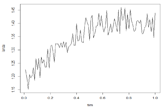
with $e_k$ being exponentially distributed random variable with rate 1. Hence, empirical distributions of $L_k,k=1,2$ are computed. Next, using the Monte Carlo method proposed in subsection 2.1, $P(N\left(t\right)=2)$ is computed for various values of $t_i$’s. Then, using the Newton-Raphson and numerical differentiation, values of $\Lambda (t)$ and $\lambda (t)$ are computed, respectively. The following figure gives the plot of $\lambda (t)$. Smoothing $\lambda (t)$ by basis Fourier function, it is seen that

$$\lambda \left(t\right)=\left(1+\sin \left(t\right)+\cos \left(t\right)\right)/\sqrt{\pi }.$$

Figure 1. Plot of $\lambda (t)$

Although it is difficult to obtain real tick-by-tick data in practice, nevertheless, the case 3 provides an alternative method for reconstructing$\lambda (t)$. For the weekly data from [11], the following smoothing results are provided:

$${\lambda }_i\left(t\right)=\left(c_{0i}+c_{1i}\sin \left(t\right)+c_{2i}\cos (t)\right)/\sqrt{\pi },$$

where $\pi =3.141592$ and $c_{ji},j=0,1,2$ are periodic functions with period 7 given as follows:

$i$	1	2	3	4	5	6	7
$c_{0i}$	0.2	0.2	0.5	0.5	0.1	0.25	0.25
$c_{1i}$	0.1	0.1	0.5	0.25	0.5	0.2	0.5
$c_{2i}$	0.2	0.2	0.1	0.1	0.1	0.25	0.25

Table 1. Values of $c_{ji}$ for $j=0,1,2$ and $i=1,\mathrm{\dots },7$.

4. Real data sets

Here, the method of Section 2.3 is applied to 3 real-time series.

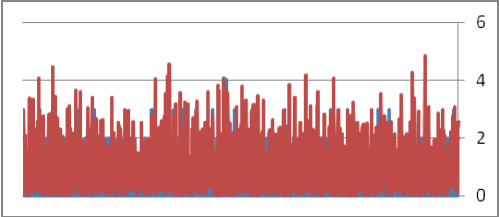
Data set 1. The dataset includes 11520 observations which are 15-minute by 15-minute ATM transactions of a selected branch of an Iranian Bank ABC (which we are not naming for security reasons) from March 11, 2024 to October 11 2024 (30 days) during 7 AM to 7 PM. For a day, there are $n=48$ 15 minutes. Therefore, $h=1/48$. Thus, $\lambda \left(t\right)=p_t$. The time series plot of first 5000 observations is given as follows:

Figure 2. (a) Plot of $\lambda (t)$; (b) Time series of $N(t)$.

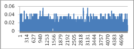
It is seen that $\alpha =0.641,\delta =0.457$. Here, we provide fittings of the model on many real high frequency data sets, then obtain the optimal parameters, plot on the same figure the real data and the optimal model and last analyze the corresponding residuals. The following plot gives the simultaneously, time series of actual $\lambda \left(t\right)$ (blue line) and its estimate (red line).

Figure 3. Plot of $\lambda (t)$ and its estimate.

The following table gives the max, min, mean and standard deviation (sd) of 5000 residuals

$$\left|\frac{\lambda \left(t\right)}{est(t)}-1\right|.$$

The table shows that errors are negligible.

Max	Min	Mean	SD
0.0632	0.0024	0.0414	0.019

Table 2. Residuals properties: maximum, minimum, mean, and standard deviation.

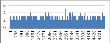
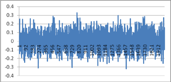
Data set 2. In the second data set, the transactions of an ATM along one day for 6336 days are recorded. First the following ACD model is fitted to duration of transactions

$$L_k=0.045+{\vartheta }_k{e}_k,$$

$${\vartheta }_k=0.001+0.34e_{k-1}-1.68{\vartheta }_{k-1},$$

$k=1,2,\mathrm{\dots },6336$. The following plot gives real $N(t)$ is plotted against its estimated process derived from above ACD model using simulation of a Poisson process based on simulating the $L_k$’s partial sums. To better presentation the first 3000 observations i.e., the actual $N\left(t\right)$ (blue line) and its estimate (red line) are presented. This figure shows the maximum closeness of both series.

Figure 4. Plot of $N(t)$ and its estimate.

Again, the summaries of errors are proposed in the following table.

Max	Min	Mean	SD
0.0475	0.0064	0.0325	0.032

Table 3. Differences between $N(t)$ and its estimate: maximum, minimum, mean, and standard deviation.

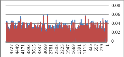
Also, a Poisson process is fitted to data, based on functional estimate of $\lambda \left(t\right)$, given by

$$\lambda \left(t\right)=(0.01+0.002\sin \left(t\right)+0.25\cos (t))/\sqrt{2\pi }.$$

The following table gives the related errors.

Max	Min	Mean	SD
0.0734	0.0055	0.0455	0.043

Table 4. Differences between actual $N(t)$ and its Poisson simulation: maximum, minimum, mean, and standard deviation.

Data set 3. Here, the functional form of $\lambda \left(t\right)$ of previous data set are compared with its actual values. First the following table shows that the errors are negligible. Then, different scenarios are studied using 1 times standard deviations of errors as shocks to $\lambda \left(t\right)$. The following figure shows the errors of actual $\lambda \left(t\right)$ and its functional estimates. Shocks are simulated using normal distributions with zero means and 1 times standard deviations.

Figure 5. Plot of errors between $\lambda (t)$ and its estimate.

Figure 6. Plot of $\lambda (t)$ and its shock estimate.

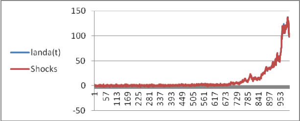
As seen, the shocks increase as the number of time series increases. However, the shocks are negligible in the estimate of $\lambda \left(t\right)$.

5. Concluding Remarks

This manuscript has many advantages and highlights as follows:

1. The compatibility of the combination of two common models used in the analysis of data with high frequency was examined and it was seen in the simulation section that these two models can be recovered from each other.

2. The use of functional data analysis was used as a practical solution for modeling the intensity function of the Poisson process, and the performance of this solution was seen alongside the previous two methods.

3. Mathematical models were developed to be useful for simulation analysis.

Acknowledgements.

The author thanks the referees and the editor for their useful remarks, which contributed to improving the quality of this article.