Falkner Hybrid Block Methods for Second-Order IVPs:
A Novel Approach to Enhancing Accuracy and Stability Properties

Abstract.

Second-order initial value problems (IVPs) in ordinary differential equations (ODEs) are ubiquitous in various fields, including physics, engineering, and economics. However, their numerical integration poses significant challenges, particularly when dealing with oscillatory or stiff problems. This article introduces a novel Falkner hybrid block method for the numerical integration of second-order IVPs in ODEs. The newly developed method is of order six with a large interval of absolute stability and is implemented using a fixed step size technique. The numerical experiments show the accuracy of our methods when compared with Falkner linear multistep methods, block methods, and other hybrid codes proposed in the scientific literature. This innovative approach demonstrates improved accuracy and stability in solving second-order IVPs, making it a valuable tool for researchers and practitioners.

1. Introduction

Ordinary differential equations (ODEs) are prevalent in various scientific disciplines, allowing for the modeling of temporal and spatial changes in a wide range of scenarios. Practical applications of ODEs include predicting the movement of electricity, analyzing the oscillatory motion of objects like pendulums, and explaining principles of thermodynamics. In medicine, ODEs are used to estimate disease progression visually. The general $n$th-order ODE can be written as,

(1) $$y^{(n)}=f(x,y,y^{\prime },\mathrm{\dots },y^{(n-1)})$$

Solving (1) often involves converting it into a system of first-order equations and using the appropriate method to solve the system, (see, [8], [18], [19], [22], and [25]). [9] noted that this process can be time-consuming, especially when developing a computer program. In addition to the main program, separate programs for initial values and functions from the equation system are typically required. This complexity may discourage newcomers from exploring promising numerical methods due to a lack of knowledge and confidence in crafting programs to validate their results.

The second-order IVPs in ODEs that we aim to approximate on a given interval in this research stem from (1) when $n$ = 2, resulting in the following IVPs,

(2) $$\{\begin{array}{cc}{y}^{\prime \prime }(x)=f(x,y(x),y^{\prime }(x)),\hfill & \\ y(0)=y_0,y^{\prime }(0)=y_0^{\prime },\hfill & \\ x\in [x_0,x_n].\hfill & \end{array}$$

where $y\in R^N$ and $f:R\times R\times R^N\to R^N$ are continuous vector-valued functions. The theoretical solutions to (1.2) are usually highly oscillatory. Second-order IVPs are fundamental in modeling various phenomena, such as oscillations, vibrations, and electrical circuits. However, their numerical integration requires careful consideration of accuracy, stability, and efficiency. The earlier proposed schemes for the direct solution of second-order ODEs (2) in literature can be found in the articles of the authors: [1], [2], [3], [4], [5], [6], [7], [9], [10], [11]-[13], [14], [15], [16], [17], [18], [19], [20], [21], [22], [23], [24], [25], [26], [28], [29], and [30]. In this article we formulate and derive a family of Falkner hybrid block methods with off-step points, using interpolation and collocation techniques. The proposed scheme modifies the Falkner block method in [29].

The paper is organized as follows: In Section 2, we reviewed the Falkner block method in [29]. Section 3 deals with the formulation and the derivation of the Falkner hybrid block method with an off-step point of order $k$ + 2. In Section 4, we give the main properties of the proposed method. Section 5 is devoted to the numerical experiments of the method. We compared the accuracy of our methods with other methods proposed in the literature. Finally, Section 6 is dedicated to conclusion.

2. Review of the Falkner Method and its Block Form

Falkner method (FM) was introduced by V. M Falkner in 1936. This scheme was for the numerical solution of second-order ODEs. The general form of a couple $k$-step Falkner method is,

(3) $$\{\begin{array}{cc}{y}_{n+k}=y_{n+k-1}+h{y}_{n+k-1}^{\prime }+h^2{\sum }_{j=0}^k{\beta }_j{f}_{n+j},\hfill & \\ y_{n+k}^{\prime }=y_{n+k-1}^{\prime }+h{\sum }_{j=0}^k{\overline{\beta }}_j{f}_{n+j}.\hfill & \end{array}$$

where, $y_{n+k}=y(x_{n+k})$, and $y_{n+k}^{\prime }=y^{\prime }(x_{n+k})$ are approximations to the solutions and its derivative at $x_n=x_0+nh$, and $f(x_{n+j},y_{n+j})$ = $y_{n+j}^{\prime \prime }$ is the function emanating from the second order ODEs. The h denotes the step size, $k$ represents the step number and ${\beta }_j$ is a constant parameter. The algorithm in (3) is: (i). explicit, if ${\beta }_k=0$ and (ii) implicit, if ${\beta }_k\ne 0$. A subclass of the formula in (3) is the explicit Falkner method in [14] and the two implicit Falkner schemes in [20].

The Falkner method is another form of hybrid method, it combines different numerical methods, to solve second-order boundary value problems (see [17] and [29]). The block form of the Falkner method in (3) is,

(4) $$A{Y}_n=hB{Y}_n^{\prime }+h^{2}C{F}_n,$$

where $A,B,$ and $C$ are matrices of coefficients of dimension 2$k$ by ($k$+1), and

(5) $$Y_n=\left(\begin{array}{c}{y}_n\\ \mathrm{⋮}\\ y_{n+k-1}\\ y_{n+k}\end{array}\right),Y_n^{\prime }=\left(\begin{array}{c}{y}_n^{\prime }\\ \mathrm{⋮}\\ y_{n+k-1}^{\prime }\\ y_{n+k}^{\prime }\end{array}\right),F_n=\left(\begin{array}{c}{f}_n\\ \mathrm{⋮}\\ f_{n+k-1}\\ f_{n+k}\end{array}\right).$$

The theoretical solution to (5) is the vectors,

(6)

The associated local truncation error of the methods in (5) is,

(7) $$E_n[y(x_n);h]=A{\mathrm{\Psi }}_n-hB{\mathrm{\Psi }}_n^{\prime }-h^{2}C{\mathrm{\Psi }}_n^{\prime \prime },$$

where $A,B,C$ are matrices of coefficients of dimension 2$k$ by ($k$+1). The block method in (4) and the associated linear difference operator in (7) is said to be of order $p$ if after expanding (6) by Taylor series about $x_n$ and inserting the resulting expressions into (7) we obtain

(8) $$\Vert E_n[y(x_n);h]\Vert =\overline{C}{h}^{p+2}+𝒪(h^{p+3}),$$

$\parallel \cdot \parallel$ may be the maximum norm we adopted for convenience.

To determine whether a numerical formula will yield realistic results as step size $h$ becomes large, there is a need for more insight into the types of stability properties the method processes with zero stability being one of them. In most numerical schemes proposed for solving second-order ODEs, the stability properties are generally investigated by considering the linear test equation in [25],

(9) $$y^{\prime \prime }(x)=-{\mu }^{2}y(x),\mu \ge 0.$$

Recall that the second-order ODEs in (2) contain the first derivative component, but the [25] test equation, does not contain the first derivative component $y^{\prime }(x)$, thus, a generalized test equation that includes the first derivative component, $y^{\prime }(x)$, as in ODEs (2) is,

(10) $$y^{\prime \prime }(x)=-{\mu }^{2}y(x)-2\mu y^{\prime }(x),\mu \ge 0,$$

which has bounded solutions for $\mu \ge 0$ that tend to zero as $x\to \mathrm{\infty }$ and this shall be the test equation for the stability analysis in this article. For further reading, see [29].

Definition 1.

Zero stability is concerned with the stability of the difference system in the limit as $h$ tends to 0. Thus as $h\to$ 0, the difference system in Equation (2) becomes

$$A^{(0)}{Y}_m-A^{(1)}{Y}_{m-1}=0,$$

where $A^{(0)}=I$, and $I$ is an identity matrix of order $k$, and $A^{(1)}$ is a coefficient matrix of order $k$.

Definition 2 ([18]).

A block method (4) is zero-stable if the roots of the first characteristic polynomial have modulus less than or equal to one and those of modulus one do not have multiplicity greater than $2$, i.e., the roots of

$$\rho (w)=det[Iw-A^{(0)}]=0,$$

satisfy $|w_j|\le 1$ and for those roots with $|w_j|=1$, the multiplicity does not exceed $2$. Since $\rho (w)=(w-1)w^{k-1}$ the block method in (4) is zero-stable.

Definition 3.

The block method in (4) is $p$-stable if its interval periodicity is $(0,\mathrm{\infty })$.

An example of the two-step Falkner method in [29] is,

(11) $$\{\begin{array}{cc}{y}_{n+2}=y_{n+1}+h{y}_{n+1}^{\prime }+\frac{h^2}{24}(3f_{n+2}+10f_{n+1}-f_n),\hfill & \\ y_{n+2}^{\prime }=y_{n+1}^{\prime }+\frac{h}{12}(5f_{n+2}+8f_{n+1}-f_n),\hfill & \\ y_n=y_{n+1}-h{y}_{n+1}^{\prime }+\frac{h^2}{24}(3f_n+10f_{n+1}-f_{n+2}),\hfill & \\ y_n^{\prime }=y_{n+1}^{\prime }-\frac{h}{24}(5f_n+8f_{n+1}-2f_{n+2}).\hfill & \end{array}$$

The methods in (11) have order $p$ = 3 respectively. The block form of the schemes in (11) is,

(12)

Applying (12) to (10) after eradicating the first derivatives yields the stability polynomial,

(13)

Plotting the roots of the stability polynomial in (13) via boundary locus sense gives the interval of absolute stability of the scheme in (12) as (0, 1.73205).

3. The Falkner Hybrid Block (FHB) Methods

In this section, we introduce Falkner hybrid methods for the numerical solution of ODEs in (2). The proposed method modifies the Falkner method discussed in [29]. The general form of the proposed FHM is

(14a) $$y_{n+c_i}={\alpha }_{k0}(c_i)y_{n+k-1}+{\alpha }_{k1}(c_i)h{y}_{n+k-1}^{\prime }+h^2\sum _{j=0}^k{\beta }_{kj}{f}_{n+j}(c_i)+h^2{\beta }_v{f}_{n+v}(c_i),$$

(14b) $$y_{n+c_i}^{\prime }={\varphi }_{k0}(c_i)y_{n+k-1}^{\prime }+h\sum _{j=0}^k{\overline{\beta }}_{kj}{f}_{n+j}(c_i)+h{\overline{\beta }}_v{f}_{n+v}(c_i),i=0,1,2,\mathrm{\dots }r,$$

$$c={(c_1,c_2,\mathrm{\dots },c_{r-1},c_r)}^T,c\in [k-1,k],c_{r-1}=v,c_i=(x-x_n)/h,$$

where . The ${\alpha }_{k0}(c_i)$, ${\alpha }_{k1}(c_i)$, ${\{{\beta }_{kj}(c_i)\}}_{j=0}^k$, ${\beta }_v(c_i)$, ${\varphi }_{k0}(c_i)$, ${\{{\overline{\beta }}_{kj}\}}_{j=0}^k(c_i)$ and ${\overline{\beta }}_v(c_i)$ are the continuous coefficients of the method, $c$ is the abscissa vector, $c={(c_1,c_2,\mathrm{\dots },c_{r-1},c_r)}^T$, and $h$ is the step size. The output points are $y_{n+c_i}$ and $y_{n+c_i}^{\prime }$. Also, in (14), $y_{n+c_i}^{\prime }$ and $y_{n+k-1}^{\prime }$ are the first derivative component while ${\{y^{\prime \prime }(x_{n+j})\}}_{j=0}^k={\{f(x_{n+j},y_{n+j},y_{n+j}^{\prime })\}}_{j=0}^k$ and $y^{\prime \prime }(x_{n+v})=f(x_{n+v},y_{n+v},y_{n+v}^{\prime })$ is the second derivative function. The $v$ in formula (14) is the hybrid point (i.e., off-step point). if $c_i=v$ in (14) a new hybrid LMM is defined. The block form of the Falkner hybrid methods in (14) is,

(15) $$A{Y}_{n+c}=hB{Y}_{n+c}^{\prime }+h^{2}C{F}_{n+c},$$

where $c={(c_0,c_1,\mathrm{\dots },c_{r-1},c_r)}^T$, is the abscissa vector, $A,B,$ and $C$ are the coefficients matrices of dimension 2$k$+2 by ($k$+2), and the vectors,

(16) $$Y_{n+c}=\left(\begin{array}{c}{y}_{n+c_0}\\ \mathrm{⋮}\\ y_{n+c_{r-1}}\\ y_{n+c_r}\end{array}\right),Y_{n+c}^{\prime }=\left(\begin{array}{c}{y}_{n+c_0}^{\prime }\\ \mathrm{⋮}\\ y_{n+c_{r-1}}^{\prime }\\ y_{n+c_r}^{\prime }\end{array}\right),F_{n+c}=\left(\begin{array}{c}{f}_{n+c_0}\\ \mathrm{⋮}\\ f_{n+c_{r-1}}\\ f_{n+c_r}\end{array}\right).$$

The theoretical solution to (15) is the vectors,

(17)

The associated local truncation error of the methods in (15) is,

(18) $$E_n[y(x_n);h]=A{\mathrm{\Psi }}_{n+c}-hB{\mathrm{\Psi }}_{n+c}^{\prime }-h^{2}C{\mathrm{\Psi }}_{n+c}^{\prime \prime }.$$

The block hybrid multistep method in (15) and the associated linear difference operator in (18) are said to be of order $p$ if after expanding (17) by Taylor series about $x_n$ and inserting the resulting expressions into (18) we obtain

(19) $$\parallel E_n[y(x_n);h\parallel =\overline{C}{h}^{p+2}+𝒪(h^{p+3}),$$

where $\overline{C}$ is the error constant of the method in (15) and $\parallel \cdot \parallel$ is the maximum norm we adopted for convenience.

4. Construction of the Falkner Hybrid Method

This subsection introduces the derivation of the Falkner hybrid method in (14). To do this we use the following polynomial interpolant,

(20) $$y(x)=\sum _{j=0}^N{a}_j{x}^j,$$

Differentiating (20) with respect to $x$ yields

(21) $$y^{\prime }(x)=\sum _{j=1}^{N}j{a}_j{x}^{j-1},$$

Again, differentiating (21) with respect to $x$ gives,

(22) $$y^{\prime \prime }(x)=f(x,y,y^{\prime })=\sum _{j=2}^{N}j(j-1)a_j{x}^{j-2},$$

Collocating (21) at $x=x_{n+j}$, $j$ = 0 (1) $k$, and $x$ = $x_{n+v}$, and interpolating (22) at $x$ = $x_{n+k-1}$, results in the linear system of equations,

(23) $$X_1{\mathrm{\Theta }}_1={\mathrm{\Omega }}_1$$

where

$${\mathrm{\Theta }}_1=\left(\begin{array}{ccccc}{a}_0& & & & \\ a_1& & & & \\ a_2& & & & \\ \mathrm{⋮}& & & & \\ a_{N-1}& & & & \\ a_N& & & & \end{array}\right);{\mathrm{\Omega }}_1=\left(\begin{array}{cccccc}{y}_{n+k-1}& & & & & \\ y_{n+k-1}^{\prime }& & & & & \\ f_n& & & & & \\ \mathrm{⋮}& & & & & \\ f_{n+k}& & & & & \\ f_{n+v}& & & & & \end{array}\right).$$

We obtained the value of $a_j^{\prime }s$ by the Gaussian elimination method. Substituting the resulting values of $a_j^{\prime }s$, ($j=0(\text{<a href="\#S1.E1" title="Equation 1 ‣ 1. Introduction ‣ Falkner Hybrid Block Methods for Second-Order IVPs: A Novel Approach to Enhancing Accuracy and Stability Properties" class="ltx\_ref ltx\_font\_italic"><span class="ltx\_text ltx\_ref\_tag">1</span></a>})N$) with $x=x_n+c_{i}h$, $i=0(\text{<a href="\#S1.E1" title="Equation 1 ‣ 1. Introduction ‣ Falkner Hybrid Block Methods for Second-Order IVPs: A Novel Approach to Enhancing Accuracy and Stability Properties" class="ltx\_ref ltx\_font\_italic"><span class="ltx\_text ltx\_ref\_tag">1</span></a>})r$ (without loss of generality we set $x_n=0$ so that $x=c_{i}h$) into (19) yields the continuous formulas in (14a).

Inserting the value of $c={(c_0,c_1,\mathrm{\dots },c_{r-1},c_r)}^T$ into the continuous formulas gives the discrete form of (14a). Similarly, to obtain the second method (14b), collocate (22) at $x=x_{n+j}$, $j=0(\text{<a href="\#S1.E1" title="Equation 1 ‣ 1. Introduction ‣ Falkner Hybrid Block Methods for Second-Order IVPs: A Novel Approach to Enhancing Accuracy and Stability Properties" class="ltx\_ref ltx\_font\_italic"><span class="ltx\_text ltx\_ref\_tag">1</span></a>})k$, and $x=x_{n+v}$ and interpolate (21) at $x=x_{n+k-1}$ gives the linear system of equations

(24) $$X_2{\mathrm{\Theta }}_2={\mathrm{\Omega }}_2$$

where

$${\mathrm{\Theta }}_2=\left(\begin{array}{ccccc}{a}_0& & & & \\ a_1& & & & \\ \mathrm{⋮}& & & & \\ a_{N-1}& & & & \\ a_N& & & & \end{array}\right);{\mathrm{\Omega }}_2=\left(\begin{array}{cccccc}{y}_{n+k-1}^{\prime }& & & & & \\ f_n& & & & & \\ \mathrm{⋮}& & & & & \\ f_{n+k}& & & & & \\ f_{n+v}& & & & & \end{array}\right).$$

Following the above procedures we obtain the formula in (14b).

4.1. The Falkner hybrid block method of order $p=k$+2 for $k$ = 4 steps

In the spirit of [27], and [29], we fix $k$ =4 in (23) and $N$ = 7 in (20), (21), and (22). Following the process in Section 4 gives the continuous formulas in (14) Inserting $v=\frac{11}{3}$ and $c={(0,1,2,\frac{11}{3},4)}^T$ into the resulting continuous method in (14) gives the discrete form of (14). Casting the resulting discrete schemes in block format yields the Falkner hybrid block methods in (15) for step number $k$ = 4, with the coefficient matrices as,

(25)

and the vectors as,

$$Y_{n+c}=\left(\begin{array}{c}{y}_n\\ y_{n+1}\\ y_{n+2}\\ y_{n+3}\\ y_{n+\frac{11}{3}}\\ y_{n+4}\end{array}\right);Y_{n+c}^{\prime }=\left(\begin{array}{c}h{y}_n^{\prime }\\ h{y}_{n+1}^{\prime }\\ h{y}_{n+2}^{\prime }\\ h{y}_{n+3}^{\prime }\\ h{y}_{n+\frac{11}{3}}^{\prime }\\ h{y}_{n+4}^{\prime }\end{array}\right);F_{n+c}=\left(\begin{array}{c}{f}_n\\ f_{n+1}\\ f_{n+2}\\ f_{n+3}\\ f_{n+\frac{11}{3}}\\ f_{n+4}\end{array}\right);$$

The Falkner hybrid block method in (15) is of order $p=6$ with error constant,

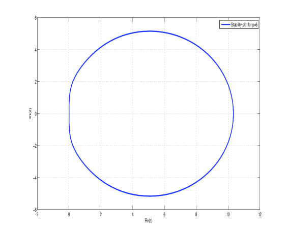
We obtain four stability polynomials by applying the order $p=6$ Falkner hybrid block method in (15) to the generalized test equation (10) and eliminating the derivatives using the Eliminate package in Mathematica. Due to their size, these polynomials are omitted. The boundary locus shows that the Falkner hybrid block method in (15) is stable. The stability intervals are (0, 10.34), (0, 10.34), (0, 10.33), (0, 10.34), see Fig. 1. It is obvious from Fig. 1 that the new method has a wider range of stability regions compared to the existing methods, (see [6], [29], and [30]).

Figure 1. The stability region (the interior) of the method in (15) using ${\pi }_1(w,z)$.

5. Numerical Experiments

Our interest herein is to determine the performance of the proposed scheme via a fixed step-size approach. The newly proposed block method (15) under consideration is implicit. Hence, the set of non-linear equations arising from the method when applied to IVPs in ODEs (1) is resolved using the Newton-Raphson iterative method,

(26) $$Y_{n+c}^{[s+1]}=Y_{n+c}^{[s]}-J^{-1}\left(Y_{n+c}^{[s]}\right)F\left(Y_{n+c}^{[s]}\right),s=0,1,2,\mathrm{\dots },m,$$

where, $c={(c_0,c_1,\mathrm{\dots },c_r)}^T$, $c_{r-1}=v$, $c_r=k$, $c\in (k-1,k)$ and, the function,

$$F\left(Y_{n+c}^{[s]}\right)=A{Y}_{n+c}^{[s]}-hB{Y}_{n+c}^{\prime }-h^{2}C{F}_{n+c}^{[s]},$$

where, $A$, $B$, and $C$ are the coefficients matrices of dimension $2k+2$ by $(k+2)$ form our proposed method and the vectors are,

(27) $$Y_{n+c}^{[s]}=\left(\begin{array}{c}{y}_{n+c_0}^{[s]}\\ \mathrm{⋮}\\ y_{n+c_{r-1}}^{[s]}\\ y_{n+c_r}^{[s]}\end{array}\right),Y_{n+c}^{\prime }=\left(\begin{array}{c}{y}_{n+c_0}^{\prime }\\ \mathrm{⋮}\\ y_{n+c_{r-1}}^{\prime }\\ y_{n+c_r}^{\prime }\end{array}\right),F_{n+c}^{[s]}=\left(\begin{array}{c}{f}_{n+c_0}^{[s]}\\ \mathrm{⋮}\\ f_{n+c_{r-1}}^{[s]}\\ f_{n+c_r}^{[s]}\end{array}\right).$$

The $J\left(Y_{n+c}^{[s]}\right)$ in (12) is the Jacobian matrix given by

$$J\left(Y_{n+c}^{[s]}\right)=\frac{\partial F\left(Y_{n+c}^{[s]}\right)}{\partial \left(Y_{n+c}^{[s]}\right)}=\frac{\partial (f_{n+c_0}^{[s]},f_{n+c_1}^{[s]},\mathrm{\dots },f_{n+c_r}^{[s]})}{\partial (y_{n+c_0}^{[s]},y_{n+c_1}^{[s]},\mathrm{\dots },y_{n+c_r}^{[s]})}$$

The starting value, $Y_{n+c}^{[0]}$ for the Newton method (26) is obtained from an explicit Runge-Kutta Nystrom method. To demonstrate the application of our proposed Falkner hybrid block methods using constant step size (fixed step size) we solve the following second-order IVPs given in Example 4-Example 8.

Example 4.

Consider the non-linear problem given by

$$y^{\prime \prime }=x{(y^{\prime })}^2,y(0)=1,y^{\prime }(0)=\frac{1}{2},$$

whose exact solution is

$$y(x)=1+\frac{1}{2}\ln \left(\frac{2+x}{2-x}\right).$$

This problem was solved by [2], [3], [4], [5], [9], [10], [21], [24], and [29]. The accuracy of the methods was measured using maximum absolute error, $|y(x_n)-y_n|$, see Table 2.

$x$	Error in (15)	Error in [2]	Error in [4]	Error in [24]	Error in [9]
	$p=6$	$p=7$	$p=6$	$p=7$	$p=6$
0.1	1.80811E-12	0.00000	6.74394E-12	5.85088E-13	0.26075E-9
0.2	6.97864E-12	0.00000	5.57279E-11	2.84883E-12	1.98167E-9
0.3	1.59983E-11	0.00000	1.96574E-10	6.32872E-12	6.50741E-9
0.4	2.97453E-11	0.00000	4.94476E-10	6.75639E-9	1.55924E-8
0.5	4.96409E-11	0.00000	1.04362E-9	1.38012E-8	3.15045E-8
0.6	7.79117E-11	0.00000	1.98276E-9	2.17482E-8	5.63746E-8
0.7	1.18041E-10	1.00E-9	3.52778E-9	1.07305E-7	9.61640E-9
0.8	1.75567E-10	1.00E-9	6.02084E-9	2.00134E-7	1.56868E-7
0.9	2.59534E-10	1.00E-9	1.00199E-8	3.08838E-7	2.48698E-7
1.0	3.85260E-10	1.00E-9	1.64638E-8	9.80507E-7	3.87984E-7

Table 1. Comparison of the errors for Example 4 with step-size $h$ = 0.003125.

Table 1 and Table 2 make known the accuracy of our order $p=6$ method as it outperforms the works of [2], [3], [4], [5], [9], [10], and [24] in the literature.

	Error in [5]	Error in [4]	Error in[21]	Error in [10]	Error in [29]
$x$	$p=8$	$p=6$	$p=6$	$p=8$	$p=7$
0.1	1.95704E-13	1.32987E-10	0.71629E-11	0.66391E-13	3.11379E-12
0.2	6.03989E-13	5.87269E-9	0.15091E-10	0.20012E-9	6.65987E-12
0.3	1.26159E-12	1.32785E-8	0.45286E-10	1.72007E-9	9.83331E-12
0.4	3.71530E-12	2.31783E-8	1.08084E-10	5.89464E-9	2.17263E-11
0.5	7.91889E-12	3.21879E-8	1.78186E-10	1.44347E-8	3.57048E-11
0.6	1.41617E-11	6.87124E-8	4.44344E-10	4.18664E-8	4.85912E-11
0.7	3.61601E-11	1.01273E-7	7.44460E-10	5.31096E-9	1.30979E-10
0.8	7.47252E-11	1.23109E-7	1.50098E-9	9.11317E-8	2.31339E-10
0.9	1.33514E-10	2.01928E-7	3.75797E-9	1.49242E-7	3.28627E-10
1.0	4.31686E-10	2.99087E-7	4.74108E-9	2.37189E-7	1.33465E-9

Table 2. Continuation of Table 1.

From Table 1 and Table 2, we observed that our new method ($k$ = 4, $p$ = 6) performed better than the existing methods in accuracy.

Example 5.

Consider the non-linear problem given by

$$y^{\prime \prime }+\frac{6}{x}{y}^{\prime }+\frac{4}{x^2}y=0,y(1)=1,y^{\prime }(1)=1,h=\frac{1}{320},$$

whose exact solution is,

$$y(x)=\frac{5x^3-2}{3x^4}.$$

This problem was solved by [6], [11], [12] [13], [22], and [29]. We applied the Falkner hybrid block method of order $p$ = 6 to the problem given in Example 5. The interest is to compare the new method’s accuracy with other existing methods in the literature. To investigate the accuracy of the methods we use absolute errors given by $|y(x_n)-y_n|$, see Table 3.

	Error in	Error in	Error in	Error in	Error in	Error in
	(15)	[6]	[11]	[12]	[22]	[13]
$x$	$p=6$	$p=8$	$p=8$	$p=8$	$p=6$	$p=6$
1.003125	0.000E-0	6.452E-11	8.300E-8	1.645E-7	1.104E-7	3.835E-5
1.006250	6.351E-9	2.247E-10	1.160E-6	6.603E-7	1.860E-7	7.500E-4
1.009375	6.157E-9	4.791E-10	6.630E-6	4.414E-6	9.640E-7	1.059E-4
1.012500	6.005E-9	8.568E-10	9.491E-6	1.299E-5	3.675E-7	1.354E-4
1.015625	5.856E-9	1.324E-9	1.953E-6	1.637E-5	5.932E-6	1.555E-4
1.018750	5.712E-9	1.879E-9	9.416E-6	2.829E-5	6.216E-6	1.863E-4
1.021875	5.571E-9	2.551E-9	4.650E-5	5.051E-5	7.443E-6	1.960E-4
1.025000	5.434E-9	3.306E-9	4.712E-5	3.860E-5	7.737E-6	2.210E-4
1.028125	5.301E-9	4.143E-9	1.869E-4	7.490E-5	4.353E-6	2.056E-4
1.031250	5.171E-9	5.092E-9	4.433E-4	1.458E-4	1.161E-6	2.779E-4

Table 3. Comparison of the errors for Example 5 using step-size $h$ = 0.003125.

It is clear from Table 3 that the proposed methods of order four and five yielded better results when compared with to the existing methods.

Again, a comparison of the maximum absolute errors of the newly proposed method of order $p=6$ with [11], [13], and [22] shows that the new method is better than methods in [11]–[12], [13], and [22] but compared with the method of [6].

Example 6.

Consider the non-linear problem given by

$$y^{\prime \prime }=y^{\prime }y(0)=0,y^{\prime }(0)=-1,h=\frac{1}{2},$$

whose exaction is $y(x)=1-e^x.$ The problem was solved by [7], [11], [13], [23] and [29]. We applied our order $p=3$ Falkner hybrid block method to the problem given in Example 6. The interest is to compare the accuracy of our new method with other existing methods in the literature. To investigate the accuracy of these methods we use absolute errors given by $|y(x_n)-y_n|$, see Table 4 and Table 5.

	Error in	Error in	Error in	Error in	Error in
	(15)	[7]	[29]	[28]	[26]
$x$	$p=6$	$p=6$	$p=5$	$p=6$	$p=5$
0.1	3.619E-12	7.609E-8	-	2.509E-13	2.004E-7
0.2	3.999E-12	1.674E-7	3.397E-9	6.493E-11	5.386E-7
0.3	4.420E-12	2.604E-7	5.648E-9	1.683E-9	8.840E-7
0.4	4.885E-12	3.719E-7	7.633E-8	1.701E-8	1.229E-6
0.5	5.399E-12	4.854E-7	1.044E-8	1.025E-7	1.575E-6
0.6	5.966E-12	6.217E-7	1.439E-8	2.558E-6	1.920E-5
0.7	6.594E-12	7.604E-7	1.873E-8	5.273E-6	2.506E-6
0.8	7.287E-12	9.268E-7	2.277E-8	8.275E-6	3.106E-6
0.9	8.054E-12	1.096E-6	2.816E-8	1.161E-5	3.705E-6
1.0	8.900E-12	1.299E-6	3.538E-8	1.542E-5	4.304E-6

Table 4. Comparison of the errors for Example 6 with $h=0.1$.

	Error in [23]	Error in [15]	Error in [13]	Error in [3]
$x$	$p=6$	$p=6$	$p=6$	$p=6,h=0.01$
0.1	-	-	-	2.095E-10
0.2	8.171E-7	1.16E-2	3.267E-4	2.092E-9
0.3	3.103E-6	3.50E-2	2.215E-3	7.842E-9
0.4	6.569E-6	7.18E-2	4.857E-3	2.009E-8
0.5	1.143E-5	1.23E-1	9.097E-3	4.199E-8
0.6	1.796E-5	1.91E-1	1.439E-2	7.728E-8
0.7	2.644E-5	2.77E-1	2.143E-2	1.303E-7
0.8	3.722E-5	3.84E-1	2.989E-2	2.064E-7
0.9	5.067E-5	5.12E-1	4.030E-2	3.116E-7
1.0	6.726E-5	6.65E-1	5.255E-2	4.531E-7

Table 5. Continuation of Table 4.

The results in Table 4 and Table 5 revealed that our order six methods give better accuracy when compared with other existing methods in the literature. In Table 4, our method clearly shows the best performance compared with the existing method. In addition, Again, a comparison of the maximum absolute errors of the new method with other existing formulas in the literature shows that the new methods outperformed the methods developed by the authors, like [7], [13], [15], [23], [28], and [26] as shown in Table 4 and Table 5.

As earlier stated, the methods in Table 4 were computed using a fixed step size, $h$ = 0.1 while, [3] uses order $p=6$ method with a small step size, $h$ = 0.01. At endpoint $x=1.0$, the maximum error in [3] method was 4.531E-7, see [3]. Despite the small step size $h$ = 0.01, our new method outperformed it.

Example 7.

Consider the problem given by,

$$y^{\prime \prime }-3y^{\prime }=8e^{2x},y(0)=1,y^{\prime }(0)=1,h=0.005,$$

whose exact solution is,

$$y(x)=-4e^{2x}+3e^{3x}+2.$$

The problem in Example 7 was solved by [6], [11], and [12]. The interest is to compare the accuracy of our new method with other existing methods in the literature, see Table 6.

	Error in (15)	Error in [12]	Error in [11]	Error in [6]
	FHBM	SPH	DIB	DI3PB
$x$	$p=6$	$p=8$	$p=8$	$p=8$
0.005	4.440E-16	3.159E-7	1.580E-7	2.214E-16
0.01	6.661E-16	1.2709E-6	3.176E-6	0.000E+0
0.015	6.661E-16	8.655E-6	1.294E-5	2.202E-16
0.02	2.220E-16	2.591E-5	1.932E-5	0.000E+00
0.025	2.220E-16	3.395E-5	4.018E-5	2.189E-16
0.03	6.661E-16	5.990E-5	2.207E-5	1.091E-16
0.04	4.440E-16	8.885E-5	8.991E-5	1.087E-16

Table 6. Comparison of the errors for Example 7 with $h=0.005$.

Note.

1. denotes Falkner hybrid block method in (15).

2. denotes the direct seven-point hybrid block method, see [12, Table 4, pp. 2850].

3. implies the direct implicit block method, see [11, Table 6, pp. 385].

4. represents a 3-point block method [6].

We have solved the linear problem in Example 7 using the proposed Falkner hybrid method in block form and the existing methods, the direct seven-point hybrid block method in [12], and the direct implicit block method in [11] that satisfied order eight. Table 6 shows the maximum absolute errors recorded for various $x$. The new techniques show the best performance when compared with other existing methods.

Example 8.

We consider the non-linear IVP which was also solved by [9], and [10],

$$y^{\prime \prime }=\frac{{(y^{\prime })}^2}{2y}-2y,y(\frac{\pi }{6})=\frac{1}{4},y(\frac{\pi }{6})=\frac{\sqrt{3}}{2},$$

whose exact solution is

$$y(x)={\sin }^2(x).$$

In this example, our order $p=6$ method is compared with the methods in [9], and [10], each of order $p=6$ and $p=8$ respectively. The numerical results at some selected points are given in Table 7.

	Error in	Error in	Error in
	the new method	[9]	[10]
	$h=0.013125$	$h=0.013125$	$h=0.013125$
$x$	$p=6$	$p=6$	$p=8$
1.1	3.23432E-7	4.69215E-7	4.16328E-7
1.2	1.34427E-7	4.08029E-7	4.58667E-7
1.3	3.97887E-8	2.28974E-7	4.09282E-7
1.4	6.12886E-9	0.81287E-7	2.62955E-7
1.5	1.20186E-10	5.24472E-7	0.45539E-7
1.6	2.99104E-11	1.08974E-6	4.80548E-7
1.7	3.15426E-9	1.75373E-6	1.03225E-6
1.8	2.67396E-8	2.48148E-6	1.67850E-6
1.9	1.02089E-7	3.22842E-6	2.38575E-6
2.0	2.63776E-7	3.94302E-6	3.11084E-6

Table 7. Comparison of the errors for Example 8.

From Table 7 observe that our method performs better than those given in [9], and [10]. In the area of computational work, both methods required the use of a predictor to supply the starting values, using the exact solution values reduces the computational cost. Regarding accuracy, our method performs better than those given in [9], and [10].

Table 8 shows the performance of the proposed method by [21] and our new method on the interval [ $\frac{\pi }{6},\pi$] taking $h$ = 0.013089.

	Error in (15)	Error in [21]
	$h=0.013089$	$h=0.013089$
$x$	$p=6$	$p=6$
$\frac{\pi }{5}$	4.17656E-5	8.27116E-15
$\frac{\pi }{4}$	2.59640E-5	4.29656E-14
$\frac{\pi }{3}$	6.67186E-6	1.08247E-13
$\frac{\pi }{2}$	1.38130E-9	1.64757E-13
$\frac{2\pi }{3}$	1.09568E-5	9.87987E-13
$\frac{3\pi }{4}$	3.35408E-5	1.22136E-12
$\frac{5\pi }{6}$	5.90202E-5	1.09268E-12
$\pi$	7.87947E-5	8.60810E-5

Table 8. Comparison of the errors for Example 8.

The results in Table 8 show that the new method compared favorably with the earlier proposed by [21].

Example 9.

Consider the system of ODEs,

$$\begin{array}{cccccccccc}{y}_1^{\prime \prime }=\frac{-y_1}{r},y_1(0)=1,y_1^{\prime }(0)=0,& & & & & & & & & \\ y_2^{\prime \prime }=\frac{-y_2}{r},y_2(0)=0,y_2^{\prime }(0)=1,& & & & & & & & & \\ r=\sqrt{y_1^2+y_2^2)},x\in [0,1],& & & & & & & & & \end{array}$$

whose exact solution are: $y_1(x)=\cos (x)$, and $y_2(x)=\sin (x)$. In this example, our order $p=6$ method is used to solve the ODEs in Example 9 using step-size $h=0.01$ and the results are given in Table 9 and Table 10.

$x$	Sol. Comp	Exact	Numerical	Absolute
	${(y_1,y_2)}^T$	Solution	Solution	Error
0.1	$y_1$	9.915618937147881E-1	9.915618937147880E-1	1E-16
	$y_2$	1.296341426196949E-1	1.296341426196949E-1	0E-00
0.2	$y_1$	9.736663950053749E-1	9.736663950053749E-1	0E-00
	$y_2$	2.279775235351884E-1	2.279775235351884E-1	0E-00
0.3	$y_1$	9.460423435283870E-1	9.460423435283871E-1	1E-16
	$y_2$	3.240430283948683E-1	3.240430283948683E-1	0E-00
0.4	$y_1$	9.089657496748851E-1	9.089657496748851E-1	0E-00
	$y_2$	4.168708024292108E-1	4.168708024292108E-1	0E-00
0.5	$y_1$	8.628070705147610E-1	8.628070705147610E-1	0E-00
	$y_2$	5.055333412048469E-1	5.055333412048471E-1	1E-16
0.6	$y_1$	8.080275083121519E-1	8.080275083121519E-1	0E-00
	$y_2$	5.891447579422695E-1	5.891447579422695E-1	0E-00
0.7	$y_1$	7.451744023448703E-1	7.451744023448703E-1	0E-00
	$y_2$	6.668696350036980E-1	6.668696350036980E-1	0E-00
0.8	$y_1$	6.748757600712670E-1	6.748757600712670E-1	0E-00
	$y_2$	7.379313711099628E-1	7.379313711099628E-1	0E-00
0.9	$y_1$	5.978339822872982E-1	5.978339822872981E-1	1E-16
	$y_2$	8.016199408837772E-1	8.016199408837772E-1	0E-00
1.0	$y_1$	5.148188449699553E-1	5.148188449699553E-1	0E-00
	$y_2$	8.572989891886034E-1	8.572989891886035E-1	1E-16

Table 9. The solution components (Sol. Comp.), exact, numerical solutions, and the absolute error for Example 9.

Table 9 shows the exact, numerical solutions and the maximum error using step size $h=0.01$. The small maximum absolute error generated by our method is insignificant and this shows that the proposed method can solve a system of ODEs.

$NS$	Error in (15)	Error in DI3PB[6]	Error in FPMBM[30]
	$p=6$	$p=8$	$p=9$
18	1.4432E-16	1.3207E-16	5.6512E-12
25	1.9845E-16	1.4247E-16	2.2223E-15
32	1.6653E-16	6.8052E-17	5.0902E-16
38	1.8318E-16	6.5156E-16	1.5108E-15
45	1.7763E-16	2.1578E-16	1.8765E-15

Table 10. The number of steps (NS), and the maximum absolute error.

Again, in Example 9, we have examined the maximum absolute errors in the given interval using different total steps. Table 10, shows the results acquired by the proposed method (FHBM in (15)) are compared with (DI3PB) of order eight by [6] and (FPMBM) of order nine by [30] with regards to precision and the same number of steps (NS). It is investigated that the results of the proposed method are significantly improved and outperformed both DI3PB and FPMBM.

Example 10.

Consider the system of ODEs in [6],

$$\begin{array}{cccccccccc}{y}_1^{\prime \prime }=-e^{-x}{y}_2,y_1(0)=1,y_1^{\prime }(0)=0,& & & & & & & & & \\ y_2^{\prime \prime }=2e^x{y}_1^{\prime },y_2(0)=1,y_2^{\prime }(0)=1,& & & & & & & & & \end{array}$$

whose exact solution are: $y_1(x)=\cos (x)$, and $y_2(x)=e^x\cos (x)$. The interval of integration is $x\in [0,1]$.

$x$	Sol. Comp.	Exact	Numerical	Absolute
	${(y_1,y_2)}^T$	Solution	Solution	Error
0.1	$y_1$	9.915618937147881E-01	9.915618937147880E-01	1E-16
	$y_2$	1.129218828385513E+01	1.129218828385513E+01	0E+00
0.2	$y_1$	9.736663950053749E-01	9.736663950053749E-01	0E-00
	$y_2$	1.225456534421764E+00	1.225456534421764E+00	0E+00
0.3	$y_1$	9.460423435283870E-01	9.460423435283871E-01	1E-16
	$y_2$	1.315914748025169E+00	1.315914748025169E+00	0E+00
0.4	$y_1$	9.089657496748851E-01	9.089657496748851E-01	0E-00
	$y_2$	1.397314437335421E+00	1.397314437335421E+00	0E+00
0.5	$y_1$	8.628070705147610E-01	8.628070705147610E-01	0E-00
	$y_2$	1.465850808202052E+00	1.465850808202052E+00	0E+00
0.6	$y_1$	8.080275083121519E-01	8.080275083121519E-01	0E-00
	$y_2$	1.517160997943503E+00	1.517160997943503E+00	0E+00
0.7	$y_1$	7.451744023448703E-01	7.451744023448703E-01	0E-00
	$y_2$	1.546296951640995E+00	1.546296951640995E+00	0E+00
0.8	$y_1$	6.748757600712670E-01	6.748757600712670E-01	0E-00
	$y_2$	1.547705227921471E+00	1.547705227921471E+00	0E+00
0.9	$y_1$	5.978339822872982E-01	5.978339822872981E-01	1E-16
	$y_2$	1.515215714798987E+00	1.515215714798987E+00	0E+00
1.0	$y_1$	5.148188449699553E-01	5.148188449699553E-01	0E-00
	$y_2$	1.442041477704584E+00	1.442041477704584E+00	0E+00

Table 11. The solution components (Sol. Comp.), exact, numerical solutions, and the absolute error for Example 10.

Table 11 shows that the proposed scheme is capable of solving systems of equations.

6. Conclusion

This article has demonstrated the effectiveness of Falkner hybrid block methods in solving second-order differential equations. A comprehensive review of existing literature and original research has shown that Falkner’s block methods are powerful for tackling complex problems in various fields, including physics, engineering, and applied mathematics. The results presented in this article have validated the accuracy and efficiency of Falkner hybrid block methods and expanded their applicability to a broader range of problems. The novel approaches and techniques developed in this research have the potential to impact various areas of study, enabling researchers to tackle previously intractable problems with ease and precision.

Acknowledgements.

The authors wish to thank the Editor and the reviewers for drawing my attention to the irregularities in the first submission of this paper.

References

- [1] A. Abdulsalam, N. Senu, Z. A. Majid, N.A. Nik-Long, Development of high-order adaptive multi-step Runge-Kutta-Nystrom method for special second-order ODEs, Comput. in Simulation, 216 (2024), pp. 104–125. https://doi.org/10.1016/j.matcom.2023.09.006
- [2] R. B. Adeniyi, and M. O. Alabi, A collocation method for direct numerical integration of initial value problems in higher-order ordinary differential equations, Analele Stiintifice Ale Universitatii AL. I. Cuza din Iasi (SN), Matematica, 2 (2011), pp. 311–321.
- [3] E. O. Adeyefa, A Model for Solving First, Second, and Third Order IVPs Directly Int, J. Appl. Comput. Math., 7 (2021) no. 131, pp. 1–9. https://doi.org/10.1007/s40819-021-01075-6
- [4] E. O. Adeyefa, and j. O. Kuboye, Derivation of New Numerical Model Capable of Solving Second and Third Order Ordinary Differential Equations Directly, IAENG Int. J. Appl. Math., 50 (2020) no. 2, pp. 1–9.
- [5] O. Adeyeye, and Z. Omar, Maximal order block method for the solution of second order ordinary differential equations, IAENG Int. J. Appl. Math., 46 (2016) no. 4.
- [6] R. Allogmany, and F. Ismail, Direct solution of u” = f (t, u, u’) using three point block method of order eight with applications, J. King Saud Univ. Sci., 33 (2021), 101337. https://doi.org/10.1016/j.jksus.2020.101337
- [7] E. A.,Areo, N. O. Adeyanju, and S. J. Kayode, Direct Solution of Second Order Ordinary Differential Equations Using a Class of Hybrid Block Methods, FUOYE Journal of Engineering and Technology (FUOYEJET), 5 (2020) no. 2, pp. 2579–0617. https://doi.org/10.46792/fuoyejet.v5i2.537
- [8] D. O. Awoyemi, A class of continuous methods for general second order initial value problems in ordinary differential equations, Int. J. Comput. Math., 72 (1999), pp. 29–37. https://doi.org/10.1080/00207169908804832
- [9] D.O. Awoyemi, A New Sixth Order Algorithms for General Second Order Ordinary Differential Equation, Int. J. Comput. Math., 77 (2001), pp. 117–124. https://doi.org/10.1080/00207160108805054
- [10] D.O. Awoyemi, and S. J. Kayode, A Maximal Order Collocation Method for Direct Solution of Initial Value Problems of General Second Order Ordinary Differential Equations, Proceedings of the conference organized by the National Mathematical Centre, Abuja, (2005).
- [11] A. M.Badmus, A new eighth order implicit block algorithms for the direct solution of second order ordinary differential equations, Am. J. Comput. Math., 4(2014) no. 4, pp. 376–386. https://doi.org/10.4236/ajcm.2014.44032 /span>
- [12] A. M. Badmus , An efficient seven-point hybrid block method for the direct solution of y” = f(x, y, y’), J. Adv. Math. Comput. Sci., 4 (2014), pp. 2840–2852. https://doi.org/10.9734/BJMCS/2014/6749
- [13] A. M. Badmus, and Y. A. Yahaya, An accurate uniform order 6 blocks method for direct solution general second order ordinary differential equations, Pacif. J. Sci. Technol., 10 (2009), pp. 248–254.
- [14] L. Collatz, The Numerical Treatment of Differential Equations, Springer, Berlin, 1966.
- [15] J. O. Ehigie, S. A. Okunuga, A. B. Sofoluwe, and M. A. Akanbi, On generalized 2-step continuous linear multistep method of hybrid type for the integration of second order ordinary differential equation, Arch. Appl. Sci. Res., 2 (2010) no 6, pp. 362–372.
- [16] M. V. Falkner, A method of numerical solution of differential equations, Phil. Mag. S., 7 (1936), pp. 621–640. https://doi.org/10.1080/14786443608561611
- [17] T. M. Falkner, and S. W. Skan, A hybrid block method for solving second-order boundary value problems, J. Comput. Phys., 357 (2018), 109924.
- [18] S. O. Fatunla, Block Methods for Second-order ODEs, Int. J. Comput. Math., 41 (1991), pp. 55–63. https://doi.org/10.1080/00207169108804026
- [19] I. C. Felix, and R. I. Okuonghae, On the generalization of Padé approximation approach for the construction of p-stable hybrid linear multistep methods, Int. J. Appl. Comput. Math., 5 (2019), pp. 1–20.
- [20] C. W. Gear, Argonne National Laboratory, Report no. ANL-7126, 1966.
- [21] S. N. Jator, A sixth-order linear multistep method for direct solution of Int, J. Pure Appl. Math., 40(2007) no. 1, pp. 407–472.
- [22] S. J. Kayode, A zero-stable optimal order method for direct solution of second order differential equations, J. Math. Stat., 6 (2010), pp. 367–371. https://doi.org/10.3844/jmssp.2010.367.371
- [23] S. J. Kayode, and O. Adeyeye, Two-step two-point hybrid methods for general second order differential equations, Afr. J. Math. Comput. Sci. Res., 6 (2013), pp. 191–196. https://doi.org/10.5897/AJMCSR2013.0502
- [24] J. O. Kuboye, Z. Omar, O. E. Abolarin, and R. Abdelrahim, Generalized hybrid block method for solving second-order ordinary differential equations directly, Res. Rep. Math., 2 (2018)(2), pp. 1–7.
- [25] J. D. Lambert, and A. Watson, Symmetric multistep methods for periodic IVPs, J. Inst. Math. Applics., 18 (1976), pp. 189–202. https://doi.org/10.1093/imamat/18.2.189
- [26] U. Mohammed, and R. B. Adeniyi, Derivation of block hybrid backward difference formula (HBDF) through multistep collocation for solving second-order differential equations, Asia Pac. J. Sci. Technol., 15 (2014), pp. 89–95.
- [27] R. I. Okuonghae, and M. N. O. Ikhile, Second derivative general linear methods, Numer. Algorithms, 67 (2014) no. 3, pp. 637–654. https://doi.org/10.1007/s11075-013-9814-8
- [28] Z. Omar, and J. O. Kuboye, Application of Order Nine Block Method for Solving Second Order Ordinary Differential Equations Directly, GU J Sci., 28(4) (2015), pp. 689–694. https://doi.org/10.19026/rjaset.11.1671
- [29] H. Ramos, S. Mehta, and J. Vigo-Aguia, A unified approach for the development of k-step block Falkner-type methods for solving general second-order initial-value problems in ODEs, J. Comput. Appl. Math., 318 (2017), pp. 550–564.
- [30] N. Waeleh, and Z. A. Majid, Numerical algorithm of block method for general second order odes using variable step size, Sains Malays, 46 (2017), pp. 817-–824. https://doi.org/10.17576/jsm-2017-4605-16