Lebesgue constants for Cantor sets.
Numerical results^∗

Abstract.

We analyze numerically the form of Lebesgue functions and the values of Lebesgue constants in polynomial interpolation for three types of Cantor sets.

1. Introduction

This article is supplementary to [4], where the problem of boundedness of Lebesgue constants for Cantor-type sets was investigated. Here, we consider the three families of Cantor sets with uniform distribution of $2^s$ interpolating nodes in each corresponding set. The graphs of the corresponding Lagrange fundamental polynomials and the Lebesgue functions are presented. Each family of Cantor sets depends on its own parameter. We analyze the dependence of the Lebesgue constants on these parameters.

First and the second families $(K_{\beta })$ and $K^{({\alpha }_s)}$ are geometrically symmetric Cantor-type sets, where, during the Cantor procedure, all intervals of the same level have the same length.

Let ${({\mathrm{\ell }}_s)}_{s=0}^{\mathrm{\infty }}$ be a sequence such that ${\mathrm{\ell }}_0=1$ and ${\mathrm{\ell }}_s\le \frac{1}{3}{\mathrm{\ell }}_{s-1}$ for $s\in \mathbb{N}.$ The Cantor set associated with ${({\mathrm{\ell }}_s)}_{s=0}^{\mathrm{\infty }}$ is $K={\bigcap }_{s=0}^{\mathrm{\infty }}{E}_s,$ where $E_0=I_{0,1}=[0,1],E_s$ is a union of $2^s$ closed intervals $I_{j,s}$ of length ${\mathrm{\ell }}_s$ and $E_{s+1}$ is obtained by replacing each $I_{j,s},j=1,2,\mathrm{\dots }{2}^s,$ by two subintervals $I_{2j-1,s+1}$ and $I_{2j,s+1}$. In what follows, we consider the interpolating set consisting of all $2^s$ endpoints of intervals in $E_{s-1},$ see [4] for details.

A set $K_{\beta }$ with is associated with ${\mathrm{\ell }}_s=\beta {\mathrm{\ell }}_{s-1}$ for $s\in \mathbb{N},$ so $K_{1/3}$ is the classical Cantor ternary set.

Suppose we are given ${\mathrm{\ell }}_1\le 1/3$ and a sequence $\alpha ={({\alpha }_s)}_{s=2}^{\mathrm{\infty }}$ such that for ${\mathrm{\ell }}_s:={\mathrm{\ell }}_{s-1}^{{\alpha }_s}={\mathrm{\ell }}_1^{{\alpha }_2\mathrm{\cdots }{\alpha }_s}$ the condition $3{\mathrm{\ell }}_s\le {\mathrm{\ell }}_{s-1}$ is valid for all $s\ge 2$. The corresponding Cantor-type set is denoted by $K^{({\alpha }_s)}$. We will use the notation $K^{\alpha }$ for the case of the constant sequence $\alpha$

The third family of Cantor sets ([2]) consists of quadratic generalized Julia sets. Given sequence $\gamma ={({\gamma }_s)}_{s=1}^{\mathrm{\infty }}$ with let $r_0=1$ and $r_s={\gamma }_s{r}_{s-1}^2$ for $s\in \mathbb{N}$. Define polynomials $P_2(x)=x(x-1),P_{2^{s+1}}=P_{2^s}(P_{2^s}+r_s)$ and $E_s=\{x\in ℝ:P_{2^{s+1}}(x)\le 0\}$ for $s\in \mathbb{N}.$ Then $E_s={\cup }_{j=1}^{2^s}{I}_{j,s}$ and $K(\gamma ):={\cap }_{s=0}^{\mathrm{\infty }}{E}_s.$

For a fixed $s\in \mathbb{N}$, let $Y_{s-1}$ be the set of all endpoints ${(x_k)}_{k=1}^{2^s}$ of intervals from the set $E_{s-1}.$ These points determine the polynomial ${\omega }_{2^s}(x)={\prod }_{k=1}^{2^s}(x-x_k)$, the fundamental Lagrange polynomial $l_{k,2^s}(x)=\frac{{\omega }_{2^s}(x)}{(x-x_k){\omega }_{2^s}^{\prime }(x_k)}$, the Lebesgue function ${\lambda }_{2^s}(x)={\sum }_{k=1}^{2^s}|l_{k,2^s}(x)|$ and the Lebesgue constant ${\mathrm{\Lambda }}_{2^s}(Y_{s-1},K)={sup}_{x\in K}{\lambda }_{2^s}(x).$

2. Lebesgue functions on $K_{\beta }$

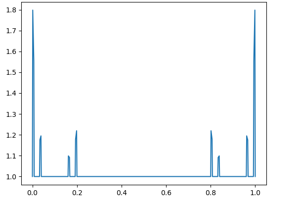
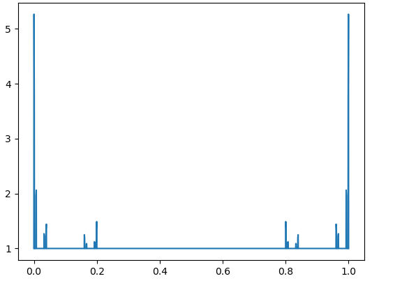
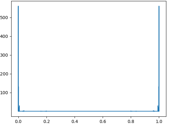
By [4, Theorem 4.4], in the case of small Cantor sets ($K^{\alpha }$ with $\alpha \ge 2$), the choice of $Y_{s-1}$ as the interpolating set provides a bounded subsequence of the Lebesgue constants. However, for “large” Cantor sets such as $K_{\beta }$, only one fundamental polynomial at a certain point takes sufficiently large values for large $s$.

We first consider the classical Cantor ternary set $K_{1/3}$. Table 1 illustrates the absolute values of fundamental Lagrange polynomials $l_{k,2^s}$ evaluated at the first node of the next level ${\mathrm{\ell }}_s$ for $1\le s\le 7$, $1\le k\le 2^s$. By comparison of these values to the graphs of the corresponding Lebesgue functions (Fig. 1), we observe that for each $s$, there exist a handful of polynomials that dominate rest of them and determine the behaviour of the Lebesgue constants. For $s\ge 3$, the values marked in red are the largest of their levels and they correspond to the value of the polynomial $l_{m,2^s}$, where $m\le 2^s$ is such that $x_m=\sum _{n=1}^s{(-1)}^{n+1}{\mathrm{\ell }}_n$. Explicitly, if $s$ is odd then $m=(2^s+1)/3$, if $s$ is even then $m=(2^s+2)/3$. Moreover, for these $s,m$, we have the ratios $5\le \left|\frac{{\lambda }_{2^s}({\mathrm{\ell }}_s)}{l_{m,2^s}({\mathrm{\ell }}_s)}\right|\le 6$, which exhibit the aforementioned similarity of behaviours.

On the other hand, comparing these results with the lower bounds corresponding to $|l_{k,2^s}({\mathrm{\ell }}_s)|$ for $k=2^{s-1}-1$ which were estimated in a more general setting in [4, Lemma 3.1], we see that the latter are quite rough.

For $s\in \mathbb{N}$, the fundamental polynomials $l_{k,2^s},k=1,2,..,2^s$ correspond to interpolating nodes $Y_{s-1}$. In Table 2, we evaluate maximal values of these polynomials over points of $Y_s$ and denote this by $M_{k,s}$. That is, we have $M_{k,s}={\max }_{x\in Y_s}|l_{k,2^s}(x)|.$

Comparing these values to the graphs of the Lebesgue functions of corresponding degree, it is evident that the fundamental polynomials that have comparable maxima with respect to the corresponding Lebesgue constant, attain their maximal values in either the first or the last interval of their level. These correspond to the polynomial $l_{m,2^s}$ (marked by red) and the ones corresponding to the adjacent nodes of $x_m$. In order to see this explicitly, one can also compare the values from Table 1 and Table 2 directly and notice for the aforementioned polynomials the agreement of values $M_{k,s}$ and the values at the first node of the next level.

	1	2	3	4	5	6	7	8	9	10	11	12	13	14	15	16
1	0,667	0,333
2	0,494	0,741	0,296	0,062
3	0,41	1,107	0,885	0,43	0,203	0,221	0,096	0,016
4	0,363	1,421	1,679	1,231	2,305	pink4,244	3,229	0,968	0,475	1,326	1,439	0,632	0,139	0,113	0,037	0,005

	1	2	3	4	5	6	7	8	9	10	11	12	13	14	15	16
5	0,335	1,672	2,532	2,387	9,753	23,5	23,51	9,308	72,26	283,5	pink435,2	272,8	183,2	221,7	107,8	20,04
6	0,317	1,863	3,318	3,683	24,7	70,3	83,17	38,99	1441	6755	12407	9315	10812	15741	9218	2065
7	0,306	2,001	3,97	4,91	45,57	144,6	190,8	99,75	9925	52003	1E+05	89595	1E+05	2E+05	2E+05	38918

	17	18	19	20	21	22	23	24	25	26	27	28	29	30	31	32
5	9,957	50,63	98,26	76,5	94,49	141,1	85,81	20,37	1,126	2,48	2,126	0,74	0,082	0,054	0,014	0,001
6	3E+05	2E+06	4E+06	4E+06	1E+07	pink2E+07	1E+07	4E+06	2E+06	6E+06	7E+06	3E+06	8E+05	7E+05	2E+05	30040
7	1E+08	8E+08	2E+09	2E+09	8E+09	2E+10	2E+10	5E+09	8E+09	3E+10	3E+10	2E+10	6E+09	6E+09	2E+09	3E+08

	33	34	35	36	37	38	39	40	41	42	43	44	45	46	47	48
6	14989	1E+05	3E+05	4E+05	1E+06	3E+06	3E+06	9E+05	1E+06	5E+06	6E+06	3E+06	1E+06	1E+06	5E+05	73047
7	1E+13	9E+13	3E+14	4E+14	2E+15	6E+15	6E+15	3E+15	2E+16	6E+16	pink9E+16	6E+16	3E+16	4E+16	2E+16	3E+15
	49	50	51	52	53	54	55	56	57	58	59	60	61	62	63	64
6	255,3	1092	1784	1170	868,5	1096	563,8	113,3	1,446	2,717	1,989	0,591	0,041	0,023	0,005	4E-04
7	1E+15	5E+15	1E+16	8E+15	1E+16	1E+16	9E+15	2E+15	1E+14	3E+14	3E+14	1E+14	1E+13	8E+12	2E+12	2E+11

	65	66	67	68	69	70	71	72	73	74	75	76	77	78	79	80
7	1E+11	1E+12	4E+12	6E+12	5E+13	1E+14	2E+14	7E+13	1E+15	4E+15	7E+15	4E+15	3E+15	4E+15	2E+15	4E+14
	81	82	83	84	85	86	87	88	89	90	91	92	93	94	95	96
7	1E+15	7E+15	1E+16	1E+16	2E+16	3E+16	2E+16	5E+15	8E+14	2E+15	2E+15	7E+14	1E+14	9E+13	3E+13	3E+12
	97	98	99	100	101	102	103	104	105	106	107	108	109	110	111	112
7	4E+07	3E+08	7E+08	7E+08	2E+09	4E+09	3E+09	9E+08	5E+08	1E+09	2E+09	8E+08	2E+08	2E+08	6E+07	9E+06
	113	114	115	116	117	118	119	120	121	122	123	124	125	126	127	128
7	1479	5671	8305	4885	2617	2963	1368	246,7	1,201	2,03	1,336	0,357	0,018	0,009	0,002	1E-04

Table 1. Values $|l_{k,2^s}({\mathrm{\ell }}_s)|$ for $1\le s\le 7$ and $k\le 2^s$.

	1	2	3	4	5	6	7	8	9	10	11	12	13	14	15	16
1	1	1
2	1	1,037	1,037	1
3	1	1,274	1	1	1	1,274	1
4	1	1,445	1,679	1,231	2,305	pink4,244	3,229	1	3,229	4,244	2,305	1,231	1,679	1,445		1
	1	2	3	4	5	6	7	8	9	10	11	12	13	14	15	16
5	1	1,672	2,532	2,387	9,753	23,5	23,51	9,308	72,26	283,5	pink435,2	272,8	183,2	221,7	107,8	20,04
6	1	1,863	3,318	3,683	24,7	70,3	83,17	38,99	1441	6755	12407	9315	10812	15741	9218	2065
7	1	2,001	3,97	4,91	45,57	144,6	190,8	99,75	9925	52003	1E+05	89595	1E+05	2E+05	2E+05	38918
	17	18	19	20	21	22	23	24	25	26	27	28	29	30	31	32
5	20,04	107,8	221,7	183,2	272,8	435,2	283,5	72,26	9,308	23,51	23,5	9,753	2,387	2,532	1,672	1
6	3E+05	2E+06	4E+06	4E+06	1E+07	pink2E+07	1E+07	4E+06	2E+06	6E+06	7E+06	3E+06	8E+05	7E+05	2E+05	30040
7	1E+08	8E+08	2E+09	2E+09	8E+09	2E+10	2E+10	5E+09	8E+09	3E+10	3E+10	2E+10	6E+09	6E+09	2E+09	3E+08

Table 2. Values $M_{k,s}$ for $1\le s\le 7$ and $k\le 2^s$.

	33	34	35	36	37	38	39	40	41	42	43	44	45	46	47	48
6	30040	2E+05	7E+05	8E+05	3E+06	7E+06	6E+06	2E+06	4E+06	1E+07	2E+07	1E+07	4E+06	4E+06	2E+06	3E+05
7	1E+13	9E+13	3E+14	4E+14	2E+15	6E+15	6E+15	3E+15	2E+16	6E+16	pink9E+16	6E+16	3E+16	4E+16	2E+16	3E+15
	49	50	51	52	53	54	55	56	57	58	59	60	61	62	63	64
6	2065	9218	15741	10812	9315	12407	6755	1441	38,99	83,17	70,3	24,7	3,683	3,318	1,863	1
7	1E+15	5E+15	1E+16	8E+15	1E+16	1E+16	9E+15	2E+15	1E+14	3E+14	3E+14	1E+14	1E+13	8E+12	2E+12	2E+11
	65	66	67	68	69	70	71	72	73	74	75	76	77	78	79	80
7	2E+11	2E+12	8E+12	1E+13	1E+14	3E+14	3E+14	1E+14	2E+15	9E+15	1E+16	1E+16	8E+15	1E+16	5E+15	1E+15
	81	82	83	84	85	86	87	88	89	90	91	92	93	94	95	96
7	3E+15	2E+16	4E+16	3E+16	6E+16	9E+16	6E+16	2E+16	3E+15	6E+15	6E+15	2E+15	4E+14	3E+14	9E+13	1E+13
	97	98	99	100	101	102	103	104	105	106	107	108	109	110	111	112
7	3E+08	2E+09	6E+09	6E+09	2E+10	3E+10	3E+10	8E+09	5E+09	2E+10	2E+10	8E+09	2E+09	2E+09	8E+08	1E+08
	113	114	115	116	117	118	119	120	121	122	123	124	125	126	127	128
7	38918	2E+05	2E+05	1E+05	89595	1E+05	52003	9925	99,75	190,8	144,6	45,57	4,91	3,97	2,001	1

Figure 1. $\beta =1/3$, ${\lambda }_{2^2}$ (left), ${\lambda }_{2^3}$ (right)

Figure 2. $\beta =1/3$, ${\lambda }_{2^4}$ (left), ${\lambda }_{2^5}$ (right)

Figure 3. $\beta =1/3$, ${\lambda }_{2^6}$ (left), ${\lambda }_{2^7}$ (right)

Fig. 1 – Fig. 3 give the graphs of ${\lambda }_{2^s}$, $2\le s\le 7$ for $K_{1/3}$. We observe fast growth of ${\mathrm{\Lambda }}_{2^s}(Y_{s-1},K_{1/3}).$

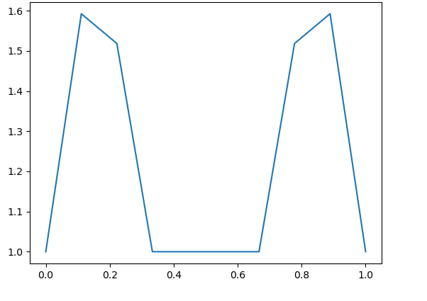
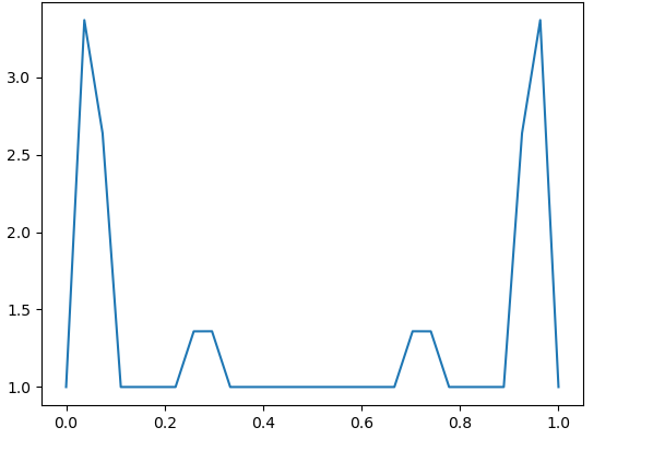
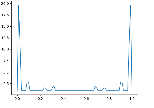
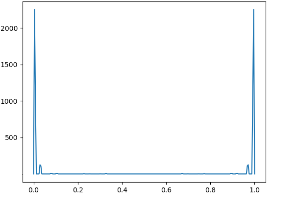
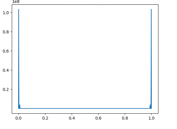
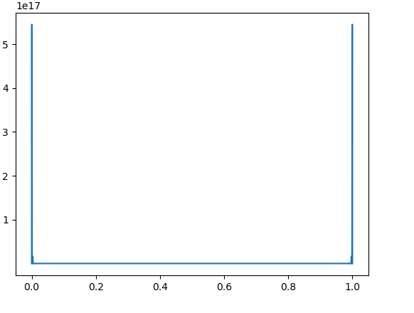
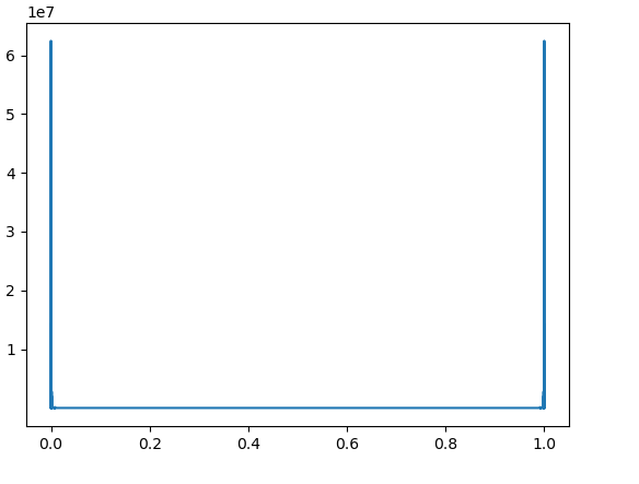
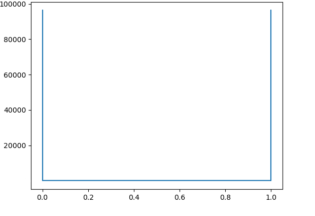
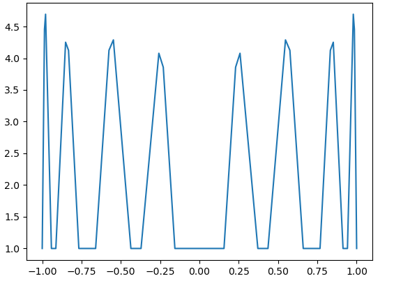
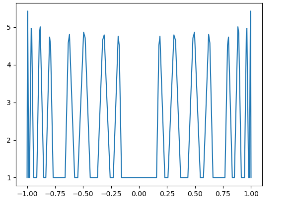
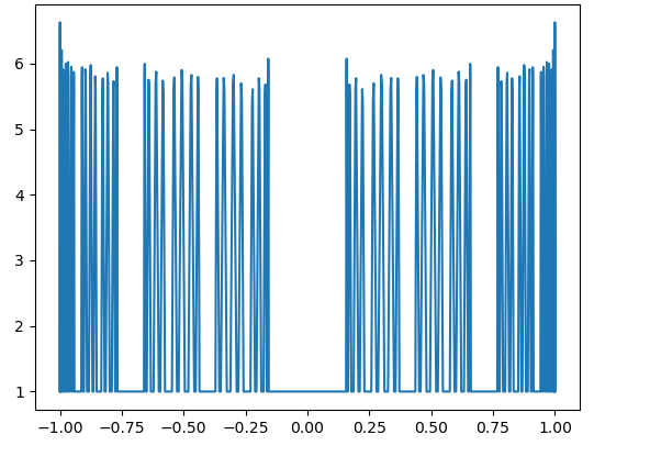
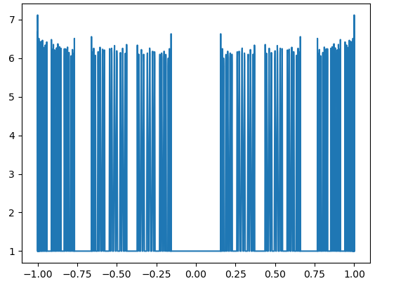
Numerical results demonstrate the exponential growth of these values, which correspond to in [4, Theorem 3.2]. Fig. 4 – Fig. 9 contain the graphs of ${\lambda }_{2^s},2\le s\le 8$ for $K_{\beta }$ with $\beta =1/5$ and $\beta =1/10.$

Figure 4. $\beta =1/5$, ${\lambda }_{2^2}$ (left), ${\lambda }_{2^3}$ (right)

Figure 5. $\beta =1/5$, ${\lambda }_{2^4}$ (left), ${\lambda }_{2^5}$ (right)

Figure 6. $\beta =1/5$, ${\lambda }_{2^6}$ (left), ${\lambda }_{2^7}$ (right)

Figure 7. $\beta =1/10$, ${\lambda }_{2^4}$ (left), ${\lambda }_{2^5}$ (right)

Figure 8. $\beta =1/10$, ${\lambda }_{2^6}$ (left), ${\lambda }_{2^7}$ (right)

Figure 9. $\beta =1/10$, ${\lambda }_{2^7}$ (left), ${\lambda }_{2^8}$ (right)

From these figures, we observe that the local maximum values ${\lambda }_{2^s}$ become smaller when $\beta$ decreases. However, even for small $\beta$ the figures illustrate a fast growth of ${\mathrm{\Lambda }}_{2^s}(Y_{s-1},K_{\beta }).$ Of course this does not support from [5, Theorem 6.2] (see [4, Section 3] for a more detailed discussion of this contradiction).

3. Lebesgue functions on $K^{\alpha }$

In the Cantor process corresponding to $K^{\alpha }$, the length of intervals converge to zero exponentially, whilist for $K_{\beta }$ it was geometrically. So in this sense the sets $K^{\alpha }$ are smaller than $K_{\beta }$. Based upon the previous results, we have the intuition that smaller sets correspond to smaller Lebesgue constants. The results from the numerical experiments for $K^{\alpha }$ support this intuition and illustrate numerically in [4, Corollary 4.5]: the sequence ${({\mathrm{\Lambda }}_{2^s}(Y_{s-1},K^{\alpha }))}_{s=1}^{\mathrm{\infty }}$ is bounded if and only if $\alpha \ge 2.$

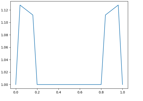
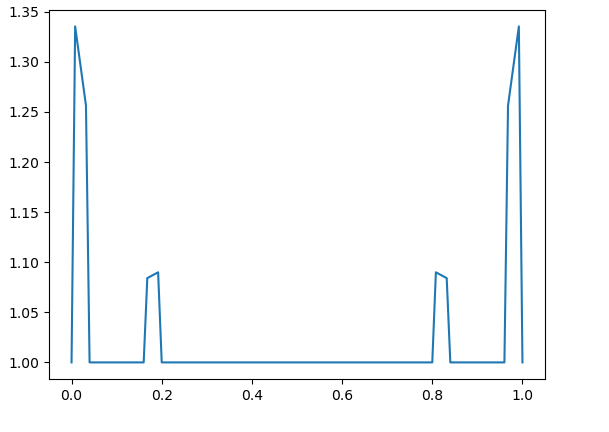
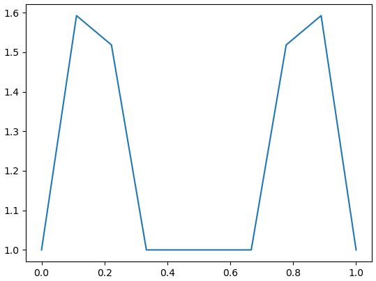
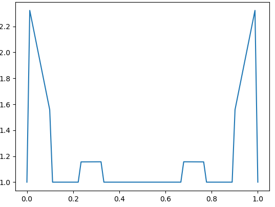
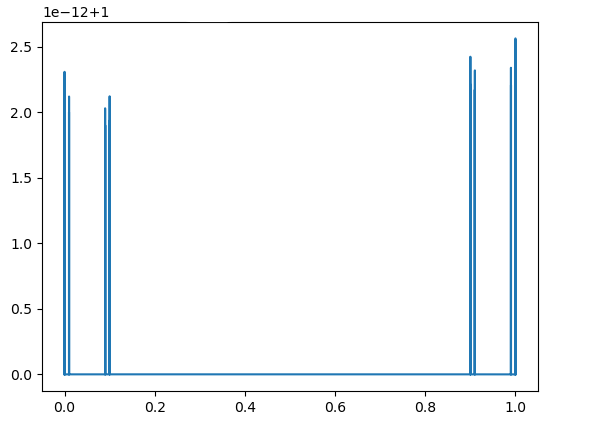
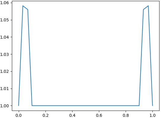
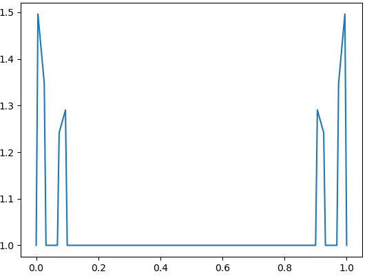
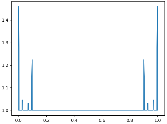
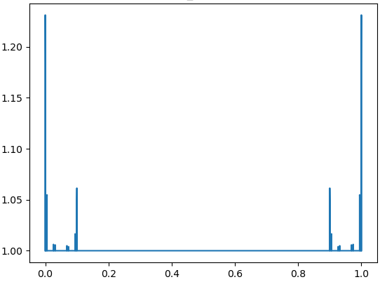
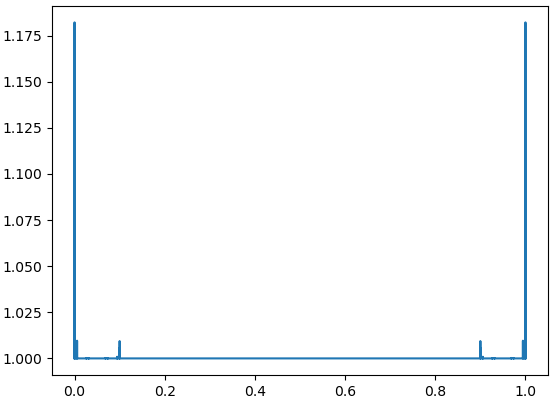
Fig. 10 – Fig. 13 contain the graphs of ${\lambda }_{2^s}$ for $K^2$ with ${\mathrm{\ell }}_1=1/3$ and ${\mathrm{\ell }}_1=1/10.$ We see that the local maxima of the Lebesgue functions decrease fast to one.

Figure 10. $\alpha =2$, ${\mathrm{\ell }}_1=1/3$, ${\lambda }_{2^2}$ (left), ${\lambda }_{2^3}$ (right)

Figure 11. $\alpha =2$, ${\mathrm{\ell }}_1=1/3$, ${\lambda }_{2^4}$ (left), ${\lambda }_{2^5}$ (right)

Figure 12. $\alpha =2$, ${\mathrm{\ell }}_1=1/10$, ${\lambda }_{2^2}$ (left), ${\lambda }_{2^3}$ (right)

Figure 13. $\alpha =2$, ${\mathrm{\ell }}_1=1/10$, ${\lambda }_{2^4}$ (left), ${\lambda }_{2^5}$ (right)

In general, we have a function of two variables $F_s({\mathrm{\ell }}_1,\alpha ):={\mathrm{\Lambda }}_{2^s}(Y_{s-1},K^{\alpha }({\mathrm{\ell }}_1)),$ where $\alpha >1$, ${\mathrm{\ell }}_1\le 1/3$ with

(1) $$3{\mathrm{\ell }}_1^{\alpha -1}\le 1.$$

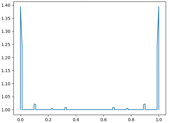
By [4, Theorem 4.4], the fixed values and ${\mathrm{\ell }}_1\le {\left(\frac{1}{3}\right)}^{\frac{1}{\alpha -1}}$ gives $F_s({\mathrm{\ell }}_1,\alpha )\to \mathrm{\infty }$ as $s\to \mathrm{\infty }.$ Following our intuition, in order to get fast growth of $F_s$ we have to take values of $\alpha$ close to 1 and not very small values of ${\mathrm{\ell }}_1$. However, by the restriction (1), this is impossible. We guess that for this reason and since our computational abilities are limited to values of $s\le 6$, the results from Fig. 14 – Fig. 16 do not show the growth of $F_s.$

Figure 14. $\alpha =1.5$, ${\mathrm{\ell }}_1=1/3$, ${\lambda }_{2^2}$ (left), ${\lambda }_{2^3}$ (right)

Figure 15. $\alpha =1.5$, ${\mathrm{\ell }}_1=1/3$, ${\lambda }_{2^4}$ (left), ${\lambda }_{2^5}$ (right)

Figure 16. $\alpha =1.5$, ${\mathrm{\ell }}_1=1/10$, ${\lambda }_{2^6}$

Let us note that $K^{\alpha }$ is polar if and only if $\alpha \ge 2$, see, e.g., in [6, Chapter V, §6, Theorem 3] or [1, Chapter IV, Theorem 3]. It gives immediately.

Proposition 1.

The sequence ${({\mathrm{\Lambda }}_{2^s}(Y_{s-1},K^{\alpha }))}_{s=1}^{\mathrm{\infty }}$ is bounded if and only if the set $K^{\alpha }$ is polar.

In the next section we will show that there are both polar and non-polar sets from the third family with a bounded sequence ${({\mathrm{\Lambda }}_{2^s}(Y_{s-1},K(\gamma )))}_{s=1}^{\mathrm{\infty }}.$ Now we present an example of a polar set $K^{({\alpha }_s)}$ for which the corresponding subsequence of Lebesgue constants is not bounded. It should be mentioned that Privalov constructed in [7] a polar set $K$ (in fact countable) such that for any array of interpolating nodes from $K$ the corresponding sequence of Lebesgue constants is not bounded, so $K$ is outside $ℬℒ𝒞$ in notations from [4].

Example 2.

Let ${\alpha }_k=2-2{\delta }_k$ and ${\pi }_s:={\prod }_{k=2}^s(1-{\delta }_k).$ If ${\pi }_s\to 0$ as $s\to \mathrm{\infty }$ with the divergent series ${\sum }_{s=2}^{\mathrm{\infty }}{\pi }_s,$ then the set $K^{({\alpha }_s)}$ is polar and ${\mathrm{\Lambda }}_{2^s}(Y_{s-1},K^{({\alpha }_s)})\to \mathrm{\infty }$ as $s\to \mathrm{\infty }.$

Indeed, by [1], the set $K^{({\alpha }_s)}$ is polar if and only if the series ${\sum }_{s=2}^{\mathrm{\infty }}\frac{{\alpha }_2{\alpha }_3\mathrm{\cdots }{\alpha }_s}{2^s}$ diverges. Hence, by the condition, $K^{({\alpha }_s)}$ is polar. On the other hand, by [4, Lemma 3.1],

$$|l_k({\mathrm{\ell }}_s)|\ge {\mathrm{\ell }}_s{\left(\frac{1-{\mathrm{\ell }}_s}{1-{\mathrm{\ell }}_1+{\mathrm{\ell }}_{s-1}}\right)}^{2^{s-1}},$$

where $k=2^{s-1}-1$ with $x_k={\mathrm{\ell }}_1-{\mathrm{\ell }}_{s-1}.$ Here, $s\ge 3,$ so ${\mathrm{\ell }}_1(1-{\mathrm{\ell }}_s)>{\mathrm{\ell }}_{s-1},$ which implies $\frac{1-{\mathrm{\ell }}_s}{1-{\mathrm{\ell }}_1+{\mathrm{\ell }}_{s-1}}>\frac{1}{1-{\mathrm{\ell }}_1}.$ Therefore,

$${\mathrm{\Lambda }}_{2^s}(Y_{s-1},K^{({\alpha }_s)})\ge |l_k({\mathrm{\ell }}_s)|\ge {\mathrm{\ell }}_1^{{\alpha }_2{\alpha }_3\mathrm{\cdots }{\alpha }_s}\cdot {\left(\frac{1}{1-{\mathrm{\ell }}_1}\right)}^{2^{s-1}}={\left(\frac{{\mathrm{\ell }}_1^{{\pi }_s}}{1-{\mathrm{\ell }}_1}\right)}^{2^{s-1}}.$$

For large enough $s,$ by the condition, ${\mathrm{\ell }}_1^{{\pi }_s}>1-{\mathrm{\ell }}_1.$ Hence, ${\mathrm{\Lambda }}_{2^s}(Y_{s-1},K^{({\alpha }_s)})\to \mathrm{\infty }$ as $s\to \mathrm{\infty }.$

4. Lebesgue functions on $K(\gamma )$

Finally, we turn our attention to the family of weakly-equilibrium sets $K(\gamma )$. Here each set is the intersection of the inverse polynomial images ${\left(\frac{2}{r_s}{P}_{2^s}+1\right)}^{-1}\left([-1,1]\right).$

By (3.1) in [3], the set $K(\gamma )$ is non-polar if and only if

(2)

[4, Theorem 6.3] gives boundedness of ${({\mathrm{\Lambda }}_{2^s}(Y_{s-1},K(\gamma )))}_{s=1}^{\mathrm{\infty }}$ provided ${\gamma }_s\le 1/32$ for $s\in \mathbb{N}$ and . It is easy to find sequences $\gamma$ satisfying these conditions with (2), as well as without it.

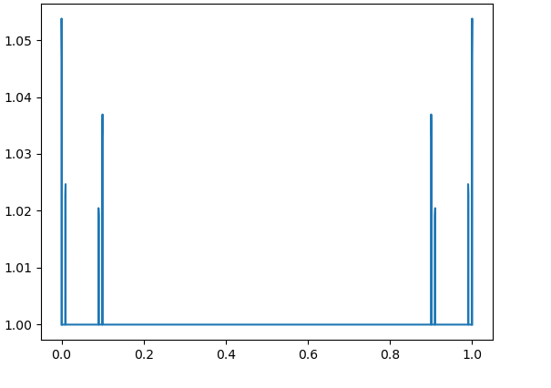
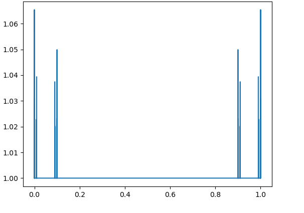
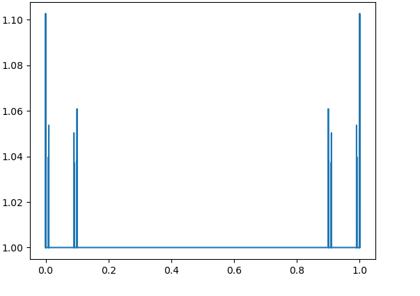
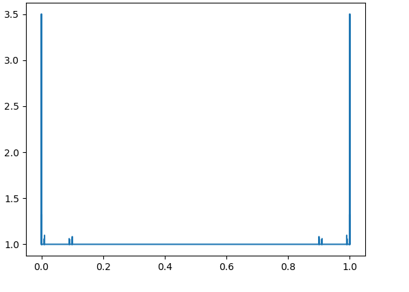
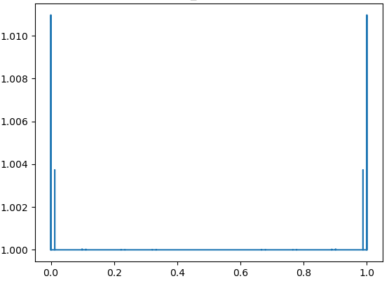
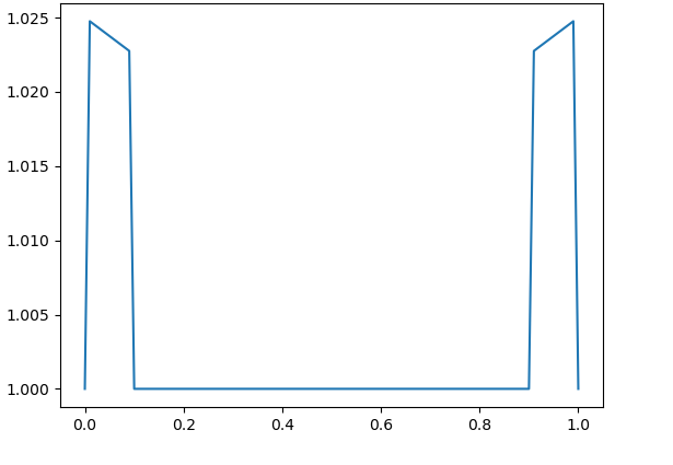
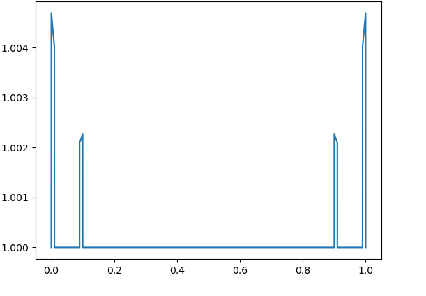
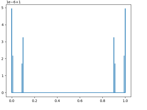
Here, in Fig. 17 – Fig. 20, we observe that even for the large values of the parameters (${\gamma }_s=0.24$ for all $s$), the magnitudes of ${\mathrm{\Lambda }}_{2^s}(Y_{s-1},K(\gamma ))$ are not large for $s\le 8.$

Figure 17. $\gamma \simeq 0.24$, ${\lambda }_{2^2}$ (left), ${\lambda }_{2^3}$ (right)

Figure 18. $\gamma \simeq 0.24$, ${\lambda }_{2^5}$ (left), ${\lambda }_{2^6}$ (right)

Figure 19. $\gamma \simeq 0.24$, ${\lambda }_{2^6}$ (left), ${\lambda }_{2^7}$ (right)

Figure 20. $\gamma \simeq 0.24$, ${\lambda }_{2^8}$

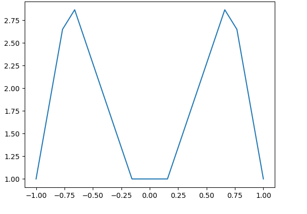
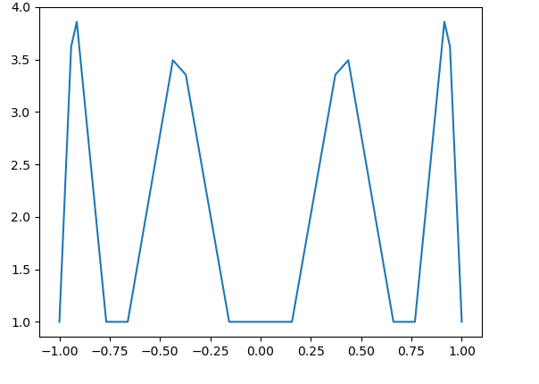
On the other hand, in the limit case, when ${\gamma }_s=1/4$ for all $s$, we have $K(\gamma )=[0,1],$ see [2, Example 1 from Section 4]. In this case, $Y_{s-1}$ consists of zeros of the Chebyshev polynomial $T_{2^s,[0,1]}$, corresponding to the interval $[0,1]$ with the logarithmic growth of the Lebesgue constants. The numerical evidence from Fig. 17 – Fig. 20 is quite consistent with the hypothesis about the logarithmic growth of ${\mathrm{\Lambda }}_{2^s}(Y_{s-1},K(\gamma ))$ for such values of the parameters. We guess that the condition is more important for the boundedness of ${({\mathrm{\Lambda }}_{2^s}(Y_{s-1},K(\gamma )))}_{s=1}^{\mathrm{\infty }}$ than the second restriction. Indeed, even in the case of arbitrary small ${\gamma }_0$, the condition ${\gamma }_s={\gamma }_0$ for all $s$ gives a uniformly perfect set $K(\gamma )$ ([2, Theorem 3]), which is more close in its nature to $K_{\beta }$ than to $K^{\alpha }$. Recall that the sequence ${({\mathrm{\Lambda }}_{2^s}(Y_{s-1},K_{\beta }))}_{s=1}^{\mathrm{\infty }}$ is not bounded for any $\beta$. For the definition of uniformly perfect sets, see, e.g., [2].

5. Conclusions

Based on numerical experiments as well as theoretical results from [4], we conclude that for Cantor-type sets $K$, the values ${\mathrm{\Lambda }}_{2^s}(Y_{s-1},K)$

1. are smaller for smaller sets,

2. may be bounded for sufficiently small $K$,

3. increase fast to infinity for symmetric uniformly perfect Cantor sets,

4. may be bounded even for non-polar sets, if $K$ is a “good” generalized Julia set constructed by means of a proper sequence of polynomials.

At the same time, the sequence ${({\mathrm{\Lambda }}_{2^s-1}(Z,K))}_{s=1}^{\mathrm{\infty }}$ is not bounded ([4, Theorems 4.6 and 6.4]) for any uniformly distributed set of nodes $Z$. What is more, by Theorem 6.4, even in the case of a “good” generalized Julia set, this sequence has a linear or faster growth.

Comparison of Corollary 4.5 and Theorem 4.6 allows us to assume that, at least for small Cantor-type sets, 5. uniform distribution of nodes is preferable.

Moreover, by [4, Theorem 5.1] we know that for $\alpha >2$ and for any distribution of nodes the Lebesgue Constants on $K^{\alpha }$ are unbounded, which gives $K^{\alpha }\notin ℬℒ𝒞$.

References

-
[1]
L. Carleson, Selected problems on exceptional sets, Toronto London Melbourne: D. Van Nostrand (151 pp.), 1967.
- [2] A. Goncharov,Weakly equilibrium Cantor-type sets. Potential Anal. 40 (2014), no. 2, pp. 143–161. https://doi.org/10.1007/s11118-013-9344-y
![[Uncaptioned image]](ext-link.png)
- [3] A. Goncharov and B. Hatinoğlu, Widom factors. Potential Anal. 42 (2015), no. 3, pp. 671–680. https://doi.org./10.1007/s11118-014-9452-3
- [4] A. Goncharov and Y. Paksoy, Lebesgue constants for Cantor sets, Exp. Math. (2024), pp. 1–11. https://doi.org/10.1080/10586458.2024.2381676
[5]
S. N. Mergelyan, Certain questions of the constructive theory of functions (in Russian),
Trudy Matematicheskogo Instituta imeni VA Steklova 37 (1951), pp. 3–91.
- [6] R. Nevanlinna, Analytic functions, Springer-Verlag, New York-Berlin, 1970 viii+373 pp. https://doi.org/10.1007/978-3-642-85590-0
- [7] A.A. Privalov, Interpolation on countable sets (in Russian), Uspekhi Mat. Nauk 19 (1964), no. 4, pp. 197–200.