A numerical approach for
singularly perturbed parabolic reaction-diffusion
problem on a modified graded mesh

Abstract.

This paper addresses the numerical approximations of solutions for one dimensional parabolic singularly perturbed problems of reaction-diffusion type. The solution of this class of problems exhibit boundary layers on both sides of the domain. The proposed numerical method involves combining the backward Euler method on a uniform mesh for temporal discretization and an upwind finite difference scheme for spatial discretization on a modified graded mesh. The numerical solutions presented here are calculated using a modified graded mesh and the error bounds are rigorously assessed within the discrete maximum norm. The primary focus of this study is to underscore the crucial importance of utilizing a modified graded mesh to enhance the order of convergence in numerical solutions. The method demonstrates uniform convergence, with first-order accuracy in time and nearly second-order accuracy in space concerning the perturbation parameter. Theoretical findings are supported by numerical results presented in the paper.

1. Introduction

Singular perturbation problem consists of small parameter associated with highest oredr derivative in the equation. Presence of the parameter will cause the distortion in the solution in the vicinity of the boundary. Such problems have boundary or interior layers in their solutions. The interior layer develops when there is a discontinuity in the provided data, and the boundary layer happens when a term containing the highest order derivative is multiplied by a singular perturbation parameter. Furthermore, the problem is stiff due to the simultaneous presence of a discontinuous coefficient and a delay parameter, and the solution shows multi-scale character as $\epsilon \to 0$. Many physical and real world problems are followed by singularly perturbed parabolic problem. In [7], its applications to many field of interests have been described. One can refer the book [2] for the application of the problem in medicine while, [11, 13] are dealing with the applications of such problems in mechanics. There are many articles in the literature that are imerged as a result of convergence of numerical schemes applied to singularly perturbed problem of parabolic type, e.g., one can refer to the articles [7, 3, 4, 5].

Finite difference method (FDM) is a sort of numerical technique that approximates the derivatives in a differential equation by replacing them with finite differences, calculated over a discrete grid of points, to solve for the unknown function or solution. There are a lots of beauties of this methods including

• Discretization: FDM discretizes the continuous domain into a grid of points, allowing for numerical approximation.

• Approximation of derivatives: FDM approximates derivatives using finite differences, such as forward, backward, or central differences.

• Local accuracy: FDM has high local accuracy, meaning it’s accurate in small neighbourhood around each grid point.

• Global convergence: FDM can converge to the exact solution as the grid size decreases.

• Easy to implement: FDM is relatively simple to understand and implement, especially for simple geometries.

• Computational efficiency: FDM can be computationally efficient, especially for large-scale problems.

• Flexibility: FDM can be applied to various types of differential equations, including non-linear and time-dependent equations.

However, certain limitations to the method are grid dependence, numerical diffusion and boundary treatment. Overall, the finite difference method is a powerful tool for solving differential equations, offering a good balance between accuracy, efficiency, and simplicity.

The manuscripts that are utilizing the methods to obtain accuracy of discrtized solution include [10, 15, 18, 6]. Different variants of FDMs have been utilized to get the accuracy and convergence of the problem with different conditions and restrictions. [8] is the study of convection–reaction problem in which space direction is discretized by Shishkin mesh while Crank-Nikolson is adapted to discrtize in time direction. As a result, second order convergence in time domain and higher order convergence in space domain are gained, respectively. except this [9] is the study of the discrtization of convection-reaction problem using Euler technique in time domain and a central difference method comprises with space domain. Almost second order convergence upto logarithmic term is shown as a convergence result.

Throughing these manuscripts, we have considered the singularly perturbed parabolic initial-boundary-value problem (IBVP):

(1)

where,

(2) $${𝔏}_{\epsilon }u\equiv -\epsilon u_{rr}+b(r)u$$

is a small parameter, $b$ and $f$ are sufficiently smooth functions with $b(r)\ge \delta >0$ for $r\in {\overline{\mathrm{{\rm Y}}}}_r=[0,1]$. Here, $\mathrm{\Pi }$ = ${\mathrm{{\rm Y}}}_r\times {\mathrm{{\rm Y}}}_{\theta }$, where ${\mathrm{{\rm Y}}}_r=(0,1)$ and ${\mathrm{{\rm Y}}}_{\theta }=(0,𝒯]$ and also $\mathrm{\Lambda }={\mathrm{\Lambda }}_{l^{\ast }}\cup {\mathrm{\Lambda }}_b\cup {\mathrm{\Lambda }}_{r^{\ast }}.$ The above considered singular perturbation parameter is $\epsilon \in (0,1]$ and also considered function $b(r)$, $f(r,\theta )$, ${\psi }_b(r)$, ${\psi }_l^{\ast }(\theta )$ and ${\psi }_r^{\ast }(\theta )$ are sufficiently smooth, bounded and also satisfy the condition $b(r)\ge 0.$ The reduced problem corresponding to $(\text{<a href="\#S1.E1" title="Equation 1 ‣ 1. Introduction ‣ A numerical approach for singularly perturbed parabolic reaction-diffusion problem on a modified graded mesh" class="ltx\_ref ltx\_font\_italic"><span class="ltx\_text ltx\_ref\_tag">1</span></a>})$ is

(3) $$\{\begin{array}{cc}\frac{\partial u(r,\theta )}{\partial \theta }+b(r)u(r,\theta )=f(r,\theta ),\forall (r,\theta )\in \mathrm{\Pi },\hfill & \\ u(r,\theta )={\psi }_b(r),r\in {\mathrm{\Lambda }}_b.\hfill & \end{array}$$

As $(\text{<a href="\#S1.E1" title="Equation 1 ‣ 1. Introduction ‣ A numerical approach for singularly perturbed parabolic reaction-diffusion problem on a modified graded mesh" class="ltx\_ref ltx\_font\_italic"><span class="ltx\_text ltx\_ref\_tag">1</span></a>}$) is characterized by boundary layers, uniform meshes do not work properly [1], which results to the construction of non-uniform and layer adapted meshes. In recent days, layer adapted meshes are better in handling the problems possess boundary and interior layers. [3, 14, 17] are the study about the convergence of finite difference methods over Shishkin mesh and other layer adapted meshes for reaction-convection equations.

In the present study, we have adopted the modified graded mesh for spatial domain. simple upwinding are introduced for discretizing the problem and uniform grid is taken place as domain discretization in time domain. As a consequence, almost second order convergence upto logarithimic factor we have achieved in spactial direction as a convergence rate of numerical solution which is optimal. Finally, we have presented two test problems to validate our theretical conclusions.

The rest of the manuscripts are adored in the following manner: Section 2 is a brief study of the analytical behavior of the problem, including an introduction to the appropriate Hölder spaces. The discussion includes the maximum principle for the differential operator, highlighting its role in ensuring $\epsilon$-uniform stability. We also present sufficient compatibility conditions on the initial and boundary data to ensure the existence, uniqueness, and appropriate regularity of the problem’s solutions. In Theorem 2, both classical and new sharper $\epsilon$-uniform bounds in the maximum norm on the derivative of the solution are discussed. The latter are obtained by means of a new decomposition of the solution, which leads to a deceptively simple proof of the required results. We generated the modified graded mesh and their properties are contained in Section 3. The upwind finite difference scheme is constructed in Section 4. We have completed error analysis for the presented method in Section 5. In Section 6, the numerical results are reported, which validate the results predicted by the theory and in fact show that the numerical methods work equally well in practice for a much broader class of problems than the theory predicts. Section 7 ends with the conclusion.

Notation: $𝒞$ is used as a generic constant throughout the paper and also, $𝒞$ is independent of the perturbation parameter $\epsilon$ and the mesh point $𝒩$ and we use discrete maximum norm to study convergence which is defined as,

$${\Vert u\Vert }_{\mathrm{\Pi }}=\underset{r\in \mathrm{\Pi }}{\max }|u(r)|.$$

2. Analytical behaviour of the continuous problem

To explore the consistency of solutions to the time-dependent problem under consideration, we introduce certain function spaces characterized by Hölder continuity in both spatial and temporal dimensions. Specifically, consider $\mathrm{{\rm Y}}\subset ℝ$ and $\mathrm{\Pi }$ be a convex domain in $\overline{\mathrm{{\rm Y}}}\times [0,T].$ Again we suppose that $\kappa \in ℝ$ and fulfilled the condition Then a function $y$ is said to be Hölder continuous in $\mathrm{\Pi }$ of degree $\kappa$ if, for all $(r,\theta ),(r^{\prime },{\theta }^{\prime })\in \mathrm{\Pi },$

$$|u(r,\theta )-u(r^{\prime },{\theta }^{\prime })|\le 𝒞{\left({|r-r^{\prime }|}^2+|\theta -{\theta }^{\prime }|\right)}^{\kappa /2}.$$

Notice the distinction in the metrics employed for the spatial and temporal variables. The collection of all Holder continuous functions constitutes a normed linear vector space denoted by ${𝒞}_{\kappa }^0(\mathrm{\Pi })$, equipped with the norm

$${\Vert u\Vert }_{\kappa ,\mathrm{\Pi }}={\Vert u\Vert }_{\mathrm{\Pi }}+\underset{(r,\theta ),(r^{\prime },{\theta }^{\prime })\in \mathrm{\Pi }}{sup}\frac{|u(r,\theta )-u(r^{\prime },{\theta }^{\prime })|}{{({|r-r^{\prime }|}^2+|\theta -{\theta }^{\prime }|)}^{\kappa }/2},$$

where

$${\Vert u\Vert }_{\mathrm{\Pi }}=\underset{(r,\theta )\in \mathrm{\Pi }}{sup}|u(r,\theta )|.$$

We introduce the subspace ${𝒞}_{\kappa }^p(\mathrm{\Pi })$ of ${𝒞}_{\kappa }^0(\mathrm{\Pi })$ for each integer $p\ge 1$. These are functions within ${𝒞}_{\kappa }^0(\mathrm{\Pi })$ that possess Hölder continuous derivatives. and also introduced

$${𝒞}_{\kappa }^p(\mathrm{\Pi })=\{u:\frac{{\partial }^{i+j}u}{\partial r^i\partial {\theta }^j}\in {𝒞}_{\kappa }^0(\mathrm{\Pi })\text{for all positive integers i and j with }0\le i+2j\le p\}.$$

The norm on ${𝒞}_{\kappa }^p(\mathrm{\Pi })$ is taken to be

$${\Vert u\Vert }_{p,\kappa ,\mathrm{\Pi }}=\underset{0\le i+2j\le p}{\max }{\Vert \frac{{\partial }^{i+j}u}{\partial r^i\partial {\theta }^j}\Vert }_{\kappa ,\mathrm{\Pi }}.$$

Observe once more the distinct handling of space and time derivatives. For $u\in {𝒞}_{\kappa }^p(\mathrm{\Pi })$ and $0\le q\le p$, we also define the following semi-norms:

$${\Vert u\Vert }_{q,\kappa ,\mathrm{\Pi }}=\underset{i+2j\le q}{\max }{\Vert \frac{{\partial }^{i+j}u}{\partial r^i\partial {\theta }^j}\Vert }_{\kappa ,\mathrm{\Pi }}.$$

From these definitions, it is clear that

$${\Vert u\Vert }_{p,\kappa ,\mathrm{\Pi }}=\underset{0\le q\le p}{\max }{\Vert u\Vert }_{q,\kappa ,\mathrm{\Pi }}$$

Adopting the notational convention ${\Vert u\Vert }_{0,\kappa ,\mathrm{\Pi }}={|u|}_{0,\kappa ,\mathrm{\Pi }}={\Vert u\Vert }_{\kappa ,\mathrm{\Pi }}$, when the domain is apparent or of no specific importance, $\mathrm{\Pi }$ is typically omitted.

Furthermore, the initial functions ${\psi }_b(r)$, are essential to meet compatibility conditions at corner points of the domain, namely at $(0,0)$ and $(1,0)$. These points significantly represents the boundaries or changes in the boundary conditions, satisfying compatibility conditions at these points ensures a consistency where the boundary or initial conditions may change sharply. The required compatibility conditions at the corners are stated below,

${\psi }_b(0)$ $={\psi }_{l^{\ast }}(0),$

${\psi }_b(1)$ $={\psi }_{r^{\ast }}(0),$

$\frac{d{\psi }_{l^{\ast }}(0)}{d\theta }-\epsilon \frac{d^2{\psi }_b(0)}{d{r}^2}+b(0){\psi }_b(0)$ $=f(0,0),$

$\frac{d{\psi }_{r^{\ast }}(0)}{d\theta }-\epsilon \frac{d^2{\psi }_b(1)}{d{r}^2}+b(1){\psi }_b(1)$ $=f(1,0).$

Under the above compatibility condition, $(\text{<a href="\#S1.E1" title="Equation 1 ‣ 1. Introduction ‣ A numerical approach for singularly perturbed parabolic reaction-diffusion problem on a modified graded mesh" class="ltx\_ref ltx\_font\_italic"><span class="ltx\_text ltx\_ref\_tag">1</span></a>})$ possess unique solution with possibility of layer at both the end points $r=0$ and $r=1$.

Minimum Principle. Assume that $b\in {𝒞}^0(\overline{\mathrm{\Pi }})$ and let $\psi \in {𝒞}^2(\mathrm{\Pi })\cap {𝒞}^0(\overline{\mathrm{\Pi }})$ also suppose that $\psi \ge 0$ on $\mathrm{\Lambda }$ then ${𝔏}_{\epsilon }\psi \ge 0$ in $\mathrm{\Pi }$ implies that $\psi \ge 0$ in $\overline{\mathrm{\Pi }}.$

Proof.

Let us assume that for all $(r,\theta )\in \mathrm{\Lambda }$, we have $\psi (r,\theta )\ge 0$, and for all $(r,\theta )\in \mathrm{\Lambda }$, ${𝔏}_{\epsilon }\psi (r,\theta )\ge 0$. Now, we apply the differential operator ${𝔏}_{\epsilon }$ on $\psi$. To contradict we assume that there exists a point $(r_0,{\theta }_0)\in \mathrm{\Pi }$ such that , and $\psi (r_0,{\theta }_0)$ is a minimum of $\psi$ in $\mathrm{\Pi }$. Since, we have assumed that $\psi (r_0,{\theta }_0)$ minimum and also $\psi$ is differentiable, then by applying a second order differential operator ${𝔏}_{\epsilon }$, on $\psi$ shows that it has upward concavity, which contradicts our supposition that . Also, if $\psi$ attain its minimum on $\overline{\mathrm{\Pi }}$, then by assumption that $\psi (r,\theta )\ge 0$ for all $(r,\theta )\in \mathrm{\Pi }$ and hence on $\overline{\mathrm{\Pi }}$, $\psi$ must also be non-negative. ∎

Ensuring the stability of ${𝔏}_{\epsilon }$ and establishing an $\epsilon$-uniform bound for the solution $(\text{<a href="\#S1.E1" title="Equation 1 ‣ 1. Introduction ‣ A numerical approach for singularly perturbed parabolic reaction-diffusion problem on a modified graded mesh" class="ltx\_ref ltx\_font\_italic"><span class="ltx\_text ltx\_ref\_tag">1</span></a>})$ in the maximum norm naturally follows from this.

Theorem 1.

Consider any function $𝒮$ within the domain of the differential operator ${𝔏}_{\epsilon }$ in $(\text{<a href="\#S1.E1" title="Equation 1 ‣ 1. Introduction ‣ A numerical approach for singularly perturbed parabolic reaction-diffusion problem on a modified graded mesh" class="ltx\_ref"><span class="ltx\_text ltx\_ref\_tag">1</span></a>})$. Then

$$\Vert 𝒮\Vert \le (1+\alpha 𝒯)\max \{\Vert {𝔏}_{\epsilon }𝒮\Vert ,{\Vert 𝒮\Vert }_{\mathrm{\Lambda }}\},$$

and any solution $u(r,\theta )$ of $(\text{<a href="\#S1.E1" title="Equation 1 ‣ 1. Introduction ‣ A numerical approach for singularly perturbed parabolic reaction-diffusion problem on a modified graded mesh" class="ltx\_ref"><span class="ltx\_text ltx\_ref\_tag">1</span></a>})$ has the $\epsilon$-uniform upper bound

$$\Vert u(r,\theta )\Vert \le (1+\alpha 𝒯)\max \{\Vert f\Vert ,\Vert \phi \Vert \},$$

where $\alpha ={\max }_{\overline{\mathrm{\Pi }}}\{0,(1-b)\}\le 1/\delta .$

The subsequent classical theorem provides adequate conditions for guaranteeing the existence of a unique solution.

Theorem 2.

Suppose that $\phi =0,$ the data $b$ and $f$ $\in {𝒞}_{\lambda }^0(\overline{\mathrm{\Pi }}),$ and that the compatibility conditions

$$f(0,0)=f(1,0)=0$$

are fulfilled. then $(\text{<a href="\#S1.E1" title="Equation 1 ‣ 1. Introduction ‣ A numerical approach for singularly perturbed parabolic reaction-diffusion problem on a modified graded mesh" class="ltx\_ref"><span class="ltx\_text ltx\_ref\_tag">1</span></a>})$ has a unique solution $u$ and $u\in {𝒞}_{\lambda }^2(\overline{\mathrm{\Pi }}).$

sectionBounds on the solution and its derivatives

The proposed method’s error estimate, discussed below, is validated assuming that the solution of $(\text{<a href="\#S1.E1" title="Equation 1 ‣ 1. Introduction ‣ A numerical approach for singularly perturbed parabolic reaction-diffusion problem on a modified graded mesh" class="ltx\_ref ltx\_font\_italic"><span class="ltx\_text ltx\_ref\_tag">1</span></a>})$ exhibits a higher level of regularity than guaranteed by Theorem 4. Achieving this heightened regularity necessitates the imposition of stronger compatibility conditions at the two corners of $\overline{\mathrm{\Pi }}$. The additional compatibility conditions are

(4) $$\left(\frac{\partial }{\partial \theta }+\epsilon \frac{{\partial }^2}{\partial r^2}\right)\left(f\right)(0,0)=0\text{and}\left(\frac{\partial }{\partial \theta }+\epsilon \frac{{\partial }^2}{\partial r^2}\right)\left(f\right)(1,0)=0$$

Note that these conditions necessitate additional smoothness of $f$. The subsequent theorem establishes the existence of a smooth solution for the problem with homogeneous boundary conditions.

Theorem 3.

Assume that $\phi =0,$ the data $b$ and $f\in {𝒞}_{\lambda }^2(\mathrm{\Pi }),$ and that the compatibility conditions

$$f(0,0)=f(1,0)=0$$

and

$$\left(\frac{\partial }{\partial \theta }+\epsilon \frac{{\partial }^2}{\partial r^2}\right)\left(f\right)(0,0)=\left(\frac{\partial }{\partial \theta }+\epsilon \frac{{\partial }^2}{\partial r^2}\right)\left(f\right)(1,0)=0$$

are fulfilled. Then $(\text{<a href="\#S1.E1" title="Equation 1 ‣ 1. Introduction ‣ A numerical approach for singularly perturbed parabolic reaction-diffusion problem on a modified graded mesh" class="ltx\_ref"><span class="ltx\_text ltx\_ref\_tag">1</span></a>})$ has a unique solution $u$ and $u\in {𝒞}_{\lambda }^4(\mathrm{\Pi }).$ Furthermore, the derivatives of the solution $u$ satisfy, for all non-negative integers $i,j,$ such that $0\le i+2j\le 4,$

$${\Vert \frac{{\partial }^{i+j}{u}_{\epsilon }}{\partial r^i\partial {\theta }^j}\Vert }_{\mathrm{\Pi }}\le 𝒞{\epsilon }^{-i/2},$$

where the constant $𝒞$ is independent of $\epsilon .$

Proof.

The first part’s proof is provided in [12]. Bounds on the derivatives are acquired through the following process: by transforming the variable $r$ into the stretched variable $\tilde{r}=r/\sqrt{\epsilon }$, problem $(\text{<a href="\#S1.E1" title="Equation 1 ‣ 1. Introduction ‣ A numerical approach for singularly perturbed parabolic reaction-diffusion problem on a modified graded mesh" class="ltx\_ref ltx\_font\_italic"><span class="ltx\_text ltx\_ref\_tag">1</span></a>})$ becomes problem

(5) $\{\begin{array}{cc}-\frac{{\partial }^2\tilde{u}}{\partial {\tilde{r}}^2}+\tilde{b}\tilde{u}+\frac{\partial \tilde{u}}{\partial \theta }=\tilde{f}\text{on}{\tilde{\mathrm{\Pi }}}_{\epsilon }\hfill & \\ \tilde{u}=0,\hfill & \end{array}$

where ${\tilde{\mathrm{\Pi }}}_{\epsilon }=(0,1/\sqrt{\epsilon })\times (0,𝒯]$. The differential equation in $(\text{<a href="\#S2.E5" title="Equation 5 ‣ 2. Analytical behaviour of the continuous problem ‣ A numerical approach for singularly perturbed parabolic reaction-diffusion problem on a modified graded mesh" class="ltx\_ref ltx\_font\_italic"><span class="ltx\_text ltx\_ref\_tag">5</span></a>})$ is not dependent on $\epsilon .$ Utilizing the estimate (10.5) from [12], it is deduced that for all non-negative integers $i,j$ such that $0\le i+2j\le 4$, and all ${\widetilde{𝒩}}_{\delta }$ in ${\tilde{\mathrm{\Pi }}}_{\epsilon }$,

$${\Vert \frac{{\partial }^{i+j}\tilde{u}}{\partial {\tilde{r}}^i\partial {\theta }^j}\Vert }_{{\widetilde{𝒩}}_{\delta }}\le 𝒞(1+{\Vert \tilde{u}\Vert }_{{\widetilde{𝒩}}_{2\delta }}).$$

Hence, we used the Theorem 1 which bound on the $u_{\epsilon }$. ∎

The limits on the derivatives of the solution, as provided in Theorem 3, were initially deduced from classical findings. Nevertheless, it has been discovered that they lack sufficiency for proving the $\epsilon$-uniform error estimate. To address this, more robust boundaries on these derivatives are acquired through a methodology initially presented in [16]. A pivotal maneuver involves breaking down the solution,$u_{\epsilon }$, into components of smoothness and singularity.

Suppose that the solution $u$ of equation $(\text{<a href="\#S1.E1" title="Equation 1 ‣ 1. Introduction ‣ A numerical approach for singularly perturbed parabolic reaction-diffusion problem on a modified graded mesh" class="ltx\_ref ltx\_font\_italic"><span class="ltx\_text ltx\_ref\_tag">1</span></a>})$ and write in the form as

(6) $$u_{\epsilon }={ℛ}_{\epsilon }+{𝒮}_{\epsilon },$$

where ${ℛ}_{\epsilon }$ and ${𝒮}_{\epsilon }$ are smooth and singular components of $u_{\epsilon }$ .

Now, again decomposed the smooth component ${ℛ}_{\epsilon }$ in the form such that

$${ℛ}_{\epsilon }={ℛ}_0+\epsilon {ℛ}_1,$$

where the define the component ${ℛ}_0$ and ${ℛ}_1$ in the form as

$$b{ℛ}_0+\frac{\partial {ℛ}_0}{\partial \theta }=f\text{in}\mathrm{\Pi },{ℛ}_0=0\text{on}{\overline{\mathrm{\Lambda }}}_b,$$

$${𝔏}_{\epsilon }{ℛ}_1=\frac{{\partial }^2{ℛ}_0}{\partial r^2}\text{in}\mathrm{\Pi },{ℛ}_1=0\text{on}\mathrm{\Lambda }.$$

Therefore, it is evident that ${ℛ}_0$ represents the solution to the reduced problem and moreover, ${ℛ}_{\epsilon }$ satisfies

$${𝔏}_{\epsilon }{ℛ}_{\epsilon }=f\text{and}{ℛ}_{\epsilon }={ℛ}_0\text{on}{\mathrm{\Lambda }}_{l^{\ast }}\cup {\mathrm{\Lambda }}_{r^{\ast }}.$$

With ${ℛ}_{\epsilon }$ defined in this manner, it follows that ${𝒮}_{\epsilon }$ is determined and satisfies

$${𝔏}_{\epsilon }{𝒮}_{\epsilon }=0\text{in}\mathrm{\Pi }{𝒮}_{\epsilon }=0\text{on}\mathrm{\Pi }\text{and}{𝒮}_{\epsilon }=-{ℛ}_0\text{on}\overline{\mathrm{\Pi }}.$$

Now, we can also easily to write of ${𝒮}_{\epsilon }$ such that

$${𝒮}_{\epsilon }={𝒮}_l+{𝒮}_r,$$

where ${𝒮}_l$ and ${𝒮}_r$ are define by

$$\{\begin{array}{cc}{𝔏}_{\epsilon }{𝒮}_l=0\text{in}\mathrm{\Pi },\hfill & \\ {𝔏}_{\epsilon }{𝒮}_r=0\text{in}\mathrm{\Pi }\hfill & \end{array}$$

$$\{\begin{array}{cc}{𝒮}_l=-{ℛ}_0\text{on}{\mathrm{\Lambda }}_{l^{\ast }},\hfill & \\ {𝒮}_r=-{ℛ}_0\text{on}{\mathrm{\Lambda }}_{r^{\ast }},\hfill & \end{array}$$

$$\{\begin{array}{cc}{𝒮}_l=0\text{on}{\mathrm{\Lambda }}_b\cup {\mathrm{\Lambda }}_{r^{\ast }},\hfill & \\ {𝒮}_r=0\text{on}{\mathrm{\Lambda }}_{l^{\ast }}\cup {\mathrm{\Lambda }}_b\hfill & \end{array}$$

It’s evident that ${𝒮}_l$ and ${𝒮}_r$ denote the boundary layers on ${\mathrm{\Lambda }}_{l^{\ast }}$ and ${\mathrm{\Lambda }}_{r^{\ast }}$ , respectively. The theorem following contains the necessary non-classical bounds on ${ℛ}_{\epsilon }$ and ${𝒮}_{\epsilon }$, along with their derivatives.

Theorem 4.

Let’s consider problem $(\text{<a href="\#S1.E1" title="Equation 1 ‣ 1. Introduction ‣ A numerical approach for singularly perturbed parabolic reaction-diffusion problem on a modified graded mesh" class="ltx\_ref"><span class="ltx\_text ltx\_ref\_tag">1</span></a>})$. We assume that the data $b\in {𝒞}_{\lambda }^2(\overline{\mathrm{\Pi }})$ and $f\in {𝒞}_{\lambda }^4(\overline{\mathrm{\Pi }})$, and that the compatibility conditions of the previous theorem are met. Under these conditions, the reduced solution ${ℛ}_0$ exists and belongs to ${𝒞}_{\lambda }^4(\overline{\mathrm{\Pi }})$. Additionally, if the supplementary compatibility conditions are satisfied, then

(7) $$\frac{{\partial }^{2}f(0,0)}{\partial r^2}=\frac{{\partial }^{2}f(1,0)}{\partial r^2}=0$$

and

(8) $$\frac{\partial f(0,0)}{\partial \theta }=\frac{\partial f(1,0)}{\partial \theta }=0$$

are satisfied then ${ℛ}_1$ and ${𝒮}_{\epsilon }$ exists and ${ℛ}_1,{𝒮}_{\epsilon }\in {𝒞}_{\lambda }^4(\overline{\mathrm{\Pi }})$. Also, for all positive integers $i,j,$ such that $0\le i+2j\le 4$

$${\Vert \frac{{\partial }^{i+j}{ℛ}_{\epsilon }}{\partial r^i\partial {\theta }^j}\Vert }_{\overline{\mathrm{\Pi }}}\le 𝒞(1+{\epsilon }^{1-i/2}),$$

and for all $(r,\theta )\in \mathrm{\Pi }$,

$$\Vert \frac{{\partial }^{i+j}{𝒮}_l(r,\theta )}{\partial r^i\partial {\theta }^j}\Vert \le 𝒞{\epsilon }^{-i/2}{\text{e}}^{-r/\sqrt{\epsilon }}$$

and

$$\Vert \frac{{\partial }^{i+j}{ℛ}_r(r,\theta )}{\partial r^i\partial {\theta }^j}\Vert \le 𝒞{\epsilon }^{-i/2}{\text{e}}^{-(1-r)/\sqrt{\epsilon }},$$

where $𝒞$ is a constant independent of $\epsilon .$

Proof.

References for the existence and regularity results can be found in [12]. The proofs of the bounds on the functions and their derivatives are presented subsequently.

The reduced solution, denoted as ${ℛ}_0$, emerges as the solution to a first-order differential equation. Employing a classical argument, we arrive at an estimate denoted as

(9) $${\Vert \frac{{\partial }^{i+j}{ℛ}_0}{\partial r^i\partial {\theta }^j}\Vert }_{\overline{\mathrm{\Pi }}}\le 𝒞.$$

Moreover, the function ${ℛ}_1$ represents the solution to a problem that conforms to the conditions specified in Theorem 3. Consequently, it follows that

(10) $${\Vert \frac{{\partial }^{i+j}{ℛ}_1}{\partial r^i\partial {\theta }^j}\Vert }_{\overline{\mathrm{\Pi }}}\le 𝒞{\epsilon }^{-i/2}.$$

Since

$$\Vert \frac{{\partial }^{i+j}{ℛ}_{\epsilon }}{\partial r^i\partial {\theta }^j}\Vert =\Vert \frac{{\partial }^{i+j}{ℛ}_0}{\partial r^i\partial {\theta }^j}\Vert +\epsilon \Vert \frac{{\partial }^{i+j}{ℛ}_1}{\partial r^i\partial {\theta }^j}\Vert ,$$

The necessary estimates for the smooth component ${ℛ}_{\epsilon }$ and its derivatives can be obtained by employing equations $(\text{<a href="\#S2.E9" title="Equation 9 ‣ 2. Analytical behaviour of the continuous problem ‣ A numerical approach for singularly perturbed parabolic reaction-diffusion problem on a modified graded mesh" class="ltx\_ref ltx\_font\_italic"><span class="ltx\_text ltx\_ref\_tag">9</span></a>})$ and $(\text{<a href="\#S2.E10" title="Equation 10 ‣ 2. Analytical behaviour of the continuous problem ‣ A numerical approach for singularly perturbed parabolic reaction-diffusion problem on a modified graded mesh" class="ltx\_ref ltx\_font\_italic"><span class="ltx\_text ltx\_ref\_tag">10</span></a>})$. Similarly, the necessary bounds on ${𝒮}_l$ and ${𝒮}_r$, as well as their derivatives, are derived in a similar manner.

Therefore, to simplify the proof, we will focus solely on ${𝒮}_l$ and its derivatives. To establish a bound on ${𝒮}_l$, we begin by defining

$${\psi }^{\pm }(r,\theta )=𝒞{\text{<em class="ltx\_emph ltx\_font\_italic">e</em>}}^{-r/\sqrt{\epsilon }}{\text{<em class="ltx\_emph ltx\_font\_italic">e</em>}}^{\alpha \theta }\pm {𝒮}_l(r,\theta ).$$

Then, if $𝒞$ is chosen sufficiently large and $\alpha \ge 0,$

$${\psi }^{\pm }(r,0)=𝒞{\text{<em class="ltx\_emph ltx\_font\_italic">e</em>}}^{-r/\sqrt{\epsilon }}\ge 0,$$

$${\psi }^{\pm }(0,\theta )=𝒞{\text{<em class="ltx\_emph ltx\_font\_italic">e</em>}}^{\alpha \theta }\pm {ℛ}_0\ge 0,$$

$${\psi }^{\pm }(1,\theta )=𝒞{\text{<em class="ltx\_emph ltx\_font\_italic">e</em>}}^{-1/\sqrt{\epsilon }}{\text{<em class="ltx\_emph ltx\_font\_italic">e</em>}}^{\alpha \theta }\ge 0$$

and

$${𝔏}_{\epsilon }{\psi }^{\pm }(r,\theta )=𝒞(b-1+\alpha ){\text{<em class="ltx\_emph ltx\_font\_italic">e</em>}}^{-r/\sqrt{\epsilon }}{\text{<em class="ltx\_emph ltx\_font\_italic">e</em>}}^{\alpha \theta }\ge 0$$

if the value of $\alpha$ is chosen as in Theorem 1 to be $\alpha =ma{x}_{\overline{\mathrm{\Pi }}}\{0,(1-b)\}.$ It follows from the maximum principle that for all $(r,\theta )\in \overline{\mathrm{\Pi }}$

$$\left|{𝒮}_l(r,\theta )\right|\le 𝒞{\text{<em class="ltx\_emph ltx\_font\_italic">e</em>}}^{-r/\sqrt{\epsilon }}{\text{<em class="ltx\_emph ltx\_font\_italic">e</em>}}^{\alpha \theta }\le 𝒞{\text{<em class="ltx\_emph ltx\_font\_italic">e</em>}}^{-r/\sqrt{\epsilon }}$$

as required. ∎

3. The modified graded mesh and mesh discretization

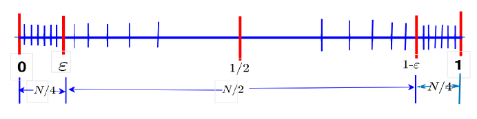
In this section, we have constructed a modified graded mesh for the interval $[0,1]$ to address the reaction-diffusion parabolic problem, incorporating the effects of the perturbation parameter associated with boundary layers on both sides of the domain-specifically, at $r=0$ (left) and $r=1$ (right). The modified graded mesh is generated using a piecewise-defined function within the given interval $[0,1]$. The subintervals $[0,\epsilon ]$ and $[1-\epsilon ,\epsilon ]$ represent the finer regions in the spatial direction, forming a uniform grid divided into $𝒩/4$ segments. In contrast, the interval $[\epsilon ,1-\epsilon ]$ constitutes the coarser region of the graded mesh, characterized by a non-uniform grid obtained through the non-linear equation (12) and subdivided into $𝒩/2$ segments. The nonlinear equation (12) itself is derived using the bisection method.

Figure 1. Modified graded mesh in the spatial direction for $𝒩=32$ and $\epsilon ={10}^{-1}$.

(11) $\{\begin{array}{cc}{\eta }_0=0,\hfill & \\ {\eta }_i=4\epsilon i/𝒩,i=1,2,\mathrm{\dots },𝒩/4\hfill & \\ {\eta }_{i+1}=(1+\sigma h){\eta }_i,i=𝒩/4,\mathrm{\dots },(𝒩/2)-2\hfill & \\ {\eta }_{𝒩/2}=1/2,\hfill & \\ {\eta }_i=1-{\eta }_{𝒩-i},i=(𝒩/2)+1,\mathrm{\dots },𝒩.\hfill & \end{array}$

These equations establish a piecewise function for ${\eta }_i$, where ${\eta }_0$ is explicitly defined as $0,$ ${\eta }_{𝒩/2}$ is explicitly set to $1/2$, and the rest of the values are determined based on the specified conditions. This sequence of values for ${\eta }_i$ varies according to the ranges of $i$, utilizing a non-linear equation involving the parameter $h$ and satisfies the following non-linear equation such that

(12) $$\ln (1/\epsilon )=(𝒩/2)\ln (1+\sigma h).$$

This technique guarantees a precise arrangement of grid points across distinct subintervals within the range $[0,1].$ Within each subinterval $[0,\epsilon ]$ and $[1-\epsilon ,1],𝒩/4$ points are evenly distributed with a step length of $4\epsilon /N$. Here, $𝒩$ denotes the total grid point count, and $\epsilon$ represents a small positive value indicating the width of boundary regions. The selection of $h$ within the central subinterval $[\epsilon ,1-\epsilon ]$ is established iteratively through a non-linear equation $(\text{<a href="\#S3.E12" title="Equation 12 ‣ 3. The modified graded mesh and mesh discretization ‣ A numerical approach for singularly perturbed parabolic reaction-diffusion problem on a modified graded mesh" class="ltx\_ref ltx\_font\_italic"><span class="ltx\_text ltx\_ref\_tag">12</span></a>})$. The mesh length is denoted by $h_i={\eta }_i-{\eta }_{i-1}$ for $i=1,2,\mathrm{\dots },𝒩$.

Remark 5.

The proposed modified graded mesh adheres to the following bounds for mesh size.

$$h_i=\{\begin{array}{cc}4\epsilon /𝒩\text{for}i=1,\mathrm{\cdots },𝒩/4\hfill & \\ \rho h{\eta }_{i-1}\text{for}i=𝒩/4+1,𝒩/2+2,\mathrm{\cdots },3𝒩/4\hfill & \\ 4\epsilon /𝒩\text{for}i=3𝒩/4,3𝒩/4+1,\mathrm{\cdots },𝒩.\hfill & \end{array}$$

Lemma 6.

The mesh described in equation $(\text{<a href="\#S3.E11" title="Equation 11 ‣ 3. The modified graded mesh and mesh discretization ‣ A numerical approach for singularly perturbed parabolic reaction-diffusion problem on a modified graded mesh" class="ltx\_ref"><span class="ltx\_text ltx\_ref\_tag">11</span></a>})$ fulfills the subsequent estimates.

$$|h_{i+1}-h_i|\le \{\begin{array}{cc}𝒞h^2\text{for}i=𝒩/2+1,𝒩/2+2,\mathrm{\cdots },3𝒩/4,\hfill & \\ 0\text{otherwise}.\hfill & \end{array}$$

Proof.

Initially, we investigate the results for $i=0,1,2,\mathrm{\cdots },𝒩/2$. No further establishment is required since the mesh is uniform in this segment.

Now, we have described the following for $i=𝒩/2+1,𝒩/2+2,\mathrm{\cdots },𝒩$ such that

$|h_{i+1}-h_i|$ $=|\rho h{\eta }_i-\rho h{\eta }_{i-1}|,$

$=\rho h|{\eta }_i-{\eta }_{i-1}|,$

$={\rho }^2{h}^2{\eta }_{i-1},$

$\le 𝒞h^2.$

Here, we have taken . ∎

Lemma 7.

The parameter $h$ for the modified graded mesh defined in Equation $(\text{<a href="\#S3.E11" title="Equation 11 ‣ 3. The modified graded mesh and mesh discretization ‣ A numerical approach for singularly perturbed parabolic reaction-diffusion problem on a modified graded mesh" class="ltx\_ref"><span class="ltx\_text ltx\_ref\_tag">11</span></a>})$ adheres to the following bound:

$$h\le 𝒞{𝒩}^{-1}\ln (1/\epsilon ).$$

Proof.

In the mesh partition defined in Equation $(\text{<a href="\#S3.E11" title="Equation 11 ‣ 3. The modified graded mesh and mesh discretization ‣ A numerical approach for singularly perturbed parabolic reaction-diffusion problem on a modified graded mesh" class="ltx\_ref ltx\_font\_italic"><span class="ltx\_text ltx\_ref\_tag">11</span></a>})$, let $Q_1$ and $Q_3$ denote the number of points where the mesh spacing remains constant. It is clear that $Q_1$ and$Q_3$ are bounded above by $C/h$. Conversely, $Q_2$ represents the count of points within the same partition where the mesh steps vary, indicating a non-uniform mesh size. Additionally, we consider ${\eta }_{𝒩/2+1}$, identified as the minimum point for which ${\eta }_i>\epsilon$. Now, we aim to derive an upper limit for $Q_2$. Under the assumption that $\rho h\le 1$, we have

$Q_2$ $={\displaystyle \sum _{𝒩/2+1}^{𝒩}}1={\displaystyle \sum _{𝒩/2+1}^{𝒩}}{({\eta }_{i+1}-{\eta }_i)}^{-1}{\displaystyle {\int }_{{\eta }_i}^{{\eta }_{i+1}}}𝑑\eta ,$

$={\displaystyle \sum _{𝒩/2+1}^{𝒩}}{(h_{i+1})}^{-1}{\displaystyle {\int }_{{\eta }_i}^{{\eta }_{i+1}}}𝑑\eta ,$

$={\displaystyle \sum _{𝒩/2+1}^{𝒩}}{(h\rho {\eta }_i)}^{-1}{\displaystyle {\int }_{{\eta }_i}^{{\eta }_{i+1}}}𝑑\eta ,$

$\le {\displaystyle \sum _{𝒩/2+1}^{𝒩}}{(2/\rho h{\eta }_{i+1})}^{-1}{\displaystyle {\int }_{{\eta }_j}^{{\eta }_{i+1}}}𝑑\eta ,$

because . For any $\eta \in [{\eta }_i,{\eta }_{i+1}]$, we have

$Q_2$ $\le {\displaystyle \sum _{𝒩/2+1}^{𝒩}}2{(\rho h)}^{-1}{\displaystyle {\int }_{{\eta }_i}^{{\eta }_{i+1}}}{\displaystyle \frac{1}{\eta }}𝑑\eta ,$

$\le 2{(\rho h)}^{-1}{\displaystyle {\int }_{\epsilon }^1}{\displaystyle \frac{1}{\eta }}𝑑\eta ,$

$\le 2{(\rho h)}^{-1}\ln (1/\epsilon ).$

Recalling $𝒩=Q_1+Q_2$, we have

$𝒩$ $\le 𝒞/\rho h+2{(\rho h)}^{-1}\ln (1/\epsilon ),$

$𝒩$ $\le 1/h(\rho 𝒞+2\rho \ln (1/\epsilon )),$

$𝒩$ $\le 1/h(𝒞\ln (1/\epsilon )),$

Finally, we get

$$h\le 𝒞{𝒩}^{-1}\ln (1/\epsilon ),$$

where $𝒩$ represents grid points in the $r$-direction. ∎

Remark 8.

From Lemma 6 and Lemma 7 it is clear that the modified graded mesh satisfies

$$|h_{i+1}-h_i|\le C{N}^{-2}{\ln }^2(1/\epsilon )$$

.

3.1. Temporal Discretization

We present mesh with uniform step length in the time direction since layer phenomenon has no effect on the temporal variable $\theta$. The following notation and definition apply to the uniform mesh in the time direction:

$${\mathrm{{\rm Y}}}^{ℳ}=\{{\theta }_s=s\mathrm{\Delta }\theta ,s=0,1,\mathrm{\cdots },M,\mathrm{\Delta }\theta ℳ=𝒯\}.$$

Here $ℳ$ represents the grid points in the temporal direction.

4. Discretization method

Now, we proceed to discretize our domain systematically. We construct a non-uniform grid ${\mathrm{{\rm Y}}}_r^{𝒩}$ on ${\mathrm{{\rm Y}}}_r$, consisting of $𝒩$ mesh points. This grid is formed by placing $𝒩/2$ uniform mesh points within the layer part and $𝒩/2$ mesh points outside the layer part. Additionally, we consider an equidistant grid ${\mathrm{{\rm Y}}}^{ℳ}$ on $[0,𝒯]$ with a uniform step length of $\mathrm{\Delta }\theta$. The discretized domain is then defined as:

$${\mathrm{\Pi }}^{𝒩}={\mathrm{{\rm Y}}}_r^{𝒩}\times {\mathrm{{\rm Y}}}^{ℳ},$$

We now discretize our problem using the aforementioned discretized mesh. We utilize an upwind difference method for spatial derivatives and employ backward Euler for temporal derivatives.

(13) $$\{\begin{array}{cc}(D_{\theta }-\epsilon \frac{D_r^{+}-D_r^{-}}{\widehat{h_i}}+b(i))U_{i,j+1}=f_{i,j+1},i=1,2,\mathrm{\cdots },𝒩-1,\hfill & \\ U_{0,j+1}={\psi }_l({\theta }_{j+1}),\hfill & \\ U_{𝒩,j+1}={\psi }_r({\theta }_{j+1}),\hfill & \\ U_{i,j}={\psi }_b(r_i,{\theta }_j)i=1,2,\mathrm{\cdots },𝒩-1,\hfill & \end{array}$$

by arranging $(\text{<a href="\#S4.E13" title="Equation 13 ‣ 4. Discretization method ‣ A numerical approach for singularly perturbed parabolic reaction-diffusion problem on a modified graded mesh" class="ltx\_ref ltx\_font\_italic"><span class="ltx\_text ltx\_ref\_tag">13</span></a>})$, we will get a tri-diagonal system

(14) $$({\alpha }_{i,j+1})U_{i-1,j+1}+({\beta }_{i,j+1})U_{i,j+1}+({\gamma }_{i,j+1})U_{i+1,j+1}=h_{i,j},$$

where

$$\{\begin{array}{cc}{\alpha }_{i,j+1}=\frac{-\epsilon \mathrm{\Delta }\theta }{h_i{\widehat{h}}_i},\hfill & \\ {\beta }_{i,j+1}=1+\frac{\epsilon \mathrm{\Delta }t}{h_{i+1}{\widehat{h}}_i}+\frac{\epsilon \mathrm{\Delta }t}{h_i{\widehat{h}}_i}+b_i\mathrm{\Delta }\theta ,\hfill & \\ {\gamma }_{i,j+1}=\frac{-\epsilon \mathrm{\Delta }\theta }{h_{i+1}{\widehat{h}}_i},\hfill & \\ h_{i,j}=f_{i,j+1}\mathrm{\Delta }\theta +U_{i,j},\hfill & \\ {\widehat{h}}_i=\frac{h_{i+1}+h_i}{2},\hfill & \end{array}$$

we defined the following parameter of finite difference scheme forward, backward,and central and the mesh function $\tilde{v}(r_i,{\theta }_j)={\tilde{v}}_{i,j}$ such that

$$D_r^{+}{\tilde{v}}_{i,j}=\frac{{\tilde{v}}_{i+1,j}-{\tilde{v}}_{i,j}}{h_{i+1}},D_r^{-}{\tilde{v}}_{i,j}=\frac{{\tilde{v}}_{i,j}-{\tilde{v}}_{i-1,j}}{h_i},$$

$${\delta }_r^2{\tilde{v}}_{i,j}=\frac{(D_r^{+}-D_r^{-}){\tilde{v}}_{i,j}}{{\widehat{h}}_i},D_{\theta }^{-}{\tilde{v}}_{i,j}=\frac{{\tilde{v}}_{i,j}-{\tilde{v}}_{i,j-1}}{h_{i+1}}.$$

4.1. Numerical algorithm

The following algorithm provides the grid construction and the corresponding numerical solution:

Step 1. Given the number of mesh points in the temporal and the spatial direction, $ℳ$ and $𝒩$, respectively, take uniform mesh points in the temporal direction, ${\mathrm{{\rm Y}}}_{j=0}^{ℳ}$ .

Step 2. For the finer part in the spatial direction $(\text{i.e.},[0,\epsilon ],[1-\epsilon ,1]),$ we have the uniform mesh ${\{{\eta }_i\}}_{i=0}^{𝒩/4}$.

Step 3. For the coarser part $(\text{i.e.},[\epsilon ,1-\epsilon ]),$ the graded mesh parameter $h$ is obtained by solving the nonlinear equation (12) by the bisection method.

Step 4. Using the graded mesh parameter $h$, obtain the graded mesh in the interval $[\epsilon ,1-\epsilon ]$ from (11).

Step 5. Set $j=1$.

Step 6. For the value of $j$, solve the tridiagonal system (14) to obtain the solution for the time level $t=j$.

Step 7. $j=j+1$ goto Step 6.

Step 8. If $j=ℳ,$ then stop and mark $U_{i,j},$ as the required solution.

5. Error convergence

Lemma 9.

(Discrete maximum principle) Suppose that $\psi (r_i,{\theta }_j)$ is the mesh function which satisfies $\psi (r_i,{\theta }_j)\ge 0$ on ${\mathrm{\Lambda }}^{𝒩}$. If ${𝔏}_{\epsilon }^{𝒩}\psi (r_i,{\theta }_j)\ge 0$ on $(r_i,{\theta }_j)\in {\mathrm{\Pi }}^{𝒩}$, then $\psi (r_i,{\theta }_j)\ge 0$ on ${\overline{\mathrm{\Pi }}}^{𝒩}$.

Proof.

Let us assume that for all $(r_i,{\theta }_j)\in {\mathrm{\Lambda }}^{𝒩}$, we have $\psi (r_i,{\theta }_j)\ge 0$,and for all $(r_i,{\theta }_j)\in {\mathrm{\Pi }}^{𝒩},{𝔏}_{\epsilon }^{𝒩}\psi (r_i,{\theta }_j)\ge 0$. To contradict we assume that there exists a point $(r_0,{\theta }_0)\in {\mathrm{\Pi }}^N$ such that , and $\psi (r_0,{\theta }_0)$ is a minimum of $\psi$ in ${\mathrm{\Pi }}^N$.

Since, we have assumed that $\psi (r_0,{\theta }_0)$ minimum and also $\psi$ is differentiable, then by applying a second order differential operator ${𝔏}_{\epsilon }^{𝒩}$ on $\psi$ shows that it has upward concavity, which contradicts our supposition that . Also, if $\psi$ attain its minimum on ${\overline{\mathrm{\Pi }}}^N$, then by assumption that $\psi (r_i,{\theta }_j)\ge 0$ for all $(r_i,{\theta }_j)\in {\mathrm{\Lambda }}^{𝒩}$ and hence on ${\overline{\mathrm{\Pi }}}^N,\psi$ must also be non-negative. ∎

Lemma 10.

For any solution $U(r_i,{\theta }_j)$ of $(\text{<a href="\#S4.E13" title="Equation 13 ‣ 4. Discretization method ‣ A numerical approach for singularly perturbed parabolic reaction-diffusion problem on a modified graded mesh" class="ltx\_ref"><span class="ltx\_text ltx\_ref\_tag">13</span></a>})$, we have

(15) $$\Vert U(r_i,{\theta }_j)\Vert \le \left(1+\alpha 𝒯\right)\max (\Vert {𝔏}_{\epsilon }^{𝒩}\Vert ,{\Vert \psi \Vert }_{{\mathrm{\Pi }}^{𝒩}})$$

Proof.

By constructing the barrier function

(16) $${\widehat{U}}^{\pm }(r_i,{\theta }_j)=\left(1+\alpha 𝒯\right)\max (\Vert {𝔏}_{\epsilon }^{𝒩}\Vert ,{\Vert \psi \Vert }_{{\mathrm{\Pi }}^{𝒩}})\pm U(r_i,{\theta }_j).$$

Now, we can obtained the result $(\text{<a href="\#S5.E15" title="Equation 15 ‣ Lemma 10. ‣ 5. Error convergence ‣ A numerical approach for singularly perturbed parabolic reaction-diffusion problem on a modified graded mesh" class="ltx\_ref ltx\_font\_italic"><span class="ltx\_text ltx\_ref\_tag">15</span></a>})$ with apply the Lemma 9 on the result which is defined in $(\text{<a href="\#S5.E16" title="Equation 16 ‣ 5. Error convergence ‣ A numerical approach for singularly perturbed parabolic reaction-diffusion problem on a modified graded mesh" class="ltx\_ref ltx\_font\_italic"><span class="ltx\_text ltx\_ref\_tag">16</span></a>})$. ∎

Theorem 11.

Assume that $u$ and $U$ be the solution of continuous problem $(\text{<a href="\#S1.E1" title="Equation 1 ‣ 1. Introduction ‣ A numerical approach for singularly perturbed parabolic reaction-diffusion problem on a modified graded mesh" class="ltx\_ref"><span class="ltx\_text ltx\_ref\_tag">1</span></a>})$ and discretized problem $(\text{<a href="\#S4.E13" title="Equation 13 ‣ 4. Discretization method ‣ A numerical approach for singularly perturbed parabolic reaction-diffusion problem on a modified graded mesh" class="ltx\_ref"><span class="ltx\_text ltx\_ref\_tag">13</span></a>})$, respectively. Furthermore, both the solutions meet the corners compatibility requirements. Then, the error estimate is given by

(17) $$\max \left|(u-U)(r_i,{\theta }_j)\right|\le 𝒞\left[\mathrm{\Delta }\theta +{𝒩}^{-2}{\ln }^2(1/\epsilon )\right],(r_i,{\theta }_j)\in {\mathrm{\Pi }}^{𝒩}.$$

Here, constant $𝒞$ is free from $𝒩$, $\mathrm{\Delta }\theta$ and $\epsilon$.

Proof.

We consider the following SPPDEs,

(18) $\left(\frac{\partial }{\partial \theta }-\epsilon \frac{{\partial }^2}{\partial r^2}+b(r)\right)u(r,\theta )=f(r,\theta ),$

$u(r,\theta )=u(r,{\theta }_l),r\in {\mathrm{\Lambda }}_b$

$u(0,\theta )={\psi }_0(\theta ),u(1,\theta )={\psi }_1(\theta ),\theta \in [0,𝒯]$

To obtain the numerical solution, we discretize equation (18) employing the upwind finite difference method for spatial derivatives and the backward-Euler scheme for the time derivative.

(19)

where $U_1(r_i,{\theta }_j)$ is the approximate solution obtained over the interval ${\mathrm{\Pi }}^{𝒩}$.

Presently, we partition the solution $u$ of equation (1) into its regular and singular constituents, denoted as $u=\widehat{y}+\widehat{z}$. Additionally, we decompose $\widehat{y}$ as $\widehat{y}=y_0+\epsilon y_1$, where $y_0$ represents the solution to the reduced problem.

$\left(\frac{\partial }{\partial \theta }+b(r,\theta )\right)y_0(r,\theta )=f(r,\theta ),(r,\theta )\in {\mathrm{\Pi }}^{𝒩}.$

$y_0(r,\theta )=u(r,\theta ),$

$y_0(0,\theta )=u(0,\theta ),$

and

${𝔏}_r^{𝒩}{y}_1(r,\theta )=\frac{{\partial }^2{y}_0(r,\theta )}{\partial r^2}$

$y_1(r,\theta )=0,(r,\theta )\in {\mathrm{\Lambda }}_b^{𝒩}$

$y_1(0,\theta )=y_1(1,\theta )=0,(r,\theta )\in {\mathrm{\Lambda }}^N.$

Further $\widehat{y}$ satisfies

${𝔏}_r^{𝒩}\widehat{y}(r,\theta )=f(r,\theta ),(r,\theta )\in {\mathrm{\Pi }}^{𝒩}$

$\widehat{y}(r,\theta )=u(r,\theta ),(r,\theta )\in {\mathrm{\Lambda }}_b^{𝒩}$

$\widehat{y}(0,\theta )=y_0(0,\theta ),\widehat{y}(1,\theta )=y_0(1,\theta ).$

and the singular components $z$ satisfies

${𝔏}_r^{𝒩}\widehat{z}(r,\theta )=0,(r,\theta )\in {\mathrm{\Pi }}^{𝒩}$

$\widehat{z}(r,\theta )=0,(r,\theta )\in {\mathrm{\Lambda }}_b^{𝒩}$

$\widehat{z}(1,\theta )=0,\widehat{z}(0,\theta )={\psi }_l(\theta )-y_0(0,\theta ),\text{on}{\mathrm{\Lambda }}^N.$

We now decompose the numerical solution $U$ of equation (19) into $U=Y+Z$, where $Z$ denotes the singular component of the decomposition, and $Y$ represents the regular component, which is the solution to the subsequent non-homogeneous problem

${𝔏}_r^{𝒩}Y=f(r_i,{\theta }_j),(r_i,{\theta }_j)\in {\mathrm{\Pi }}^{𝒩}$

$Y(r_i,{\theta }_j)=U_1(r_i,{\theta }_j),(r_i,{\theta }_j)\in {\mathrm{\Lambda }}_b^{𝒩}$

$Y(0,{\theta }_j)=\widehat{y}(0,{\theta }_j),Y(1,{\theta }_j)=\widehat{y}(1,{\theta }_j),$

and the singular component $Z$ must satisfy,

${𝔏}_r^{𝒩}Z=0,(r_i,{\theta }_j)\in {\mathrm{\Pi }}^{𝒩}$

$Z(r_i,{\theta }_j)=0,(r_i,{\theta }_j)\in {\mathrm{\Pi }}^{𝒩}$

$Z(1,{\theta }_j)=0,Z(0,{\theta }_j)={\psi }_l({\theta }_j)-\widehat{y}(0,{\theta }_j)\text{on}{\mathrm{\Lambda }}^N.$

Thus, the error can be expressed as:

$$U-u=(Y-\widehat{y})+(Z-\widehat{z})$$

We will now derive the bounds for the smooth and the layer components. To establish the bound for the smooth component, we employ a classical argument. The smooth error component can be written as:

${𝔏}_r^{𝒩}(Y-\widehat{y})$ $=f(r_i,{\theta }_j)-{𝔏}_r^{𝒩}\widehat{y}$

$=-U(r_i,{\theta }_j)+{𝔏}_r^{𝒩}\widehat{y}$

thus we obtain

$${𝔏}_r^{𝒩}(Y-\widehat{y})=-\epsilon (\frac{{\partial }^2}{\partial r^2}-{\delta }_r^2)\widehat{y}+(\frac{\partial }{\partial \theta }-{\delta }_{\theta })\widehat{y}.$$

When taking the absolute values on both sides and applying (17), the preceding inequality becomes,

$$\left|{𝔏}_r^{𝒩}(Y-\widehat{y})\right|\le 𝒞\left(\mathrm{\Delta }\theta +{𝒩}^{-2}{\ln }^2(1/\epsilon )\right)+\epsilon \left|\left(\frac{{\partial }^2}{\partial r^2}-{\delta }_r^2\right)\widehat{y}\right|+\left|\left(\frac{\partial }{\partial \theta }-{\delta }_{\theta }\right)\widehat{y}\right|,$$

also we used the Taylor series expansion such that

$$\le 𝒞\left(\mathrm{\Delta }\theta +{𝒩}^{-2}{\ln }^2(1/\epsilon )\right)+\frac{\epsilon }{12}{\left(r_{i+1}-r_{i-1}\right)}^2\Vert \frac{{\partial }^4\widehat{y}}{\partial r^4}\Vert +\frac{\left({\theta }_j-{\theta }_{j-1}\right)}{2}\Vert \frac{{\partial }^2\widehat{y}}{\partial {\theta }^2}\Vert .$$

On using Remark 8, estimates of derivatives, bounds of mesh length and discrete maximum principle, we have

(20) $$\left|\left(Y-\widehat{y}\right)(r_i,{\theta }_j)\right|\le 𝒞\left[\mathrm{\Delta }\theta +{𝒩}^{-2}{\ln }^2(1/\epsilon )\right].$$

Similar to the continuous variable $z$, the discrete counterpart $Z$ is utilized to estimate the singular component, we have

${𝔏}_r^{𝒩}Z=0,{\theta }_j)\in \mathrm{\Pi }{}^{𝒩}$

$Z(r_i,{\theta }_j)=0,$

$Z(1,{\theta }_j)=0,Z(0,{\theta }_j)={\psi }_l({\theta }_j)-\widehat{y}(0,{\theta }_j).$

The singular component error can be expressed as,

${𝔏}_r^{𝒩}(Z-\widehat{z})$ $={𝔏}_r^{𝒩}Z-{𝔏}_r^{𝒩}\widehat{z},$

$=-\epsilon (\frac{{\partial }^2}{\partial r^2}-{\delta }_r^2)\widehat{z}+(\frac{\partial }{\partial \theta }-{\delta }_{\theta })\widehat{z}$

then the classical estimates gives

$$\left|{𝔏}_r^{𝒩}(Z-\widehat{z})(r_i,{\theta }_j)\right|\le 𝒞\left[\mathrm{\Delta }\theta +{𝒩}^{-2}{\ln }^2(1/\epsilon )\right]$$

The discrete maximum principle is satisfied by the operator ${𝔏}_r^{𝒩}$ and also, due to the uniform boundedness of the inverse operator, the above inequality reduces to,

(21) $$\left|(Z-\widehat{z})(r_i,{\theta }_j)\right|\le 𝒞\left[\mathrm{\Delta }\theta +{𝒩}^{-2}{\ln }^2(1/\epsilon )\right]$$

Combining (20) and (21) completes the proof on prescribed domain. ∎

6. Numerical Experiments

This section contains two examples featuring boundary layers to demonstrate the discussed numerical method. Through tables and graphs, we present the efficiency of the numerical approach. All numerical computations are conducted with $\rho =0.9$. The numerical outcomes validate our theoretical conclusions.

Example 12.

Consider the following parabolic IBVP:

(22) $\{\begin{array}{cc}(\partial u/\partial \theta )-\epsilon {\partial }^{2}u/\partial r^2-2u(r,\theta )=f(r,\theta ),\hfill & \\ (r,\theta )\in (0,1)\times (0,1],\hfill & \\ u(r,0)=u_0(r),\le r\le 1\hfill & \\ u(0,\theta )=\exp (-\theta ),u(1,\theta )=\exp (-(\theta +1/\sqrt{\epsilon }),0\le \theta \le 1.\hfill & \end{array}$

We select the initial data $u_0(r,\theta )$ and the source function $f(r,\theta )$ to match the exact solution $u(r,\theta )=\exp \left(-(\theta +r/\sqrt{\epsilon })\right)$. Moreover, we define the maximum point-wise error $e_{\epsilon }^{𝒩,\mathrm{\Delta }\theta }$ corresponding order of convergence $p_{\epsilon }^{N,\mathrm{\Delta }\theta }$ for each $\epsilon$ as:

$e_{\epsilon }^{𝒩,\mathrm{\Delta }\theta }=$ $\max \left|\left(u-U\right)(r_i,{\theta }_j)\right|,(r_i,{\theta }_j)\in {\mathrm{\Pi }}^{𝒩},$

$p_{\epsilon }^{N,\mathrm{\Delta }\theta }=$ ${\displaystyle \frac{\log (e^{N,\mathrm{\Delta }\theta }/e^{2N,\mathrm{\Delta }\theta /2})}{\log 2}}.$

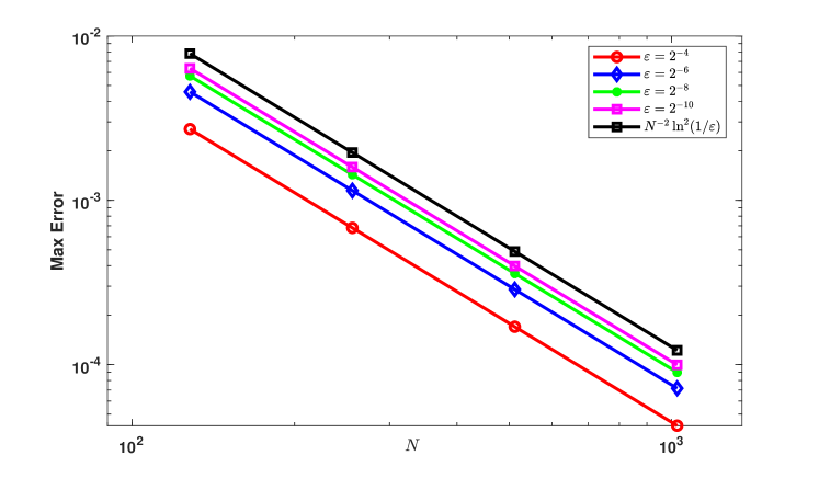
where $u$ and $U$ are exact and approximate solution respectively. We compute the maximum point-wise error $e_{\epsilon }^{𝒩,\mathrm{\Delta }\theta }$ and the order of convergence $p_{\epsilon }^{N,\mathrm{\Delta }\theta }$ for Example 12 using a modified graded mesh and Shishkin mesh, which includes boundary layers at $r=0$ and $r=1$ on both the left and right sides of the domain. We apply the upwind finite difference scheme and summarize the results in Table 1 and Table 2. Our observation from the results in Table 1 and Table 2 is that the scheme exhibits second-order convergence. Additionally, in the log-log plot shown in Fig. 2, it is evident that the maximum point-wise error of the proposed numerical method exhibits a second-order convergence with the perturbation parameter $\epsilon$ in space.

Number of Intervals $N/\mathrm{\Delta }\theta$
$\epsilon$	128/$\frac{1}{10}$	256/$\frac{1}{20}$	512/$\frac{1}{40}$	1024/$\frac{1}{80}$
$2^{-4}$	$1.5547E-03$	$3.9188E-04$	$9.8239E-05$	$2.4586E-05$
	$1.9882$	$1.9960$	$1.9985$
$2^{-6}$	$1.4792E-03$	$3.7299E-04$	$9.3163E-05$	$2.3317E-05$
	$1.9876$	$2.0013$	$1.9983$
$2^{-8}$	$1.4000E-03$	$3.5012E-04$	$8.7423E-05$	$2.1836E-05$
	$1.9995$	$2.0018$	$2.0013$
$2^{-10}$	$1.2888E-03$	$3.2081E-04$	$7.9953E-05$	$1.9953E-05$
	$2.0062$	$2.0045$	$2.0025$
$e_{\epsilon }^{𝒩,\mathrm{\Delta }\theta }$	$1.2888E-03$	$3.2081E-04$	$7.9953E-05$	$1.9953E-05$
$p_{\epsilon }^{N,\mathrm{\Delta }\theta }$	$2.0062$	$2.0045$	$2.0025$

Table 1. Maximum point-wise errors and order of convergence on a modified graded mesh for Example 12.

In order to compare our results with the well established Shishkin mesh [19], we define the the Shishkin mesh for the problem considered as follows. The Shishkin mesh is a piecewise uniform mesh, depends on two transition points which are defined by means of the transition parameter.

(23) $$\sigma =\min \{1/4,{\sigma }_0\sqrt{\epsilon }\ln 𝒩\},$$

where ${\sigma }_0$ is a constant to be fixed later. A uniform mesh is placed in $[0,\sigma ]$, $[\sigma ,1-\sigma ]$ and $[1-\sigma ,1],$ such that $r_0=0,r_{𝒩/4}=\sigma$, $r_{3𝒩/4}=1-\sigma ,$ and $r_{𝒩}=1.$ Therefore the mesh points are given by $r_i=4i\sigma /𝒩,$ for $i=0,1,\mathrm{\dots },𝒩/4,$ $r_i=\sigma +2(i-𝒩)(1-2\sigma )/𝒩,$ for $i=𝒩/4+1,\mathrm{\dots },3𝒩/4,$ and $r_i=1-\sigma +4(i-3𝒩/4)\sigma /𝒩,$ for $i=3𝒩/4+1,\mathrm{\dots },𝒩.$

Number of Intervals $N/\mathrm{\Delta }\theta$
$\epsilon$	128/$\frac{1}{10}$	256/$\frac{1}{20}$	512/$\frac{1}{40}$	1024/$\frac{1}{80}$
$2^{-4}$	$1.6096E-03$	$4.0509E-04$	$1.0144E-04$	$2.5371E-05$
	$1.9903$	$1.9975$	$1.9993$
$2^{-6}$	$1.6420E-03$	$4.1335E-04$	$1.0352E-04$	$2.5891E-05$
	$1.9900$	$1.9974$	$1.9993$
$2^{-8}$	$1.7637E-03$	$4.4458E-04$	$1.1138E-04$	$2.7862E-05$
	$1.9881$	$1.9969$	$1.9991$
$2^{-10}$	$1.8389E-03$	$4.8298E-04$	$1.2641E-04$	$3.3124E-05$
	$1.9288$	$1.9339$	$1.9321$
$e_{\epsilon }^{𝒩,\mathrm{\Delta }\theta }$	$1.8389E-03$	$4.8298E-04$	$1.2641E-04$	$3.3124E-05$
$p_{\epsilon }^{N,\mathrm{\Delta }\theta }$	$1.9288$	$1.9339$	$1.9321$

Table 2. Maximum point-wise errors and order of convergence on a Shishkin mesh for Example 12.

Example 13.

Consider the following problem

$u_{\theta }-\epsilon u_{rr}+((1+r^2)/2)u={\text{e}}^{\theta }-1+sin(\pi r),(r,\theta )\in (0,1)\times (0,1],$

with homogeneous initial and boundary conditions.

In Example 13, an exact solution is unavailable. Consequently, to assess the maximum point-wise error and determine the order of convergence for the computed solution, we employ the double mesh principle. This involves considering $2N$ intervals in the spatial direction and $2M$ intervals in the temporal direction. We obtain the numerical solution $\tilde{U}(r_i,{\theta }_j)$ on the mesh ${\overline{\mathrm{\Pi }}}^{2N}={\overline{\mathrm{{\rm Y}}}}_r^{2N}\times {\overline{\mathrm{{\rm Y}}}}^{2M}$, where $i=1,2,\mathrm{\cdots },N$. Notably, each $i$th point of the mesh ${\mathrm{{\rm Y}}}_r^N$ coincides with the $2i$th point of the mesh ${\overline{\mathrm{{\rm Y}}}}_r^{2N}$.

The maximum point-wise error for each $\epsilon$ is defined by,

$$e_{\epsilon }^{N,\mathrm{\Delta }\theta }=\max \left|(U-\tilde{U})(r_i,{\theta }_j)\right|,(r_i,{\theta }_j)\in {\mathrm{\Pi }}^N,$$

and the order of convergence is given by

$$p_{\epsilon }^{N,\mathrm{\Delta }\theta }=\frac{\log (e^{N,\mathrm{\Delta }\theta }/e^{2N,\mathrm{\Delta }\theta /2})}{\log 2}.$$

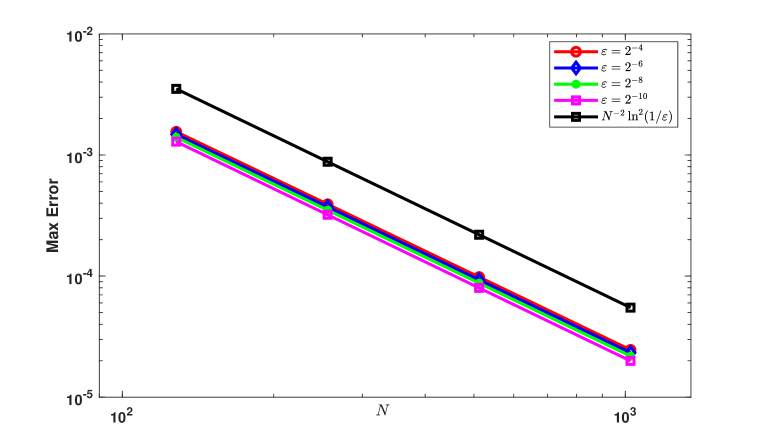
Similarly, we compute the maximum point-wise error $e_{\epsilon }^{𝒩,\mathrm{\Delta }\theta }$ and the order of convergence $p_{\epsilon }^{N,\mathrm{\Delta }\theta }$ for Example 13 using a modified graded mesh and Shishkin mesh, which includes boundary layers at $r=0$ and $r=1$ on both the left and right sides of the domain. We apply the upwind finite difference scheme and summarize the results in Table 3 and Table 4. Our observation from the results in Table 3 and Table 4. is that the scheme exhibits second-order convergence with the perturbation parameter $\epsilon$ in space. Additionally, in the log-log plot shown in Fig. 2, it is evident that the maximum point-wise error of the proposed numerical method exhibits a second-order uniform convergence in the perturbation parameter $\epsilon$ in space.

Number of Intervals $N/\mathrm{\Delta }\theta$
$\epsilon$	128/$\frac{1}{10}$	256/$\frac{1}{20}$	512/$\frac{1}{40}$	1024/$\frac{1}{80}$
$2^{-4}$	$2.7121E-03$	$6.7948E-04$	$1.6990E-04$	$4.2469E-05$
	$1.9969$	$1.9997$	$2.0002$
$2^{-6}$	$4.5714E-03$	$1.1459E-03$	$2.8663E-04$	$7.1668E-05$
	$1.9962$	$1.9992$	$1.9998$
$2^{-8}$	$5.7130E-03$	$1.4323E-03$	$3.5830E-04$	$8.9590E-05$
	$1.9960$	$1.9990$	$1.9998$
$2^{-10}$	$6.3522E-03$	$1.5926E-03$	$3.9840E-04$	$9.9615E-05$
	$1.9959$	$1.9991$	$1.9998$
$e_{\epsilon }^{𝒩,\mathrm{\Delta }\theta }$	$6.3522E-03$	$1.5926E-03$	$3.9840E-04$	$9.9615E-05$
$p_{\epsilon }^{N,\mathrm{\Delta }\theta }$	$1.9959$	$1.9991$	$1.9998$

Table 3. Maximum point-wise errors and order of convergence on a modified graded mesh for Example 13.

Number of Intervals $N/\mathrm{\Delta }\theta$
$\epsilon$	128/$\frac{1}{10}$	256/$\frac{1}{20}$	512/$\frac{1}{40}$	1024/$\frac{1}{80}$
$2^{-4}$	$5.7176E-03$	$1.6558E-03$	$4.2963E-04$	$1.0843E-04$
	1.7878	1.9463	1.9862
$2^{-6}$	$1.6010E-02$	$4.0517E-03$	$1.0159E-03$	$2.5417E-04$
	1.9823	1.9957	1.9989
$2^{-8}$	$2.7172E-02$	$6.8564E-03$	$1.7181E-03$	$4.2978E-04$
	1.9865	1.9966	1.9991
$2^{-10}$	$3.3892E-02$	$8.5641E-03$	$2.1467E-03$	$5.3704E-04$
	1.9845	1.9962	1.9990
$e_{\epsilon }^{𝒩,\mathrm{\Delta }\theta }$	$3.3892E-02$	$8.5641E-03$	$2.1467E-03$	$5.3704E-04$
$p_{\epsilon }^{N,\mathrm{\Delta }\theta }$	$1.9959$	$1.9991$	$1.9998$

Table 4. Maximum point-wise errors and order of convergence on a Shishkin mesh for Example 13.

Results by proposed method on the modified graded mesh
Number of Intervals $N/\mathrm{\Delta }\theta$
$\left(\epsilon =2^{-4},2^{-6},2^{-8},2^{-10}\right)$	128/$\frac{1}{10}$	256/$\frac{1}{20}$	512/$\frac{1}{40}$	1024/$\frac{1}{80}$
$e_{\epsilon }^{𝒩,\mathrm{\Delta }\theta }$	$2.7121E-03$	$6.7948E-04$	$1.6990E-04$	$4.2469E-05$
$p_{\epsilon }^{N,\mathrm{\Delta }\theta }$	$1.9969$	$1.9997$	$2.0002$
Results by proposed method on the Shishkin mesh
Number of Intervals $N/\mathrm{\Delta }\theta$
$\left(\epsilon =2^{-4},2^{-6},2^{-8},2^{-10}\right)$	128/$\frac{1}{10}$	256/$\frac{1}{20}$	512/$\frac{1}{40}$	1024/$\frac{1}{80}$
$e_{\epsilon }^{𝒩,\mathrm{\Delta }\theta }$	$3.3892E-02$	$8.5641E-03$	$2.1467E-03$	$5.3704E-04$
$p_{\epsilon }^{N,\mathrm{\Delta }\theta }$	$1.9959$	$1.9991$	$1.9998$
Results by [19]
Number of Intervals $N/\mathrm{\Delta }\theta$
$\left(\epsilon =2^{-4},2^{-6},2^{-8},2^{-10}\right)$	128/$\frac{1}{10}$	256/$\frac{1}{20}$	512/$\frac{1}{40}$	1024/$\frac{1}{80}$
$e_{\epsilon }^{𝒩,\mathrm{\Delta }\theta }$	$1.6600E-03$	$5.7800E-04$	$1.9200E-04$	$5.9500E-05$
$p_{\epsilon }^{N,\mathrm{\Delta }\theta }$	$1.5270$	$1.5900$	$1.6900$

Table 5. Comparison of Maximum uniform errors and order of uniform convergence for Example 13.

Figure 2. Log-log plot for Example 12 in Fig. 2 and for Example 13 in Fig. 2.

7. Discussion and Conclusions

In this article, for the first time, we propose a modified graded mesh for reaction-diffusion problems that provides second-order uniform convergence with respect to the perturbation parameter. We have presented effective numerical approaches in this work that are based on a modified graded mesh. We have presented upwind finite difference schemes on modified graded mesh and Shishkin mesh. In order to verify the theoretical estimation established, we conduct numerical experiments for two test problems for various values of $\epsilon$, and step sizes $N$ and $M$. In order to find maximum point-wise error and corresponding order of convergence, we double the number of mesh points in the time and spatial direction for the proposed schemes on the modified graded mesh and Shishkin mesh. Through this procedure we get the second-order convergence. These can be observed from the results presented in Table 1 and Table 2 for Example 12 and Table 3, Table 4 for Example 13. From the above tables it can be confirmed that overall second order uniform convergence. Corresponding log-log plot are provided for the Example 12 and Example 13. Fig. 2 shows the overall second order of convergence for various values of $\epsilon$ with the upwind finite difference scheme on modified graded mesh and Shishkin mesh. Table 5 display comparison of the proposed scheme with the previous works. It is observed the proposed scheme is better than those considered in [19]. The uniform convergence of the proposed methods is shown by the numerical results obtained for the test problems. The ability to build higher-order, more time-accurate numerical schemes using the current setting is a feasible extension that may be used to improve accuracy while reducing computing costs. Finally, numerical outcomes supports the theoretical findings.

Funding: The first author Mr. Kishun Kumar Sah conveys his profound gratitude to the Department of Science and Technology, Govt. of India for providing INSPIRE fellowship (IF 190722).

Data Availability: Enquiries about data availability should be directed to the authors.

Acknowledgements.

The authors would like to thank the referees and editor for their useful remarks, which contributed to improving the quality of this article.