A Comparative Study on Balanced Truncation and Projection onto the Dominant Eigenspace of the Gramian Using Laguerre Functions

Abstract.

This paper presents a comparative analysis of two model reduction techniques: balanced truncation and projection onto the dominant eigenspace of the Gramian. Both methods are evaluated through the lens of Laguerre functions which is a reduction technique based on Laguerre function expansion, that approximates the low-rank factors of the Controllability and Observability Gramians to produce approximately balanced systems without solving Lyapunov equations. We demonstrate the effectiveness of each approach in reducing the complexity of linear time-invariant (LTI) systems while preserving system dynamics. Numerical experiments highlight the strengths and weaknesses of both methods, showcasing their applicability to large-scale systems. By thoroughly analyzing both methods in conjunction with Laguerre functions, we contribute to the ongoing discourse in the field and lay the groundwork for future advancements in model reduction techniques.

1. Introduction

We consider a first-order generalized LTI continuous-time dynamical system:

(1)

where $A\in {ℝ}^{n\times n}$, $B\in {ℝ}^{n\times p}$, and $C\in {ℝ}^{m\times n}$ represent the system, input, and output matrices, respectively. We also have $x(t)\in {ℝ}^n$, $u(t)\in {ℝ}^p$, and $y(t)\in {ℝ}^m$, which are the vectors of system states, inputs, and outputs, respectively. Due to the limitations of computational time and computer memory, simulation and analysis for large-scale systems like system (1) are difficult. To avoid these complexities, reducing the system is indispensable. Model order reduction [MOR] [antoulas2005approximation, moore1981principal, freund2003model] is a critical aspect of control systems design, particularly for large-scale linear time-invariant (LTI) systems [antoulas2005approximation, benner2008numerical]. In MOR techniques, we replace system (1) with a significantly low-dimensional system as below:

(2)

where $E_r,A_r\in {ℝ}^{r\times r}$, $B_r\in {ℝ}^{r\times m}$, $C_r\in {ℝ}^{p\times r}$ are the reduced-dimensional matrices corresponding to the above system (1).

Our goal is to make the approximation error $\Vert G-G_r\Vert$ sufficiently small, where $G$ and $G_r$ are the transfer functions [Hindi_1987] of the initial large system and reduced system, respectively. The transfer functions are given by:

(3) $$G(s)=C{(sE-A)}^{-1}B,G_r(s)=C_r{(s{E}_r-A_r)}^{-1}{B}_r.$$

Traditional MOR techniques [datta2004numerical, schilders2008introduction, uddin2019computational] often rely on solving Lyapunov equations [benner2008numerical, benner2011efficient] to compute the solution matrices called Controllability and Observability Gramians [uddin2017structure]. However, for large-scale systems, solving the Lyapunov equations is computationally intensive. Our approach circumvents this by employing Laguerre functions, which allow the direct construction of low-rank factors of the matrix exponential functions [xiao2022model, xiao2023laguerre]. This method reduces computational complexity and maintains high accuracy in the reduced-order models.

Among the various methods available, balanced truncation [BT] [moore1981principal, gugercin2004survey] and projection onto the dominant eigenspace of the Gramian [PDEG] [hasansolution, uddin2015computational] are two widely studied approaches that offer distinct advantages depending on the application context.

BT method is a well-established method that leverages the controllability and observability Gramians to identify and retain the most significant states of the system. By focusing on the dominant modes, balanced truncation ensures that the reduced model maintains the essential dynamics of the original system. This approach is particularly useful when dealing with systems where maintaining stability and transient response is paramount.

On the other hand, PDEG method provides a more direct method for reducing model complexity. By utilizing the eigenvectors corresponding to the largest eigenvalues of the Gramian, this technique effectively captures the primary dynamics of the system in a lower-dimensional space [penzl2006algorithms]. This projection method can be particularly advantageous for systems where computational efficiency is critical [antoulas2001survey, benner2015survey] as it allows for rapid computations with minimal loss of accuracy. Among these two methods, BT provides comparatively better approximation [saiduzzaman2022comparative]. In this paper, we undertake a comparative analysis of these two model reduction techniques, specifically examining their performance when integrated with Laguerre functions. Laguerre functions have garnered attention due to their ability to represent system dynamics compactly and efficiently making them an ideal choice for model reduction tasks.

In this study, we contribute to system order reduction by utilizing BT and PDEG for continuous-time systems, utilizing the Laguerre function expansion—an aspect not previously explored. While the BT method has been applied alongside the Laguerre function in [xiao2023laguerre] for discrete-time systems, our approach is the first to extend this concept to continuous-time systems. Additionally, we conduct a comparative analysis of both methods to identify the most effective approach for system reduction. Specifically, the study presents a detailed evaluation showing that BT, when combined with Laguerre expansion, results in better performance in terms of model reduction compared to PDEG. By providing a thorough comparison of the two methods, the paper demonstrates that the Laguerre expansion can enhance the accuracy and efficiency of the reduction process, especially for large-scale systems. This comparative study and the conclusion that BT outperforms PDEG in certain contexts is a novel aspect of the paper that distinguishes it from existing research.

To validate the effectiveness of our approach, we conduct a series of numerical experiments on two different models. These experiments aim to assess how accurately and efficiently the reduced-order models (ROMs) perform relative to the original model. The residue of this paper is synchronized as follows.
We provide a brief framework of matrix exponential approximation using Laguerre functions in Section 2. The decomposition of gramian matrices $P$ and $Q$ using Laguerre expansion is derived in Section 3. Section 4 and Section 5 provide the BT and PDEG methods applying Laguerre function. Basic algorithms for both methods are presented in Section 6. Section 7 presents the results and discussion showcasing the performance and accuracy of the methods using numerical tables and graphical displays. Finally, Section 8 concludes our discussion by providing a comprehensive overview of our discoveries, offering insights, and proposing avenues for future research.

2. Matrix Exponential Function Approximation using Laguerre functions

Laguerre functions are a set of orthogonal polynomials that are solutions to Laguerre’s differential equation. The generalized (or associated) Laguerre polynomials $L_n^{(\lambda )}(x)$ can be defined using the following generating function:

$$\sum _{n=0}^{\mathrm{\infty }}{L}_n^{(\lambda )}(x)t^n=\frac{e^{-xt/(1-t)}}{{(1-t)}^{\lambda +1}},$$

where $L_n^{(\lambda )}(x)$ is the $n$-th generalized Laguerre polynomial.

The standard Laguerre polynomials can be expressed explicitly using Rodrigues’ formula:

$$L_n(x)=\frac{e^x}{n!}\frac{d^n}{d{x}^n}\left(e^{-x}{x}^n\right).$$

These polynomials are used to define the scaled Laguerre functions as follows:

$${\varphi }_i^{(\lambda )}(t)=\sqrt{2\lambda }{e}^{-\lambda t}{L}_i(2\lambda t).$$

In this definition, $\lambda$ serves as a scaling coefficient that governs the attenuation rate of the exponential term $e^{-\lambda t}$, and $L_i(2\lambda t)$ denotes the Laguerre polynomial computed at $2\lambda t$.

Within the framework of frequency domain analysis, the Laplace transforms of scaled Laguerre functions are formulated as follows:

$${\mathrm{\Phi }}_i^{(\lambda )}(s)=ℒ({\varphi }_i^{(\lambda )}(t))=\frac{\sqrt{2\lambda }}{s+\lambda }{\left(\frac{s-\lambda }{s+\lambda }\right)}^i,\text{for }i=0,1,\mathrm{\dots }$$

For values of $a$ where , the expansion of $e^{\lambda t}$ in terms of Laguerre functions is given by:

$$e^{\lambda t}=\sum _{k=0}^{\mathrm{\infty }}{a}_k{\varphi }_k^{(\lambda )}(t),t\ge 0,$$

where the coefficients ${\{a_k\}}_{k=0}^{\mathrm{\infty }}$ are defined by:

$$a_k={\int }_0^{\mathrm{\infty }}{e}^{\lambda t}{\varphi }_k^{(\lambda )}(t)𝑑t=\frac{\sqrt{2\lambda }}{\lambda -a}{\left(\frac{a+\lambda }{a-\lambda }\right)}^k$$

$$={(-1)}^k\sqrt{2\lambda }{(a+\lambda )}^k{(\lambda -a)}^{-(k+1)}.$$

For , $e^{At}$ is expressed as

$$e^{At}=\sum _{k=0}^{\mathrm{\infty }}{A}_k{\varphi }_k^{(\lambda )}(t),$$

where ${\{A_k\}}_{k=0}^{\mathrm{\infty }}$ are coefficient matrices defined by:

$$A_k={(-1)}^k\sqrt{2\lambda }{(\lambda I+A)}^k{(\lambda I-A)}^{-(k+1)},$$

where $I$ denotes the unit matrix.

Then $A_i$ can be found using the recursive formula as follows, applying different values of $k$ in the expression for $A_k$ described earlier.

$A_0$ $={(-1)}^0\sqrt{2\lambda }{(\lambda I+A)}^0{(\lambda I-A)}^{-1}=\sqrt{2\lambda }{(\lambda I-A)}^{-1}$

$A_1$ $=(-1)\sqrt{2\lambda }(\lambda I+A){(\lambda I-A)}^{-2}=\sqrt{2\lambda }{(\lambda I-A)}^{-1}(\lambda I+A){(A-\lambda I)}^{-1}$

$=(\lambda I+A){(A-\lambda I)}^{-1}{A}_0$

$A_2$ $=\sqrt{2\lambda }{(\lambda I+A)}^2{(\lambda I-A)}^{-3}$

$=\sqrt{2\lambda }{(\lambda I-A)}^{-1}(\lambda I+A){(A-\lambda I)}^{-1}(\lambda I+A){(A-\lambda I)}^{-1}$

$=(\lambda I+A){(A-\lambda I)}^{-1}{A}_1$

Similarly, we can write,

$A_i$ $=(\lambda I+A){(A-\lambda I)}^{-1}{A}_{i-1},i=1,2,\mathrm{\dots }N-1.$

3. Decomposition of Gramian Matrices P and Q Using Laguerre expansion

We introduce an approximation of the Grampians $P$ and $Q$ utilizing Laguerre expansion. Initially, we express $e^{At}B$ using a finite set of Laguerre functions in the following approximate manner:

$$e^{At}B\approx \sum _{i=0}^{N-1}{A}_{i}B{\varphi }_i^{\lambda }(t),$$

Then, $P$ can be expressed as:

$P$ $={\displaystyle {\int }_0^{\mathrm{\infty }}}{e}^{At}B{B}^T{e}^{A^{T}t}𝑑t$

$={\displaystyle {\int }_0^{\mathrm{\infty }}}(e^{At}B){(e^{At}B)}^T𝑑t$

$\approx {\displaystyle {\int }_0^{\mathrm{\infty }}}{\displaystyle \sum _{i=0}^{N-1}}{A}_{i}B{\varphi }_i^{\lambda }(t){\left({\displaystyle \sum _{i=0}^{N-1}}{A}_{i}B{\varphi }_i^{\lambda }(t)\right)}^{T}dt$

Given the orthogonal property of the Laguerre functions, the matrix $P$ can be approximated as $P\approx F{F}^T$, where

(4)

Analogously to the factorization of $P$, the observability Gramian $Q$ can be represented in a low-rank format as follows: $Q\approx G{G}^T$,where

(5)

4. Laguerre-based Balanced truncation method

The objective of BT is to derive a ROM by eliminating states that pose challenges in terms of both control and observation. In that case, the state according to the smaller singular values is hard to control and observe, and truncating the smaller singular values makes the system easily controllable and observable. The solutions corresponding to the system (1), known as the Controllability Gramian ($P$) and the Observability Gramian ($Q$), are calculated from equations (4) and (5) respectively.

Now, we perform the Singular Value Decomposition (SVD) on the product $G^{T}F$:

$$\text{SVD}(G^{T}F)=U\mathrm{\Sigma }{V}^T$$

Here, $U$ and $V$ are the left and right singular vectors, and $\mathrm{\Sigma }$ is the diagonal matrix of singular values. Next, retain the first $r$ columns of $U$ and $V$ and the first $r\times r$ block of $\mathrm{\Sigma }$:

$$U_r=U(:,1:r),V_r=V(:,1:r),{\mathrm{\Sigma }}_r=\mathrm{\Sigma }(1:r,1:r)$$

Then we compute the projection matrices $T_R$ and $T_L$ based on the truncated singular vectors:

$$T_R:=F{V}_r{\mathrm{\Sigma }}_r^{-1/2},T_L:=G{U}_r{\mathrm{\Sigma }}_r^{-1/2}$$

Finally, the projection matrices, construct the reduced-order model (ROM) by computing the reduced system matrices as:

$$E_r=T_L^{T}E{T}_R,A_r=T_L^{T}A{T}_R,B_r=T_L^{T}B,C_r=C{T}_R$$

The complete reduction procedure is provided in Algorithm 1.

5. Projection onto the dominant eigenspace of the Gramian using Laguerre function expansion

In PDEG method we project the system onto the dominant eigenvalues of the system’s Gramians. At first we calculate the Controllability Gramian factor $F_L$ and the Observability Gramian factor $G_L$ using (4) and (5) respectively. Once we have computed the Gramians as $P=F_L{F}_L^T$ or $Q=G_L{G}_L^T$, we perform a Singular Value Decomposition (SVD) to obtain the orthogonal vectors $U$ and $V$, where:

$$P=U\mathrm{\Sigma }{U}^T\text{or}Q=V\mathrm{\Lambda }{V}^T$$

Here, $U$ and $V$ are orthogonal matrices containing the left and right singular vectors, respectively, and $\mathrm{\Sigma }$ and $\mathrm{\Lambda }$ are diagonal matrices containing the singular values.

After performing the SVD, we truncate the vectors corresponding to the smaller singular values, as they are deemed less significant to the system dynamics. This step reduces the rank of the system, focusing on the dominant modes that contribute significantly to the system’s behavior. We retain the first $r$ dominant singular values and the corresponding orthogonal vectors.

Using the truncated orthogonal vectors, we form the low-rank factors that define the reduced-order model.

Let $W$ denote the matrix containing the first $r$ dominant vectors (columns of $U$ or $V$):

$$W:=U(:,1:r)\text{or}W:=V(:,1:r)$$

With $W$ constructed, we can now project the original system onto the reduced subspace to obtain the ROM as:

$$E_r=W^{T}EW,A_r=W^{T}AW,B_r=W^{T}B,C_r=CW$$

Here, $E_r$, $A_r$, $B_r$, and $C_r$ represent the system matrices of the reduced-order model, and the rank $r$ determines the reduced system’s order. Algorithm 2 presents the whole process.

6. Basic Algorithms

Two essential algorithms underpin the Laguerre-based approach, providing distinct yet complementary functionalities. The first algorithm focuses on the BT method, where a square-root process is integral to the simulation. This technique efficiently handles transformations critical to achieving stable and accurate results within the framework of the Laguerre function. By addressing potential numerical instabilities, Algorithm 1 ensures the robust implementation of the square-root process, thereby enhancing overall computational reliability.

0:  Matrices $E$, $A$, $B$, $C$; desired reduced order $r$

0:  Reduced-order model matrices $E_r$, $A_r$, $B_r$, $C_r$

1:  Compute the controllability Gramian $F$ and observability Gramian $G$ using equations (4) and (5)

2:  Perform the singular value decomposition (SVD):

$$\text{SVD}(G^{\top }F)=U\mathrm{\Sigma }{V}^{\top }$$

3:  Extract the leading $r$ singular components:

$$U_r=U(:,1:r),V_r=V(:,1:r),{\mathrm{\Sigma }}_r=\mathrm{\Sigma }(1:r,1:r)$$

4:  Compute the projection matrices:

$$T_R=F{V}_r{\mathrm{\Sigma }}_r^{-1/2},T_L=G{U}_r{\mathrm{\Sigma }}_r^{-1/2}$$

5:  Construct the reduced-order model (ROM):

$$E_r=T_L^{\top }E{T}_R,A_r=T_L^{\top }A{T}_R,B_r=T_L^{\top }B,C_r=C{T}_R$$

Algorithm 1 Laguerre-based Square-root Balanced Truncation (BT) Method

The second algorithm caters to the PDEG method, tailored specifically for the Laguerre function expansion. This approach is designed to optimize the representation of functions or solutions by leveraging the orthogonal properties of Laguerre polynomials. Algorithm 2 systematically incorporates this expansion, making it especially suitable for problems requiring high precision in solving differential equations.

0:  Matrices $E$, $A$, $B$, $C$; desired reduced order $r$

0:  Reduced-order model matrices $E_r$, $A_r$, $B_r$, $C_r$

1:  Compute the controllability Gramian $P$ and observability Gramian $Q$ using equations (4) and (5)

2:  Compute the singular value decomposition (SVD) of either $P$ or $Q$:

$$\text{SVD}(P)=U\mathrm{\Sigma }{U}^{\top }\text{or}\text{SVD}(Q)=V\mathrm{\Sigma }{V}^{\top }$$

3:  Select the dominant $r$ modes:

$$W=U(:,1:r)\text{or}W=V(:,1:r)$$

4:  Construct the reduced-order model (ROM):

$$E_r=W^{\top }EW,A_r=W^{\top }AW,B_r=W^{\top }B,C_r=CW$$

Algorithm 2 Laguerre-based Proper Orthogonal Decomposition with Energy Gramians (PDEG) Method

7. Results and discussion

This section provides a detailed summary of the experimental results. The algorithms were implemented using MATLAB (R2021a), ensuring robust computational efficiency and accuracy.

Two data models were selected for evaluation: the CD player model, also known as the classical CD player (CDP) model, which has been widely used in various literature over the years to test the efficiency of MOR methods for LTI dynamical systems. The task in this model is to construct a controller that ensures the laser stays pointed at the track of pits on a rotating CD. The system consists of a swing arm with a lens mounted on it via two horizontal leaf springs. The rotation of the arm in the horizontal plane enables reading of the spiral-shaped disc tracks, and the suspended lens focuses the laser on the disc. The challenge arises from the disc’s imperfect flatness and irregularities in the spiral track, requiring a low-cost controller that improves the servo-system’s speed and makes it less sensitive to external shocks.

The second model is the ISS model, known as the International Space Station (ISS) model, which is used in model order reduction to represent the dynamic behavior and control of the space station, capturing its complex interactions with external forces such as gravity and atmospheric drag. This model is often simplified in model order reduction techniques to improve computational efficiency while retaining the essential dynamics for control and simulation purposes.

Both the CDplayer and ISS models are formulated as linear time-invariant (LTI) systems in standard state-space form as (1). For the CDplayer model, which originates from a second-order mass-spring-damper mechanical system, the equations are initially:

$$M\ddot{q}(t)+D\dot{q}(t)+Kq(t)=Bu(t),y(t)=Cq(t),$$

and are converted into first-order form for reduction.

The ISS model is directly modeled in first-order LTI form, representing the space station’s dynamic behavior under external forces.

For both models, the same algorithmic inputs were used: damping parameter $\alpha =0.1002$, 10 iterations, a reduced order of 6 for the CDplayer model, and 15 for the ISS model. Model reduction was performed using Balanced Truncation, which retains the most energetically significant states based on Hankel singular values. Specifically, the top 6 dominant singular values were retained for the CDplayer model, and the top 15 for the ISS model, corresponding to the chosen reduced dimensions. These values represent the most significant dynamic modes of each system.

For the reduction process applied to the CDplayer model, the parameter $\alpha =0.1002$ was used, with 10 iterations and a target reduced dimension of 6. The same parameter and number of iterations were applied to the ISS model, but the reduced dimension was set to 15. These settings were chosen to ensure consistency in the experimental framework while addressing the specific characteristics of each data model.

The errors derived from the BT and PDEG methods for both models are summarized in Table 1 and Table 2. The results clearly demonstrate that the BT method consistently delivers superior accuracy compared to the PDEG method across both models. This trend is evident from the numerical error values, which highlight the BT method’s effectiveness in achieving precise dimensional reductions while minimizing inaccuracies.

Error	BT	PDEG
Absolute Error	$3.4649\times {10}^{-4}$	$2.204\times {10}^{-1}$
Relative Error	$7.3858\times {10}^{-9}$	$4.6978\times {10}^{-6}$

Table 1. Error comparison between BT and PDEG method for CDplayer Model.

Error	BT	PDEG
Absolute Error	$6.0\times {10}^{-3}$	$1.7\times {10}^{-2}$
Relative Error	$1.926\times {10}^{-1}$	$5.484\times {10}^{-1}$

Table 2. Error comparison between BT and PDEG method for ISS Model.

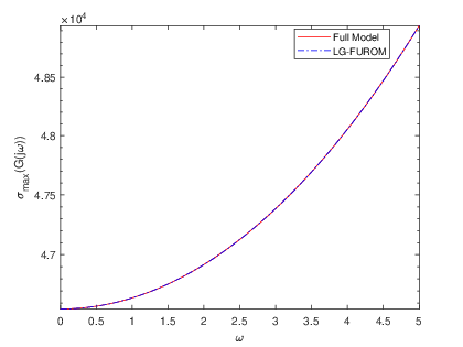
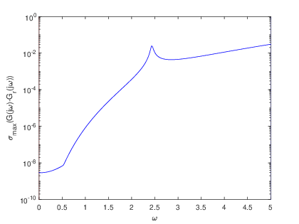
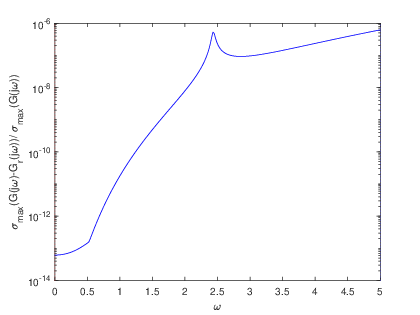
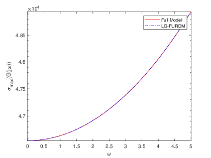
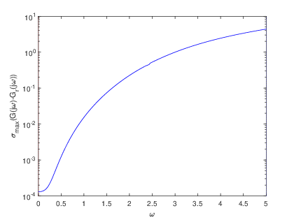
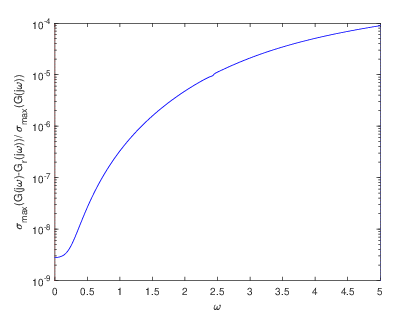
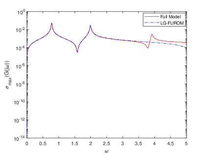
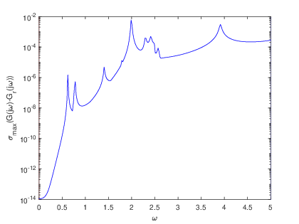
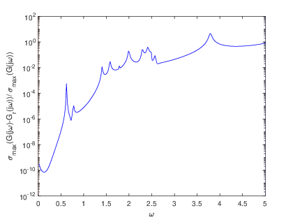
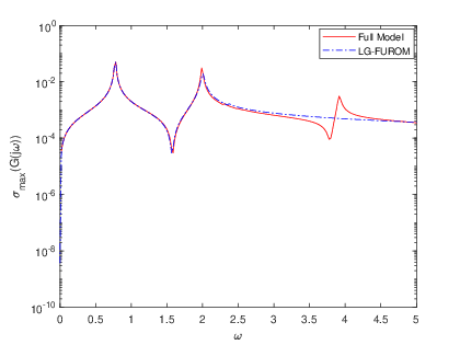
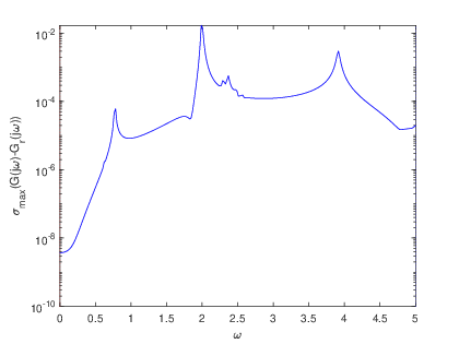
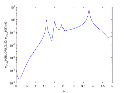
To complement the tabular results, graphical representations were generated to illustrate the reduction process and the associated error estimations. Fig. 2 and Fig. 2 showcase the transfer functions and corresponding error distributions for the CDplayer model using both BT and PDEG methods. Similarly, Fig. 4 and Fig. 4 present these graphical insights for the ISS model. These visualizations not only confirm the numerical findings but also offer an intuitive means to compare the performance of the two methods. Overall, the experimental results underscore the efficiency and reliability of the BT method in achieving optimal model reduction and error minimization. The graphical and tabular analyses together provide a comprehensive validation of the BT method’s superiority over the PDEG approach.

(a) Transfer function

(b) Absolute errors

(c) Relative errors

Figure 1. Transfer functions with errors using BT method for CD-player model

(d) Transfer function

(e) Absolute errors

(f) Relative errors

Figure 2. Transfer functions with errors using PDEG method for CD-player model.

(a) Transfer function

(b) Absolute errors

(c) Relative errors

Figure 3. Transfer functions with errors using BT method for ISS model

(d) Transfer function

(e) Absolute errors

(f) Relative errors

Figure 4. Transfer functions with errors using PDEG method for ISS model.

8. Conclusion

This study explored MOR for large-scale linear time-invariant (LTI) continuous-time systems using the Laguerre function expansion. We analyzed two reduction methods: BT and the PDEG exploiting the Laguerre function expansion,a previously unexplored area, aiming to improve computational efficiency by avoiding direct Lyapunov equation solutions. Our comparative analysis showed that while both methods effectively reduced system complexity, BT combined with the Laguerre function expansion provided better accuracy and stability preservation. The Laguerre functions enabled efficient low-rank approximations, making the reduction process more computationally feasible. Numerical experiments on two models confirmed that BT achieved superior approximation quality with lower errors and better system dynamics retention. Although PDEG offers computational efficiency, it performed slightly worse in preserving transient responses and overall accuracy. These findings highlight the advantage of integrating Laguerre functions with BT for continuous-time MOR. Future research may focus on optimizing these techniques, hybrid approaches, and applying them to high-dimensional systems. Additionally, exploring alternative basis functions and adaptive Laguerre parameter selection could further enhance MOR efficiency and applicability.

Received by the editors: December 20, 2024; accepted: May 30, 2025; published online: June 30, 2025.