A stable finite difference scheme for fractional viscoelastic wave propagation in space-time domain

Abstract.

This work focuses on the numerical approximation of the one-dimensional wave propagation equation in a viscoelastic medium modeled by the fractional Zener model. First, we propose an explicit centered finite difference scheme. Then, we prove a sufficient stability condition for this scheme using an energy technique. Furthermore, we demonstrate that this condition is numerically necessary. Finally, we present various numerical simulations to validate the proposed scheme.

1. Introduction

This work is devoted to the mathematical modeling of wave propagation in dissipative media based on the fractional Zener model. A related study addressing the propagation of viscoelastic waves using an integer-order derivative was previously carried out in [1]. The study of these phenomena is important in the fields of seismology and geophysics, as well as in other applications such as medical imaging [2] and polymer modeling [3, 4].

In their current research, the researchers have demonstrated that mathematical models constructed using fractional operators are often more precise and reliable than those constructed using integer-order operators. Fractional-order models have a memory property that allows more historical knowledge to be incorporated, enabling them to predict and translate models more accurately. These concepts have found applications in the work of mathematicians and physicists, as documented in references [5, 6, 7, 8, 9].

Fractional derivatives are an excellent tool for describing the memory and hereditary properties of various materials and processes [10, 11]. There are many different approaches to defining fractional derivatives. The most commonly used are the Riemann-Liouville approach [12] and the Caputo approach [13]. In our study, we use the latter because it is more suitable for numerical simulation [14, 7].

Numerous authors have explored the numerical analysis of such problems. Konjik et al. [15] investigated the one-dimensional fractional viscoelastic wave equation using an explicit finite difference scheme, though without a comprehensive stability analysis. Xu and Stewart [16] also studied viscoelastic wave propagation, but did not detail the numerical method employed. Other contributions, such as those by Brono and Moczo [17, 18], focused on frequency-domain simulations, which are generally less appropriate for capturing the transient dynamics inherent to time-dependent problems. The Grünwald–Letnikov approximation has been widely used for discretizing Caputo derivatives in time (see, e.g., [19, 20]). However, this method can be computationally expensive for long time simulations due to the storage of historical data and the lack of energy-based stability analysis. Haddar et al. [21] proposed a method based on diffusive representations, offering strong modeling capabilities but involving significant analytical complexity. Afshari et al. [22] developed a finite difference scheme for a spatio-temporal fractional wave model and established its unconditional stability and convergence; however, their formulation does not account for relaxation parameters that are essential for accurately modeling viscoelastic media.

In recent years, several advanced numerical techniques have been proposed to solve time-fractional wave equations with improved accuracy and computational efficiency. Dehghan and Abbaszadeh [23] introduced a meshless collocation method based on radial basis functions (RBFs), which avoids the complexities of grid generation and is particularly well-suited for problems in irregular domains. More recently, Wang et al. [24] proposed a fast and accurate algorithm designed to reduce the computational cost associated with memory effects in time-fractional models, while maintaining the desired accuracy and stability properties. These contributions highlight the growing interest in efficient numerical methods for fractional wave equations and reinforce the relevance of our approach.

In this work, we address these limitations by proposing a simple and efficient explicit finite difference scheme for the space-time fractional viscoelastic wave equation in one spatial dimension. Unlike Grünwald–Letnikov-type methods, we reformulate the Caputo derivative using a weakly singular integral that we approximate via the trapezoidal rule, allowing for a compact and accurate implementation. Furthermore, we prove a discrete energy decay result and establish a sufficient stability condition, which closely matches that of the integer-order case. Our approach also includes the influence of relaxation parameters ${\tau }_0$ and ${\tau }_1$, which are not accounted for in several earlier works. Numerical experiments illustrate the impact of the fractional order $\alpha$ and the relaxation parameters on wave attenuation.

2. Model problem

We consider the fractional Zener model for waves propagation in dissipative media (see [25]):

(1)

Where

• Displacement field $u(x,t)$: Represents movement of particles in the medium at position $x$ and time $t$.

• $\sigma$ is the stress, represents the internal forces per unit area within the material caused by deformation.

• $f$ is the source terms or forcing functions: External inputs or forces applied to the system.

• $\mu$ is the dynamic viscosity coefficient, represents the measures the material’s resistance to shear deformation.

• $\rho$ Represents the mass per unit volume of the medium.

• ${\tau }_0$ and ${\tau }_1$ are the relaxation parameters, characterizing how quickly the material responds to and recovers from stress or deformation. (with the ratio $\theta ={\tau }_1/{\tau }_0>1$ which guarantees the dissipation condition see [25]).

For all , the Caputo derivative of order $\alpha$ (see [12]) is defined as follows:

$$\frac{d^{\alpha }g}{d{t}^{\alpha }}(t)=\frac{1}{\mathrm{\Gamma }(1-\alpha )}{\int }_0^t\frac{1}{{(t-\tau )}^{\alpha }}\frac{\partial g}{\partial \tau }(\tau )𝑑\tau ,$$

where $\mathrm{\Gamma }(1-\alpha )$ is the classical gamma function.

We rewrite the model problem (1) in a form that is more adaptable for numerical approximation. To do this, we introduce the following variable $s=\sigma -\mu {\partial }_{x}u$ (the difference between the viscoelastic stress and the purely elastic one: ${\tau }_0={\tau }_1=0$). Then, by deriving the second equation from the $\beta$-derivative with with $\beta =1-\alpha$, we obtain:

(2)

The following equation is added for the approach of $\frac{{\partial }^{\beta }}{\partial t^{\beta }}$(see [25]):

(3)

(4) $$\frac{{\partial }^{\beta }s}{\partial t^{\beta }}(x,t)={\int }_0^{+\mathrm{\infty }}\frac{\partial \phi }{\partial t}(x,t,\xi )𝑑M_{\alpha }(\xi ),$$

with $d{M}_{\alpha }(\xi )=\frac{\sin (\alpha \pi )}{\pi }{\xi }^{-\alpha }d\xi .$

Using the equations (3) and (4), we can rewrite the model problem as follows:

(5) $\rho \frac{{\partial }^{2}u}{\partial t^2}(x,t)-\frac{\partial \sigma }{\partial x}(x,t)=f(x,t),$ $(x,t)\in ℝ\times ]0,T],$

${\tau }_0\frac{\partial s}{\partial t}(x,t)+{\displaystyle {\int }_0^{+\mathrm{\infty }}}\frac{\partial \phi }{\partial t}(x,t,\xi )𝑑M_{\alpha }(\xi )-$

$-\mu ({\tau }_1-{\tau }_0)\frac{\partial }{\partial t}\left(\frac{\partial u}{\partial x}(x,t)\right)=0,$ $(x,t)\in ℝ\times ]0,T],$

$\frac{\partial \phi }{\partial t}(x,t,\xi )=-\xi \phi (x,t,\xi )+s(x,t),$ $(x,t)\in ℝ\times ]0,T],\xi \in [0,+\mathrm{\infty }[,$

$\sigma (x,t)=s(x,t)+\mu \frac{\partial u}{\partial x}(x,t),$ $(x,t)\in ℝ\times [0,T],$

$u(x,0)=u_0(x),\frac{\partial u}{\partial t}(x,0)=u_1(x),$

$s(x,0)=0,\phi (x,0,\xi )=0,$ $(x,\xi )\in ℝ\times [0,+\mathrm{\infty }[.$

3. Finite difference scheme

We use a numerical approximation scheme based on the solution of ordinary differential equations to approximate the model problem (5).

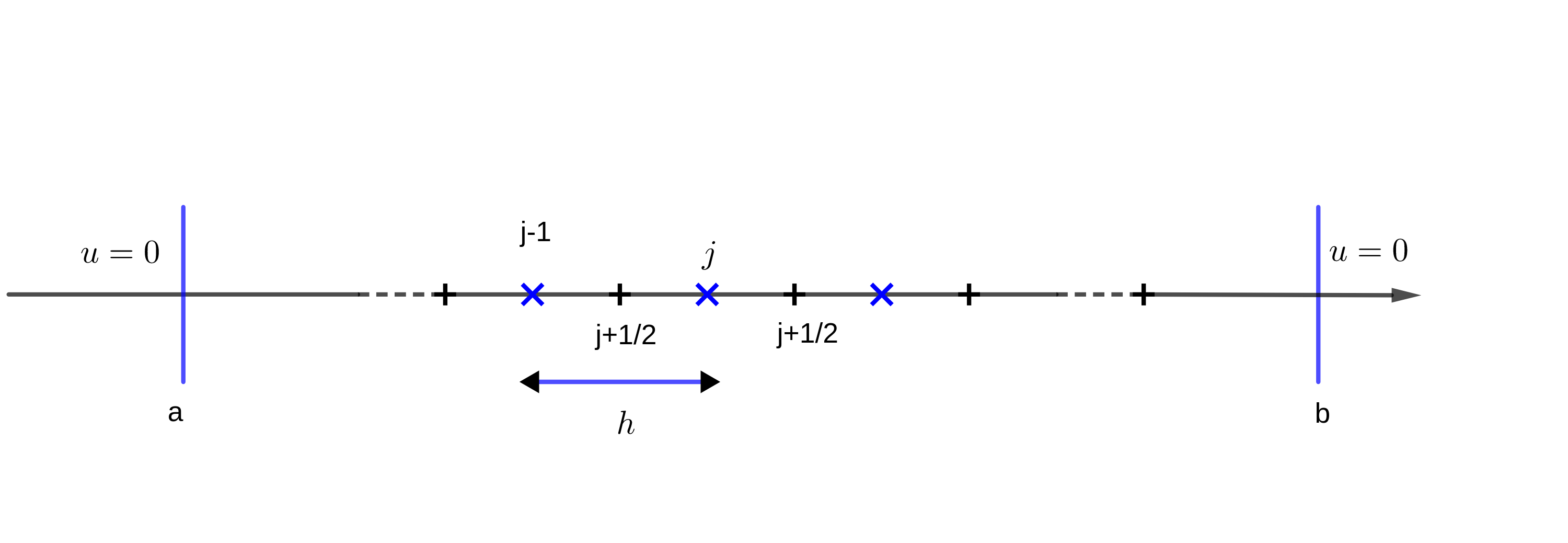
We use the trapezium rule to approximate the integral in the second equation of the system (5). We introduce a geometric grid on the $\xi$ axis, defined by the lower limit ${\xi }_m$, the upper limit ${\xi }_M$ and the number of discretisation points $N_{\xi }$. We note that:

$$\mathrm{\Delta }\xi =\frac{{\xi }_M-{\xi }_m}{N_{\xi }-1},$$

$${\int }_0^{+\mathrm{\infty }}\frac{\partial \phi }{\partial t}(x,t,\xi )𝑑M_{\alpha }(\xi )\simeq {\int }_{{\xi }_m}^{{\xi }_M}\frac{\partial \phi }{\partial t}(x,t,\xi )𝑑M_{\alpha }(\xi )\simeq \sum _{j=1}^{N_{\xi }}{w}_j\frac{\partial \phi }{\partial t}(x,t,{\xi }_j),$$

with

$$w_1=\frac{\sin (\alpha \pi )}{2\pi }{\xi }_m^{-\alpha }\mathrm{\Delta }\xi ,w_{N_{\xi }}=\frac{\sin (\alpha \pi )}{2\pi }{\xi }_M^{-\alpha }\mathrm{\Delta }\xi$$

and

$$w_j=\frac{\sin (\alpha \pi )}{\pi }{\xi }_j^{-\alpha }\mathrm{\Delta }\xi ,\forall j=2,\mathrm{\dots },N_{\xi }-1.$$

The system (5) then becomes:

(6a) $\rho \frac{{\partial }^{2}u}{\partial t^2}(x,t)-\frac{\partial \sigma }{\partial x}(x,t)=f(x,t),$

(6b) ${\tau }_0\frac{\partial s}{\partial t}(x,t)+{\displaystyle \sum _{j=1}^{N_{\xi }}}{w}_j\frac{\partial \phi }{\partial t}(x,t,{\xi }_j)=\mu ({\tau }_1-{\tau }_0)\frac{{\partial }^{2}u}{\partial x\partial t}(x,t),$

(6c) $\frac{\partial \phi }{\partial t}(x,t,{\xi }_j)=-{\xi }_j\phi (x,t,{\xi }_j)+s(x,t),j=1,\mathrm{\dots },N_{\xi },$

(6d) $\sigma (x,t)=s(x,t)+\mu \frac{\partial u}{\partial x}(x,t),$

(6e) $u(x,0)=u_0(x),\frac{\partial u}{\partial t}(x,0)=u_1(x),s(x,0)=0,\phi (x,0,{\xi }_j)=0,$

3.1. Space discretization

We introduce a regular mesh of the domain $\mathrm{\Omega }=[a,b]$ with edges $h=\frac{b-a}{N_x}$ consisting of the segments $[x_i,x_{i+1}],i=1,\mathrm{\dots },N_x$,

$$x_i=a+(i-1)h.$$

Figure 1. Space discretization.

We approach the equation (6a) in the point $x_i$ and the equation (6b), (6c) and (6d) in the point $x_{i+1/2}=(x_i+x_{i+1})/2$. We propose the centered scheme:

(7a) $\rho \frac{d^2{u}_i(t)}{d{t}^2}-\frac{{\sigma }_{i+\frac{1}{2}}(t)-{\sigma }_{i-\frac{1}{2}}(t)}{h}=f_i(t),$

(7b) ${\tau }_0\frac{d{s}_{i+\frac{1}{2}}(t)}{dt}+{\displaystyle \sum _{j=1}^{N_{\xi }}}{w}_j{\displaystyle \frac{d{\phi }_{i+\frac{1}{2},j}(t)}{dt}}=\mu ({\tau }_1-{\tau }_0)\left(\frac{d}{dt}\left(\frac{u_{i+1}(t)-u_i(t)}{h}\right)\right),$

(7c) $\frac{d{\phi }_{i+\frac{1}{2},j}(t)}{dt}=-{\xi }_j{\phi }_{i+\frac{1}{2},j}(t)+s_{i+\frac{1}{2}}(t),j=1,\mathrm{\dots },N_{\xi },$

(7d) ${\sigma }_{i+\frac{1}{2}}(t)=s_{i+\frac{1}{2}}(t)+\mu \frac{u_{i+1}(t)-u_i(t)}{h},$

(7e) $u_i(0)=u_0(x_i),\frac{d{u}_i}{dt}(0)=u_1(x_i),s_{i+\frac{1}{2}}(0)=0,{\phi }_{i+\frac{1}{2},j}(0)=0,$

with $u_i(t)\approx u(x_i,t)$, ${\sigma }_{i+\frac{1}{2}}(t)\approx \sigma (x_{i+1/2},t)$, $s_{i+\frac{1}{2}}(t)\approx s(x_{i+1/2},t)$, ${\phi }_{i+\frac{1}{2},j}(t)\approx \phi (x_{i+1/2},t,{\xi }_j)$ and $f_i(t)\approx f(x_i,t)$.

3.2. Space-time discretization

We consider a regular time grid with a step size of $\mathrm{\Delta }t$ and we set

$$t^n=n\mathrm{\Delta }t,t^{n+1/2}=t^n+\frac{\mathrm{\Delta }t}{2},\forall n.$$

In order to approximate the system (7), we use a centered finite difference scheme in time by approaching the first equation at $t^n$, the second and third equations at $t^{n+1/2}$, and the last equation at $t^n$. The resulting centred scheme is as follows:

(8a) $\rho \frac{u_i^{n+1}-2u_i^n+u_i^{n-1}}{\mathrm{\Delta }{t}^2}-\frac{{\sigma }_{i+\frac{1}{2}}^n-{\sigma }_{i-\frac{1}{2}}^n}{h}=f_i^n,$

(8b) ${\tau }_0\frac{s_{i+\frac{1}{2}}^{n+1}-s_{i+\frac{1}{2}}^n}{\mathrm{\Delta }t}+{\displaystyle \sum _{j=1}^{N_{\xi }}}{w}_j\frac{{\phi }_{i+\frac{1}{2},j}^{n+1}-{\phi }_{i+\frac{1}{2},j}^n}{\mathrm{\Delta }t}=$

(8c) $\frac{\mu ({\tau }_1-{\tau }_0)}{h}\left(\frac{u_{i+1}^{n+1}-u_{i+1}^n}{\mathrm{\Delta }t}-\frac{u_i^{n+1}-u_i^n}{\mathrm{\Delta }t}\right),$

(8d) $\frac{{\phi }_{i+\frac{1}{2},j}^{n+1}-{\phi }_{i+\frac{1}{2},j}^n}{\mathrm{\Delta }t}=-{\xi }_j\frac{{\phi }_{i+\frac{1}{2},j}^{n+1}+{\phi }_{i+\frac{1}{2},j}^n}{2}+\frac{s_{i+\frac{1}{2}}^{n+1}+s_{i+\frac{1}{2}}^n}{2},j=1,\mathrm{\dots },N_{\xi },$

(8e) ${\sigma }_{i+\frac{1}{2}}^n=s_{i+\frac{1}{2}}^n+\mu \frac{u_{i+1}^n-u_i^n}{h},$

(8f) $u_i^0=u_0(x_i),u_i^1=u_i^0+\mathrm{\Delta }t{u}_1(x_i)+\frac{\mathrm{\Delta }{t}^2}{2\rho }\left(f_i^0+\frac{{\sigma }_{i+\frac{1}{2}}^0-{\sigma }_{i-\frac{1}{2}}^0}{h}\right),$

(8g) $s_{i+\frac{1}{2}}^0=0,{\phi }_{i+1/2,j}^0=0,$

with $u_i^n\approx u(x_i,t^n)$, ${\sigma }_{i+\frac{1}{2}}^n\approx \sigma (x_{i+1/2},t^n)$, $s_{i+\frac{1}{2}}^n\approx s(x_{i+1/2},t^n)$, ${\phi }_{i+\frac{1}{2},j}^n\approx \phi (x_{i+1/2},t^n,{\xi }_j)$ and $f_i^n\approx f(x_i,t^n)$.

By using the equation (8d), we have

$${\phi }_{i+\frac{1}{2},j}^{n+1}=\frac{2-{\xi }_j\mathrm{\Delta }t}{2+{\xi }_j\mathrm{\Delta }t}{\phi }_{i+\frac{1}{2},j}^n+\frac{\mathrm{\Delta }t}{2+{\xi }_j\mathrm{\Delta }t}(s_{i+\frac{1}{2}}^{n+1}+s_{i+\frac{1}{2}}^n),$$

after injecting this last equality into (8b), we obtain:

$\rho \frac{u_i^{n+1}-2u_i^n+u_i^{n-1}}{\mathrm{\Delta }{t}^2}-\frac{{\sigma }_{i+\frac{1}{2}}^n-{\sigma }_{i-\frac{1}{2}}^n}{h}=f_i^n,$

${\tau }_0\frac{s_{i+\frac{1}{2}}^{n+1}-s_{i+\frac{1}{2}}^n}{\mathrm{\Delta }t}+\lambda (s_{i+\frac{1}{2}}^{n+1}+s_{i+\frac{1}{2}}^n)-{\displaystyle \sum _{j=1}^{N_{\xi }}}\widetilde{w_j}{\phi }_{i+\frac{1}{2},j}^n=\frac{\mu ({\tau }_1-{\tau }_0)}{h}\left(\frac{u_{i+1}^{n+1}-u_{i+1}^n}{\mathrm{\Delta }t}-\frac{u_i^{n+1}-u_i^n}{\mathrm{\Delta }t}\right),$

${\phi }_{i+\frac{1}{2},j}^{n+1}=\frac{2-{\xi }_j\mathrm{\Delta }t}{2+{\xi }_j\mathrm{\Delta }t}{\phi }_{i+\frac{1}{2},j}^n+\frac{\mathrm{\Delta }t}{2+{\xi }_j\mathrm{\Delta }t}(s_{i+\frac{1}{2}}^{n+1}+s_{i+\frac{1}{2}}^n),j=1,\mathrm{\dots },N_{\xi },$

${\sigma }_{i+\frac{1}{2}}^n=s_{i+\frac{1}{2}}^n+\mu \frac{u_{i+1}^n-u_i^n}{h},$

$u_i^0=u_0(x_i),u_i^1=u_i^0+\mathrm{\Delta }t{u}_1(x_i)+\frac{\mathrm{\Delta }{t}^2}{2\rho }\left(f_i^0+\frac{{\sigma }_{i+\frac{1}{2}}^0-{\sigma }_{i-\frac{1}{2}}^0}{h}\right),s_{i+\frac{1}{2}}^0=0,{\phi }_{i+1/2,j}^0=0,$

with

$$\widetilde{w_j}={\xi }_j{w}_j\frac{2}{2+{\xi }_j\mathrm{\Delta }t}\text{and}\lambda =\sum _{j=1}^{N_{\xi }}\frac{w_j}{2+{\xi }_j\mathrm{\Delta }t}.$$

Finally, we obtain the fully explicit scheme:

$u_i^{n+1}=\frac{\mathrm{\Delta }{t}^2}{\rho }\left(f_i^n+\frac{{\sigma }_{i+\frac{1}{2}}^n-{\sigma }_{i-\frac{1}{2}}^n}{h}\right)+2u_i^n-u_i^{n-1},$

$s_{i+\frac{1}{2}}^{n+1}=\frac{\mathrm{\Delta }t}{{\tau }_0+\lambda \mathrm{\Delta }t}\left(\frac{\mu ({\tau }_1-{\tau }_0)}{h}\left[\frac{u_{i+1}^{n+1}-u_{i+1}^n}{\mathrm{\Delta }t}-\frac{u_i^{n+1}-u_i^n}{\mathrm{\Delta }t}\right]+{\displaystyle \sum _{j=1}^{N_{\xi }}}\widetilde{w_j}{\phi }_{i+\frac{1}{2},j}^n\right)-\frac{\lambda \mathrm{\Delta }t-{\tau }_0}{\lambda \mathrm{\Delta }t+{\tau }_0}{s}_{i+\frac{1}{2}}^n,$

${\phi }_{i+\frac{1}{2},j}^{n+1}=\frac{2-{\xi }_j\mathrm{\Delta }t}{2+{\xi }_j\mathrm{\Delta }t}{\phi }_{i+\frac{1}{2},j}^n+\frac{\mathrm{\Delta }t}{2+{\xi }_j\mathrm{\Delta }t}\left(s_{i+\frac{1}{2}}^{n+1}+s_{i+\frac{1}{2}}^n\right),j=1,\mathrm{\dots },N_{\xi },$

${\sigma }_{i+\frac{1}{2}}^n=s_{i+\frac{1}{2}}^n+\mu \frac{u_{i+1}^n-u_i^n}{h},$

$u_i^0=u_0(x_i),u_i^1=u_i^0+\mathrm{\Delta }t{u}_1(x_i)+\frac{\mathrm{\Delta }{t}^2}{2\rho }\left(f_i^0+\frac{{\sigma }_{i+\frac{1}{2}}^0-{\sigma }_{i-\frac{1}{2}}^0}{h}\right),$

$s_{i+\frac{1}{2}}^0=0,{\phi }_{i+1/2,j}^0=0.$

We note that the number of unknowns can be reduced by replacing the expression for ${\sigma }_{i+\frac{1}{2}}^n$ in the first equation of the final system. This yields:

$u_i^{n+1}=$ $\frac{\mathrm{\Delta }{t}^2}{\rho }\left(f_i^n+\mu \frac{u_{i+1}^n-2u_i^n+u_{i-1}^n}{h^2}+\frac{s_{i+\frac{1}{2}}^n-s_{i-\frac{1}{2}}^n}{h}\right)+2u_i^n-u_i^{n-1},$

$s_{i+\frac{1}{2}}^{n+1}=$ $\frac{\mathrm{\Delta }t}{{\tau }_0+\lambda \mathrm{\Delta }t}\left(\frac{\mu ({\tau }_1-{\tau }_0)}{h}\left[\frac{u_{i+1}^{n+1}-u_{i+1}^n}{\mathrm{\Delta }t}-\frac{u_i^{n+1}-u_i^n}{\mathrm{\Delta }t}\right]+{\displaystyle \sum _{j=1}^{N_{\xi }}}\widetilde{w_j}{\phi }_{i+\frac{1}{2},j}^n\right)-\frac{\lambda \mathrm{\Delta }t-{\tau }_0}{\lambda \mathrm{\Delta }t+{\tau }_0}{s}_{i+\frac{1}{2}}^n,$

${\phi }_{i+\frac{1}{2},j}^{n+1}=$ $\frac{2-{\xi }_j\mathrm{\Delta }t}{2+{\xi }_j\mathrm{\Delta }t}{\phi }_{i+\frac{1}{2},j}^n+\frac{\mathrm{\Delta }t}{2+{\xi }_j\mathrm{\Delta }t}\left(s_{i+\frac{1}{2}}^{n+1}+s_{i+\frac{1}{2}}^n\right),j=1,\mathrm{\dots },N_{\xi },$

$u_i^0=$ $u_0(x_i),u_i^1=u_i^0+\mathrm{\Delta }t{u}_1(x_i)+\frac{\mathrm{\Delta }{t}^2}{\rho }\left(f_i^0+\frac{{\sigma }_{i+\frac{1}{2}}^0-{\sigma }_{i-\frac{1}{2}}^0}{h}\right),$

$s_{i+\frac{1}{2}}^0=$ $0,{\phi }_{i+1/2,j}^0=0.$

3.3. Discrete energy and stability analysis

We will use an energy technique to prove the stability of the scheme (see (3.2)). We introduce discrete normed spaces.

(9)

(10)

With the scalar products:

${(u_h,{\tilde{u}}_h)}_0$ $=h{\displaystyle \sum _i}{u}_i{\tilde{u}}_i,{({\sigma }_h,{\tilde{\sigma }}_h)}_{1/2}=h{\displaystyle \sum _i}{\sigma }_{i+1/2}{\tilde{\sigma }}_{i+1/2},{({\phi }_{h,j},{\tilde{\phi }}_{h,j})}_{1/2}$

$=h{\displaystyle \sum _i}{\phi }_{i+1/2,j}{\tilde{\phi }}_{i+1/2,j},j=1,\mathrm{\dots },N_{\xi },$

where

$$u_h={(u_i)}_{i\in \mathbb{Z}}\in L_{h,0}^2,{\sigma }_h={({\sigma }_{i+1/2})}_{i\in \mathbb{Z}}\in L_{h,1/2}^2$$

$${\phi }_{h,j}={({\phi }_{i+1/2,j})}_{i\in \mathbb{Z}}\in L_{h,1/2}^2,j=1,\mathrm{\dots },N_{\xi },$$

and associated norm:

${\Vert u_h\Vert }_0^2$ $=h{\displaystyle \sum _i}{\left|u_i\right|}^2,{\Vert {\sigma }_h\Vert }_{1/2}^2=h{\displaystyle \sum _i}{\left|{\sigma }_{i+1/2}\right|}^2,$

${\Vert {\phi }_{h,j}\Vert }_{1/2}^2$ $=h{\displaystyle \sum _i}{\left|{\phi }_{i+1/2,j}\right|}^2,j=1,\mathrm{\dots },N_{\xi }.$

We recall that the results for energy decay in the continuous case are given by (see [25]):

$E(t)=$ $\frac{1}{2}({\displaystyle {\int }_{ℝ}}\rho |\frac{\partial u}{\partial t}{|}^{2}dx+{\displaystyle {\int }_{ℝ}}\mu |\frac{\partial u}{\partial x}{|}^{2}dx+\frac{{\tau }_0}{\mu ({\tau }_1-{\tau }_0)}{\displaystyle {\int }_{ℝ}}|s{|}^{2}dx$

(11) $+\frac{1}{\mu ({\tau }_1-{\tau }_0)}{\displaystyle {\int }_{ℝ}}{\displaystyle {\int }_0^{+\mathrm{\infty }}}\xi |\phi {|}^{2}d{M}_{\alpha }(\xi )dx),$

and it satisfies:

$$\begin{array}{c}\frac{dE(t)}{dt}=(f,\frac{\partial u}{\partial t})-\frac{1}{\mu ({\tau }_1-{\tau }_0)}{\int }_{ℝ}{\int }_0^{+\mathrm{\infty }}{|s-\xi \phi |}^2𝑑M_{\alpha }(\xi )𝑑x,\end{array}$$

with

$$\begin{array}{c}s=\sigma -\mu \frac{\partial u}{\partial x}.\end{array}$$

We write the system (3.2) in vector form:

(12) $$\begin{array}{c}\rho \frac{u_h^{n+1}-2u_h^n+u_h^{n-1}}{\mathrm{\Delta }{t}^2}-B{\sigma }_h^n=0,\hfill \\ \frac{{\tau }_0}{\mu ({\tau }_1-{\tau }_0)}\frac{s_h^{n+1}-s_h^n}{\mathrm{\Delta }t}+\frac{1}{\mu ({\tau }_1-{\tau }_0)}\sum _{j=1}^{N_{\xi }}{w}_j\frac{{\phi }_{h,j}^{n+1}-{\phi }_{h,j}^n}{\mathrm{\Delta }t}+B^{\ast }\frac{u_h^{n+1}-u_h^n}{\mathrm{\Delta }t}=0,j=1,\mathrm{\dots },N_{\xi },\hfill \\ \frac{{\phi }_{h,j}^{n+1}-{\phi }_{h,j}^n}{\mathrm{\Delta }t}=-{\xi }_j\frac{{\phi }_{h,j}^{n+1}+{\phi }_{h,j}^n}{2}+\frac{s_h^{n+1}+s_h^n}{2},j=1,\mathrm{\dots },N_{\xi },\hfill \\ {\mu }^{-1}{\sigma }_h^n-{\mu }^{-1}{s}_h^n+B^{\ast }{u}_h^n=0.\hfill \end{array}$$

with

(13) $$\{\begin{array}{c}B:L_{h,1/2}^2⟶L_{h,0}^2\hfill \\ {\sigma }_h⟼{\left(\frac{{\sigma }_{i+1/2}-{\sigma }_{i-1/2}}{h}\right)}_{j\in \mathbb{Z}}\hfill \end{array}$$

Lemma 1.

The norm of the operator $B$ satisfies the inequality:

(14) $$\Vert B\Vert \le \frac{2}{h}.$$

Proof.

However, as ${\displaystyle \sum _{i\in 𝕫}}h{|u_{i+1}-u_i|}^2$ verifies the inequality:

it implies that

$$(B{\sigma }_h,u_h)\le \frac{2}{h}{\Vert u_h\Vert }_0{\Vert {\sigma }_h\Vert }_{1/2},$$

and we get

$$\Vert B\Vert \le \frac{2}{h}.$$

∎

Definition 2.

We define the discrete energy by:

$E^{n+1/2}=$ $\frac{\rho }{2}{\Vert \frac{u_h^{n+1}-u_h^n}{\mathrm{\Delta }t}\Vert }_0^2+\frac{\mu }{2}{(B^{\ast }{u}^{n+1},B^{\ast }{u}^n)}_0$

$+\frac{{\tau }_0}{4\mu ({\tau }_1-{\tau }_0)}\left[{\Vert s_h^{n+1}\Vert }_{1/2}^2+{\Vert s_h^n\Vert }_{1/2}^2\right]$

(15) $+\frac{\mathrm{\Delta }{t}^2}{4}{(B^{\ast }\frac{u_h^{n+1}-u_h^n}{\mathrm{\Delta }t},\frac{s_h^{n+1}-s_h^n}{\mathrm{\Delta }t})}_{1/2}$

$+\frac{1}{4\mu ({\tau }_1-{\tau }_0)}{\displaystyle \sum _{j=1}^{N_{\xi }}}{w}_j{\xi }_j\left[{\Vert {\phi }_{h,j}^{n+1}\Vert }_{1/2}^2+{\Vert {\phi }_{h,j}^n\Vert }_{1/2}^2\right].$

Remark 3.

The discrete energy can be decomposed as the sum of four terms.

• The first term, $\frac{\rho }{2}{\Vert \frac{u_h^{n+1}-u_h^n}{\mathrm{\Delta }t}\Vert }_0^2+\frac{1}{2}{(B^{\ast }{u}^{n+1},\mu B^{\ast }{u}^n)}_{1/2}$ corresponds to the classical discrete energy in the purely elastic case (i.e., when ${\tau }_0={\tau }_1=0$), which corresponds to the approximation of the first and second part of the continuous energy (3.3).

• The second term, $\frac{{\tau }_0}{4\mu ({\tau }_1-{\tau }_0)}\left[{\Vert s_h^{n+1}\Vert }_{1/2}^2+{\Vert s_h^n\Vert }_{1/2}^2\right]$ due to the viscoelasticity, which approaches the third parts of the continuous energy.

• The third term, $\frac{\mathrm{\Delta }{t}^2}{2}{(B^{\ast }\frac{u_h^{n+1}-u_h^n}{\mathrm{\Delta }t},\frac{s_h^{n+1}-s_h^n}{\mathrm{\Delta }t})}_{1/2}$ is a small term of order $𝒪(\mathrm{\Delta }{t}^2)$, which is due to the finite difference approximation.

• The last term, $\frac{1}{4\mu ({\tau }_1-{\tau }_0)}{\displaystyle \sum _{j=1}^{N_{\xi }}}{w}_j{\xi }_j\left[{\Vert {\phi }_{h,j}^{n+1}\Vert }_{1/2}^2+{\Vert {\phi }_{h,j}^n\Vert }_{1/2}^2\right]$ depends on $\alpha$ the fractional derivative order corresponds to the approximation of the last part of the continuous energy.

The following theorem proves an energy decay result.

Theorem 4.

The discrete energy verifies:

(16) $$\frac{E^{n+1/2}-E^{n-1/2}}{\mathrm{\Delta }t}=-\frac{1}{2\mu ({\tau }_1-{\tau }_0)}\sum _{j=1}^{N_{\xi }}{w}_j\left[{\Vert \frac{{\phi }_{h,j}^{n+1}-{\phi }_{h,j}^n}{\mathrm{\Delta }t}\Vert }_{1/2}^2+{\Vert \frac{{\phi }_{h,j}^n-{\phi }_{h,j}^{n-1}}{\mathrm{\Delta }t}\Vert }_{1/2}^2\right].$$

Proof.

We use the variational formulation associated with the discrete scheme (12):

$(\rho \frac{u_h^{n+1}-2u_h^n+u_h^{n-1}}{\mathrm{\Delta }{t}^2},{\tilde{u}}_h)-(B{\sigma }_h^n,{\tilde{u}}_h)=0,$

(17) $(\frac{{\tau }_0}{\mu ({\tau }_1-{\tau }_0)}\frac{s_h^{n+1}-s_h^n}{\mathrm{\Delta }t},{\tilde{s}}_h)+(\frac{1}{\mu ({\tau }_1-{\tau }_0)}{\displaystyle \sum _{j=1}^{N_{\xi }}}{w}_j\frac{{\phi }_{h,j}^{n+1}-{\phi }_{h,j}^n}{\mathrm{\Delta }t},{\tilde{s}}_h)+(B^{\ast }\frac{u_h^{n+1}-u_h^n}{\mathrm{\Delta }t},{\tilde{s}}_h)=0,$

$\frac{{\phi }_{h,j}^{n+1}-{\phi }_{h,j}^n}{\mathrm{\Delta }t}=-{\xi }_j\frac{{\phi }_{h,j}^{n+1}+{\phi }_{h,j}^n}{2}+\frac{s_h^{n+1}+s_h^n}{2},$

${\mu }^{-1}{\sigma }_h^n-{\mu }^{-1}{s}_h^n+B^{\ast }{u}_h^n=0.$

If we take ${\tilde{u}}_h=\frac{u_h^{n+1}-u_h^{n-1}}{2\mathrm{\Delta }t}$ (the centered approximation of $\frac{d{u}_h}{dt}$ in time $t^n$) and ${\tilde{s}}_h=\frac{s_h^{n+1}+s_h^n}{2}$ (the centered approximation of $s_h$ in time $t^{n+1/2}$). Equation (17) becomes:

(18)

Substituting $\frac{s_h^{n+1}+s_h^n}{2}$ into equation (3) and then into equation (2) gives:

(19)

which becomes:

(20) $$\begin{array}{c}i)(\rho \frac{u_h^{n+1}-2u_h^n+u_h^{n-1}}{\mathrm{\Delta }{t}^2},\frac{u_h^{n+1}-u_h^{n-1}}{2\mathrm{\Delta }t}){}_0-(B^{\ast }\frac{u_h^{n+1}-u_h^{n-1}}{2\mathrm{\Delta }t},{\sigma }_h^n){}_{1/2}=0,\hfill \\ ii)(\frac{{\tau }_0}{\mu ({\tau }_1-{\tau }_0)}\frac{s_h^{n+1}-s_h^n}{\mathrm{\Delta }t},\frac{s_h^{n+1}+s_h^n}{2}){}_{1/2}+(\frac{1}{\mu ({\tau }_1-{\tau }_0)}\sum _{j=1}^{N_{\xi }}{w}_j\frac{{\phi }_{h,j}^{n+1}-{\phi }_{h,j}^n}{\mathrm{\Delta }t},\frac{{\phi }_{h,j}^{n+1}-{\phi }_{h,j}^n}{\mathrm{\Delta }t}){}_{1/2}+\hfill \\ +{(\frac{1}{\mu ({\tau }_1-{\tau }_0)}\sum _{j=1}^{N_{\xi }}{w}_j\frac{{\phi }_{h,j}^{n+1}-{\phi }_{h,j}^n}{\mathrm{\Delta }t},{\xi }_j\frac{{\phi }_{h,j}^{n+1}+{\phi }_{h,j}^n}{2})}_{1/2}+{(B^{\ast }\frac{u_h^{n+1}-u_h^n}{\mathrm{\Delta }t},\frac{s_h^{n+1}+s_h^n}{2})}_{1/2}=0.\hfill \end{array}$$

We get:

$$i)\begin{array}{c}\frac{\rho }{2\mathrm{\Delta }t}\left[{\Vert \frac{u_h^{n+1}-u_h^n}{\mathrm{\Delta }t}\Vert }_0^2-{\Vert \frac{u_h^n-u_h^{n-1}}{\mathrm{\Delta }t}\Vert }_0^2\right]-{(B^{\ast }\frac{u_h^{n+1}-u_h^{n-1}}{2\mathrm{\Delta }t},{\sigma }_h^n)}_{1/2}=0.\hfill \end{array}$$

$$ii)\begin{array}{c}\frac{{\tau }_0}{2\mathrm{\Delta }t\mu ({\tau }_1-{\tau }_0)}\left[{\Vert s_h^{n+1}\Vert }_{1/2}^2-{\Vert s_h^n\Vert }_{1/2}^2\right]+\frac{1}{\mu ({\tau }_1-{\tau }_0)}\sum _{j=1}^{N_{\xi }}{w}_j{\Vert \frac{{\phi }_{h,j}^{n+1}-{\phi }_{h,j}^n}{\mathrm{\Delta }t}\Vert }_{1/2}^2+\hfill \\ +\frac{1}{2\mathrm{\Delta }t\mu ({\tau }_1-{\tau }_0)}\sum _{j=1}^{N_{\xi }}{w}_j{\xi }_j\left[{\Vert {\phi }_{h,j}^{n+1}\Vert }_{1/2}^2-{\Vert {\phi }_{h,j}^n\Vert }_{1/2}^2\right]+{(B^{\ast }\frac{u_h^{n+1}-u_h^n}{\mathrm{\Delta }t},\frac{s_h^{n+1}+s_h^n}{2})}_{1/2}=0.\hfill \end{array}$$

Using the last equation of (18), we obtain:

We use that ${\sigma }_h^n-s_h^n=-\mu B^{\ast }{u}_h^n$, which allows us to rewrite $(i)$ in the form:

(21) $$\begin{array}{c}\frac{\rho }{2\mathrm{\Delta }t}\left[{\Vert \frac{u_h^{n+1}-u_h^n}{\mathrm{\Delta }t}\Vert }_0^2-{\Vert \frac{u_h^n-u_h^{n-1}}{\mathrm{\Delta }t}\Vert }_0^2\right]+\hfill \\ +\frac{1}{2\mathrm{\Delta }t}\left[{(B^{\ast }{u}_h^{n+1},\mu B^{\ast }{u}_h^n)}_0-{(B^{\ast }{u}_h^{n-1},\mu B^{\ast }{u}_h^n)}_0\right]-{(B^{\ast }\frac{u_h^{n+1}-u_h^{n-1}}{2\mathrm{\Delta }t},s_h^n)}_{1/2}=0.\hfill \end{array}$$

If we average the equation $(ii)$ between the two moments $t^{n+\frac{1}{2}}$ and $t^{n-\frac{1}{2}}$, we obtain:

(22)

Equation (22) is equivalent to:

(23) $\frac{{\tau }_0}{4\mathrm{\Delta }t\mu ({\tau }_1-{\tau }_0)}\left[{\Vert s_h^{n+1}\Vert }_{1/2}^2+{\Vert s_h^n\Vert }_{1/2}^2\right]-\frac{{\tau }_0}{4\mathrm{\Delta }t\mu ({\tau }_1-{\tau }_0)}\left[{\Vert s_h^n\Vert }_{1/2}^2+{\Vert s_h^{n-1}\Vert }_{1/2}^2\right]$

$+\frac{1}{2\mu ({\tau }_1-{\tau }_0)}{\displaystyle \sum _{j=1}^{N_{\xi }}}{w}_j{\Vert \frac{{\phi }_{h,j}^{n+1}-{\phi }_{h,j}^n}{\mathrm{\Delta }t}\Vert }_{1/2}^2+\frac{1}{2\mu ({\tau }_1-{\tau }_0)}{\displaystyle \sum _{j=1}^{N_{\xi }}}{w}_j{\Vert \frac{{\phi }_{h,j}^n-{\phi }_{h,j}^{n-1}}{\mathrm{\Delta }t}\Vert }_{1/2}^2$

$+\frac{1}{4\mathrm{\Delta }t\mu ({\tau }_1-{\tau }_0)}{\displaystyle \sum _{j=1}^{N_{\xi }}}{w}_j{\xi }_j\left[{\Vert {\phi }_{h,j}^{n+1}\Vert }_{1/2}^2+{\Vert {\phi }_{h,j}^n\Vert }_{1/2}^2\right]$

$-\frac{1}{4\mathrm{\Delta }t\mu ({\tau }_1-{\tau }_0)}{\displaystyle \sum _{j=1}^{N_{\xi }}}{w}_j{\xi }_j\left[{\Vert {\phi }_{h,j}^n\Vert }_{1/2}^2+{\Vert {\phi }_{h,j}^{n-1}\Vert }_{1/2}^2\right]$

$+\frac{1}{2}{(B^{\ast }\frac{u_h^{n+1}-u_h^n}{\mathrm{\Delta }t},\frac{s_h^{n+1}+s_h^n}{2})}_{1/2}+\frac{1}{2}{(B^{\ast }\frac{u_h^n-u_h^{n-1}}{\mathrm{\Delta }t},\frac{s_h^n+s_h^{n-1}}{2})}_{1/2}$ $=0.$

We decompose the last two terms of this formula as follows:

(24) $$\begin{array}{c}\frac{1}{2}{(B^{\ast }\frac{u_h^{n+1}-u_h^n}{\mathrm{\Delta }t},\frac{s_h^{n+1}+s_h^n}{2})}_{1/2}=\frac{1}{2}{(B^{\ast }\frac{u_h^{n+1}-u_h^n}{\mathrm{\Delta }t},\frac{s_h^{n+1}-s_h^n}{2})}_{1/2}+\frac{1}{2}{(B^{\ast }\frac{u_h^{n+1}-u_h^n}{\mathrm{\Delta }t},s_h^n)}_{1/2}.\hfill \\ \frac{1}{2}{(B^{\ast }\frac{u_h^n-u_h^{n-1}}{\mathrm{\Delta }t},\frac{s_h^n+s_h^{n-1}}{2})}_{1/2}=-\frac{1}{2}{(B^{\ast }\frac{u_h^n-u_h^{n-1}}{\mathrm{\Delta }t},\frac{s_h^n-s_h^{n-1}}{2})}_{1/2}+\frac{1}{2}{(B^{\ast }\frac{u_h^n-u_h^{n-1}}{\mathrm{\Delta }t},s_h^n)}_{1/2}.\hfill \end{array}$$

Substitute (24) in (23), we get

(25) $$\begin{array}{c}-{(B^{\ast }\frac{u_h^{n+1}-u_h^{n-1}}{2\mathrm{\Delta }t},s_h^n)}_{1/2}=\frac{1}{2\mathrm{\Delta }t}\left(T_1^{n+1/2}-T_1^{n-1/2}\right)+\frac{1}{2\mathrm{\Delta }t}\left(T_2^{n+1/2}-T_2^{n-1/2}\right)\hfill \\ +\frac{1}{4\mathrm{\Delta }t}\left(T_3^{n+1/2}-T_3^{n-1/2}\right)+T^n,\hfill \end{array}$$

with

$T_1^{n+1/2}=$ $\frac{{\tau }_0}{2\mu ({\tau }_1-{\tau }_0)}\left[{\Vert s_h^{n+1}\Vert }_{1/2}^2+{\Vert s_h^n\Vert }_{1/2}^2\right],$

$T_2^{n+1/2}=$ $\frac{1}{2}{(B^{\ast }{u}_h^{n+1}-u_h^n,s_h^{n+1}-s_h^n)}_{1/2},$

$T_3^{n+1/2}=$ $\frac{1}{2\mu ({\tau }_1-{\tau }_0)}{\displaystyle \sum _{j=1}^{N_{\xi }}}{w}_j{\xi }_j\left[{\Vert {\phi }_{h,j}^{n+1}\Vert }_{1/2}^2+{\Vert {\phi }_{h,j}^n\Vert }_{1/2}^2\right],$

$T^n=$ $\frac{1}{2\mu ({\tau }_1-{\tau }_0)}{\displaystyle \sum _{j=1}^{N_{\xi }}}{w}_j{\Vert \frac{{\phi }_{h,j}^{n+1}-{\phi }_{h,j}^n}{\mathrm{\Delta }t}\Vert }_{1/2}^2+\frac{1}{2\mu ({\tau }_1-{\tau }_0)}{\displaystyle \sum _{j=1}^{N_{\xi }}}{w}_j{\Vert \frac{{\phi }_{h,j}^n-{\phi }_{h,j}^{n-1}}{\mathrm{\Delta }t}\Vert }_{1/2}^2\ge 0.$

After substitution of the quantity (25) in (21), we will find (4):

$$\frac{E^{n+1/2}-E^{n-1/2}}{\mathrm{\Delta }t}=-T^n\le 0,$$

which is the desired identity. ∎

Thanks to Theorem 4, in order to establish a sufficient stability condition it suffices to show that the energy $E^{n+1/2}$ is a positive quadratic form (see [26]). The same condition applies as in the integer derivative model discussed in [1] because the final term in the energy $E^{n+1/2}$ does not affect the positivity of the form.

Theorem 5.

The numerical scheme (12) is $L^2$ stable under the sufficient CFL condition:

(26) $$\mathrm{\Delta }t\le \frac{1}{c_{\mathrm{\infty }}}h,$$

where $c_{\mathrm{\infty }}=c\sqrt{\frac{{\tau }_1}{{\tau }_0}}$, which corresponds to the velocity of viscolastic wave s in height frequency and $c=\sqrt{\frac{\mu }{\rho }}$, which corresponds to the velocity of viscolastic waves in low frequency.

Proof.

We look for a condition in which the discrete energy is positive. To achieve this, we use the equivalent vector form of $E^{n+1/2}$:

(27)

As the following quantities verify:

$$\{\begin{array}{c}{\Vert s_h^{n+1}\Vert }_{1/2}^2+{\Vert s_h^n\Vert }_{1/2}^2=\frac{1}{2}\left({\Vert s_h^{n+1}+s_h^n\Vert }_{1/2}^2+{\Vert s_h^{n+1}-s_h^n\Vert }_{12}^2\right)\hfill \\ {(B^{\ast }{u}_h^{n+1},B^{\ast }{u}_h^n)}_0=\frac{1}{4}{\Vert B^{\ast }(u_h^{n+1}+u_h^n)\Vert }_0^2-\frac{1}{4}{\Vert B^{\ast }(u_h^{n+1}-u_h^n)\Vert }_0^2,\hfill \end{array}$$

we can rewrite $E^{n+1/2}$ in the form: $E^{n+1/2}=E_1^{n+1/2}+E_2^{n+1/2}$, where

$E_1^{n+1/2}=$ $\frac{\mu }{8}{\Vert B^{\ast }\frac{u_h^{n+1}+u_h^n}{2}\Vert }_0^2$

$+\frac{1}{4\mu ({\tau }_1-{\tau }_0)}\left(\frac{{\tau }_0}{2}{\Vert \frac{s_h^{n+1}+s_h^n}{2}\Vert }_{1/2}^2+{\displaystyle \sum _{j=1}^{N_{\xi }}}{w}_j{\xi }_j\left[{\Vert {\phi }_{h,j}^{n+1}\Vert }_{1/2}^2+{\Vert {\phi }_{h,j}^n\Vert }_{1/2}^2\right]\right)⩾0.$

${𝑬}_2^{n+1/2}=$ $\frac{\rho }{2}{\Vert \frac{u_h^{n+1}-u_h^n}{\mathrm{\Delta }t}\Vert }_0^2-\frac{\mu \mathrm{\Delta }{t}^2}{8}{\Vert B^{\ast }\frac{u_h^{n+1}-u_h^n}{\mathrm{\Delta }t}\Vert }_0^2+\frac{{\tau }_0}{\mu ({\tau }_1-{\tau }_0)}\frac{\mathrm{\Delta }{t}^2}{8}{\Vert \frac{s_h^{n+1}-s_h^n}{\mathrm{\Delta }t}\Vert }_{1/2}^2$

$+\frac{\mathrm{\Delta }{t}^2}{4}{(B^{\ast }\frac{u_h^{n+1}-u_h^n}{\mathrm{\Delta }t},\frac{s_h^{n+1}-s_h^n}{\mathrm{\Delta }t})}_{1/2}.$

Moreover, the quantity $E_2^{n+1/2}$ satisfies

${𝑬}_2^{n+1/2}⩾$

$⩾$ $\frac{1}{2}(\left[\rho I-\frac{\mu \mathrm{\Delta }{t}^2}{4}B{B}^{\ast }\right]\frac{u_h^{n+1}-u_h^n}{\mathrm{\Delta }t},\frac{u_h^{n+1}-u_h^n}{\mathrm{\Delta }t})+\frac{{\tau }_0}{\mu ({\tau }_1-{\tau }_0)}\frac{\mathrm{\Delta }{t}^2}{8}{\Vert \frac{s_h^{n+1}-s_h^n}{\mathrm{\Delta }t}\Vert }_{1/2}^2$

$-\frac{\mu ({\tau }_1-{\tau }_0)}{{\tau }_0}\frac{\mathrm{\Delta }{t}^2}{8}{(B{B}^{\ast }\frac{u_h^{n+1}-u_h^n}{\mathrm{\Delta }t},\frac{u_h^{n+1}-u_h^n}{\mathrm{\Delta }t})}_0-\frac{{\tau }_0}{\mu ({\tau }_1-{\tau }_0)}\frac{\mathrm{\Delta }{t}^2}{8}{\Vert \frac{s_h^{n+1}-s_h^n}{\mathrm{\Delta }t}\Vert }_{1/2}^2,$

$=$ $\frac{1}{2}(\rho \frac{u_h^{n+1}-u_h^n}{\mathrm{\Delta }t},\frac{u_h^{n+1}-u_h^n}{\mathrm{\Delta }t})-\left(\mu +\frac{\mu ({\tau }_1-{\tau }_0)}{{\tau }_0}\right)\frac{\mathrm{\Delta }{t}^2}{8}(B{B}^{\ast }\frac{u_h^{n+1}-u_h^n}{\mathrm{\Delta }t},\frac{u_h^{n+1}-u_h^n}{\mathrm{\Delta }t}),$

$=$ $\frac{1}{2}(\rho \frac{u_h^{n+1}-u_h^n}{\mathrm{\Delta }t},\frac{u_h^{n+1}-u_h^n}{\mathrm{\Delta }t})-\frac{\mu {\tau }_1}{{\tau }_0}\frac{\mathrm{\Delta }{t}^2}{8}(B{B}^{\ast }\frac{u_h^{n+1}-u_h^n}{\mathrm{\Delta }t},\frac{u_h^{n+1}-u_h^n}{\mathrm{\Delta }t}).$

The positivity of $E^{n+1/2}$ is ensured under the inequality

$$\frac{\mu {\tau }_1}{{\tau }_0}\frac{\mathrm{\Delta }{t}^2}{4}{(B{B}^{\ast }{u}_h,u_h)}_0⩽{(\rho u_h,u_h)}_0,\forall u_h.$$

this is equivalent to:

${\left(\sqrt{\frac{\mu {\tau }_1}{{\tau }_0}}\frac{\mathrm{\Delta }t}{2}\right)}^2{(B{u}_h,B{u}_h)}_0⩽$ ${(\rho u_h,u_h)}_0,\forall u_h,$

${\left(\sqrt{\frac{\mu {\tau }_1}{{\tau }_0}}\frac{\mathrm{\Delta }t}{2}\right)}^2{\Vert B\Vert }^2{\Vert u_h\Vert }_0^2⩽$ $\rho {\Vert u_h\Vert }_0^2,$

${\left(\sqrt{\frac{\mu {\tau }_1}{{\tau }_0}}\frac{\mathrm{\Delta }t}{2}\right)}^2{\Vert B\Vert }^2⩽$ $\rho ,$

we use Lemma 1, we get the stability sufficient condition:

$$\mathrm{\Delta }t\le h/c_{\mathrm{\infty }},\text{with}{c}_{\mathrm{\infty }}=c\sqrt{\frac{{\tau }_1}{{\tau }_0}}\text{ and }c=\sqrt{\frac{\mu }{\rho }}.$$

∎

Remark 6.

We observe that:

• The stability condition (26) is also necessary. Indeed, if we set $\mathrm{\Delta }t=\frac{h}{c_{\mathrm{\infty }}}(1+{10}^{-3})$ the numerical scheme will be unstable.

4. Numerical simulation

We validate the numerical scheme suggested in the previous section, since we have an exact solution for a particular choice of initial conditions. We consider the model problem in the segment $]0,1[$ with the following data:

(28)

and the coefficients:

$$\begin{array}{c}\rho =1,\mu =1,{\tau }_0=1,{\tau }_1=1.2.\end{array}$$

The exact solution $(u,\sigma )$ of the problem:

(29) $$\{\begin{array}{cc}u(x,t)=U(t)\sin (\pi x),\hfill & \\ \sigma (x,t)=\mathrm{\Sigma }(t)\pi \cos (\pi x).\hfill & \end{array}$$

Substituting (29) in (28) we find $U$ is solution of:

(30) $$\begin{array}{cc}\frac{d^{\alpha +2}U}{d{t}^{\alpha +2}}+\frac{dU}{dt}+{\pi }^2{\tau }_1\frac{d^{\alpha }U}{d{t}^{\alpha }}+{\pi }^{2}U=0\hfill & \\ U(0)=1,\frac{dU(0)}{dt}=0.\hfill & \end{array}$$

The solution of this system is of the form:

$U(t)=e^{\eta t}(\cos (\omega t)-\frac{\eta }{\omega }\sin (\omega t)),$

where $\eta \mp i\omega$ is the solution of:

$X^{\alpha +2}+X^2+{\tau }_1{\pi }^2{X}^{\alpha }+{\pi }^2=0,$

For the computation of the numerical solution, we use $h=0.1$ and ensure that the stability condition ($\mathrm{\Delta }t=h/c_{\mathrm{\infty }}$) is satisfied.

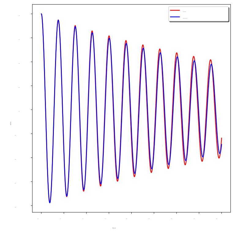
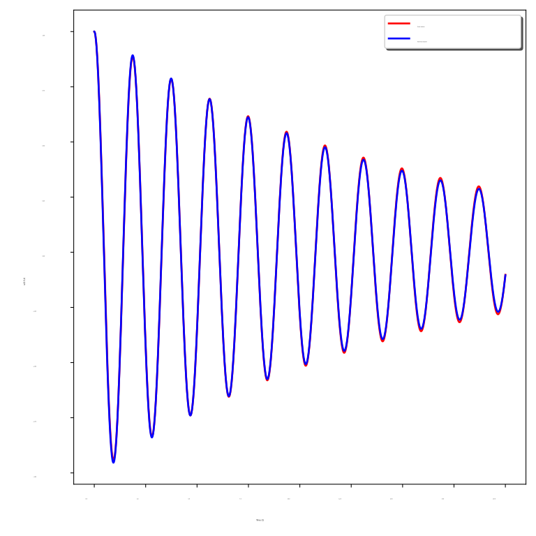
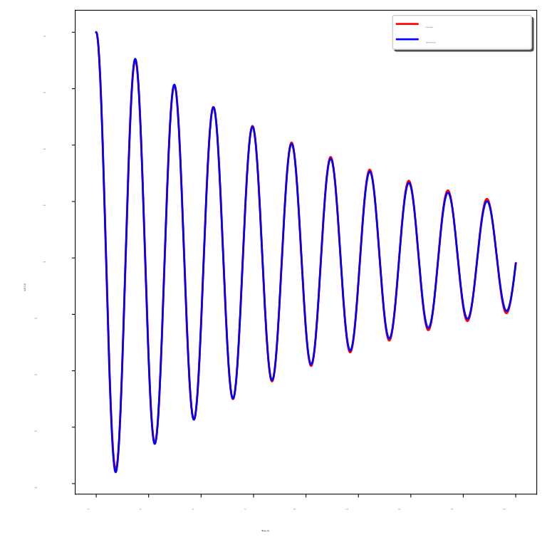
Fig. 2 shows a comparison of the exact solution ($u_{ex}$) and the numerical solution ($u_{num}$) at the point $x=0.5$ as a function of time for different values of $\alpha$.

$\alpha =0.3$	$\alpha =0.6$
$\alpha =0.7$	$\alpha =0.9$

Figure 2. The numerical and the exact solutions as a function of time for different $\alpha$.

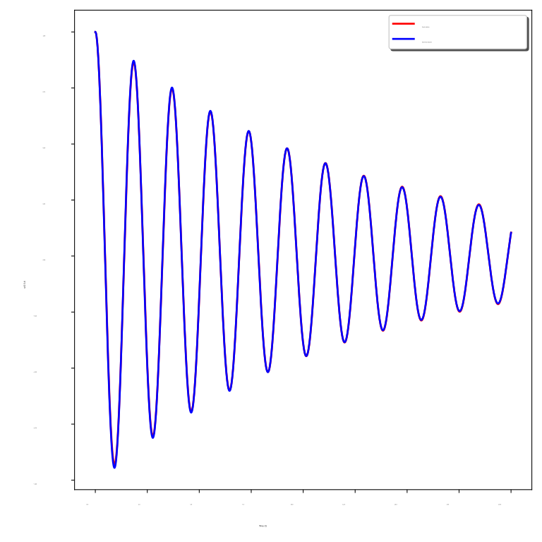We observe that the numerical solution coincides with the exact solution for all values of $\alpha$. The figure also shows that, for a large value of $\alpha$, the waves are more damped.

Numerical stability: The stability condition is given by $CFL=\frac{1}{c_{\mathrm{\infty }}}=\frac{1}{c\sqrt{{\tau }_1/{\tau }_0}}$, $c_{\mathrm{\infty }}$, where $c$ denotes the velocity of a high-frequency wave and $CFL$ is the Courant–Friedrichs–Lewy number.

For numerical stability, if we perturb the stability condition to be $CFL+{10}^{-5}$ and even by changing the value of $\alpha$, we will still have Fig. 3:

Figure 3. The numerical solution as a function of time following the perturbation is stability ${10}^{-5}$.

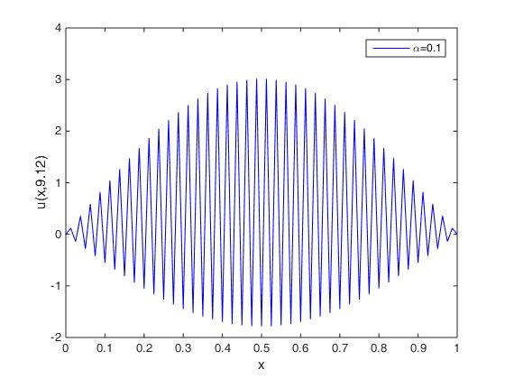
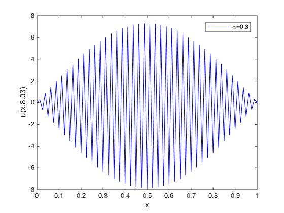
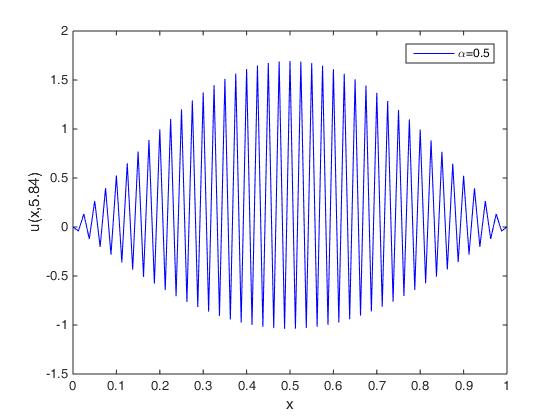
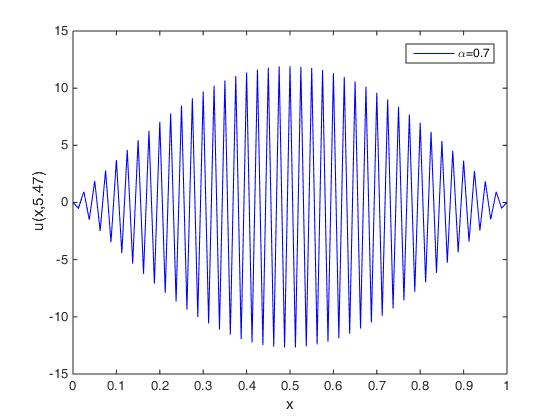
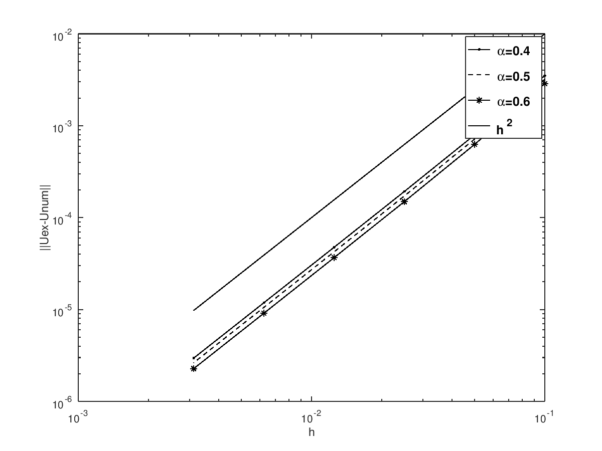
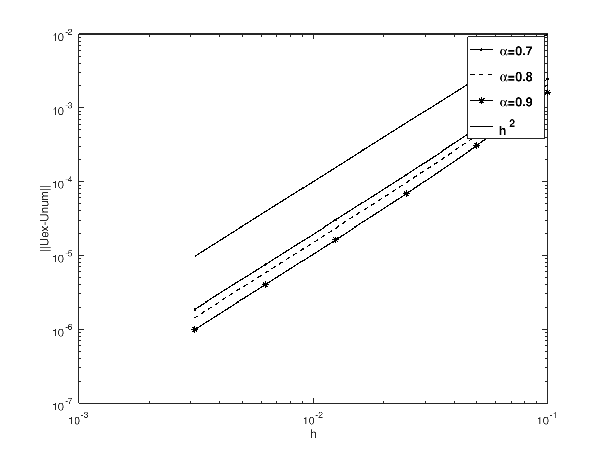
Fig. 4 shows the evolution of the numerical error, ${\Vert u_{exa}-u_{num}\Vert }_{\mathrm{\infty }}$ as a function of step h for two values of the parameter $\alpha$, namely $\alpha =0.5$ (left-hand panel) and $\alpha =0.9$ (right-hand panel).

$h$	${\Vert u_{exa}-u_{num}\Vert }_{\mathrm{\infty }}$
${10}^{-1}$	${\mathrm{3.2083\hspace{0.33em}10}}^{-03}$
${\mathrm{5\hspace{0.33em}10}}^{-2}$	${\mathrm{7.1497\hspace{0.33em}10}}^{-04}$
${\mathrm{2.5\hspace{0.33em}10}}^{-2}$	${\mathrm{1.7204\hspace{0.33em}10}}^{-04}$
${\mathrm{1.25\hspace{0.33em}10}}^{-2}$	${\mathrm{4.2436\hspace{0.33em}10}}^{-05}$
${\mathrm{6.25\hspace{0.33em}10}}^{-3}$	${\mathrm{1.0553\hspace{0.33em}10}}^{-05}$
${\mathrm{3.125\hspace{0.33em}10}}^{-3}$	${\mathrm{2.6326\hspace{0.33em}10}}^{-06}$

$h$	${\Vert u_{exa}-u_{num}\Vert }_{\mathrm{\infty }}$
${10}^{-1}$	${\mathrm{1.629\hspace{0.33em}10}}^{-03}$
${\mathrm{5\hspace{0.33em}10}}^{-2}$	${\mathrm{3.0609\hspace{0.33em}10}}^{-04}$
${\mathrm{2.5\hspace{0.33em}10}}^{-2}$	${\mathrm{6.8340\hspace{0.33em}10}}^{-05}$
${\mathrm{1.25\hspace{0.33em}10}}^{-2}$	${\mathrm{1.6344\hspace{0.33em}10}}^{-05}$
${\mathrm{6.25\hspace{0.33em}10}}^{-3}$	${\mathrm{4.01139\hspace{0.33em}10}}^{-06}$
${\mathrm{3.125\hspace{0.33em}10}}^{-3}$	${\mathrm{9.94608\hspace{0.33em}10}}^{-07}$

Figure 4. Error for $\alpha =0.5$ and $\alpha =0.9$.

We observe that the error decreases steadily as $h$ decreases, and that for the same step, the error is smaller when $alpha$ is larger.

To study the convergence of our scheme, we change the discretisation parameters h with $\mathrm{\Delta }t=\frac{h}{c_{\mathrm{\infty }}}$. Fig. 6 shows the $L^{\mathrm{\infty }}$-norm of the corresponding error with respect to the space step $h$ (on a log-log scale). Fig. 5–Fig. 6 shows that there is convergence and that the error is of order 2, regardless of the values of $\alpha$.

Figure 5. Convergence for value of $\alpha =0.4;\mathrm{\hspace{0.33em}0.5};\mathrm{\hspace{0.33em}0.6}$.

Figure 6. Convergence for value of $\alpha =0.7;\mathrm{\hspace{0.33em}0.8};\mathrm{\hspace{0.33em}0.9}$.

We conduct an experiment in the domain $[-5,5]$ with a point source located at the centre of the domain and verify:

$$t_0=\frac{1}{f_0},f_0=1\text{ central frequency },$$

with the following data:

$$u(x,0)=0,u_t(x,0)=0,\sigma (x,0)=0,x\in ]-5,5[,$$

$$u(-5,t)=u(5,t)=0,t\in [0,T],$$

and the coefficients:

$$\begin{array}{c}\rho =1,\mu =1.\end{array}$$

The parameters of the discretization are $h={5.10}^{-2}$ and $\mathrm{\Delta }t=\frac{h}{c_{\mathrm{\infty }}}$ satisfies the stability condition (26).

To demonstrate the impact of relaxation parameters, such as ${\tau }_0$ and ${\tau }_1$, on the attenuation and propagation velocity of fractional viscoelastic waves, we present a numerical solution in Fig. 7, where we vary the ratio, $\theta ={\tau }_1/{\tau }_0$, with values of: $4$, $2$ and $1.2$.

Figure 7. Damping and propagation quality with $\alpha =0.8$.

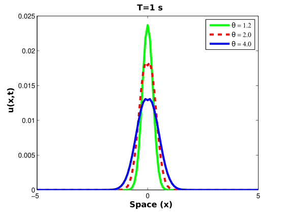
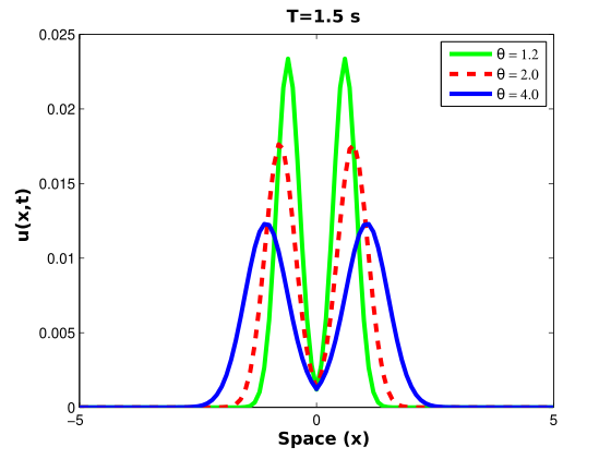
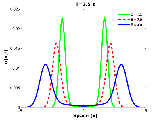
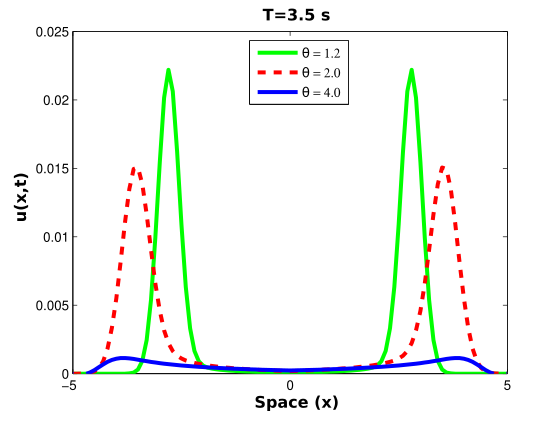
We can see that absorption and velocity of propagation are related to the ratio $\theta$: the larger the value of $\theta$, the greater the damping and the faster the velocity of propagation.

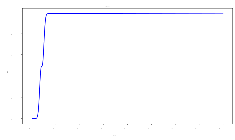
Fig. 8 shows that, after the source $f$ is extinguished, the viscoelastic energy decreases exponentially, which confirms our predictions (see (4)).

Figure 8. Discrete energy with $\theta =1.2$ and $\alpha =0.5$.

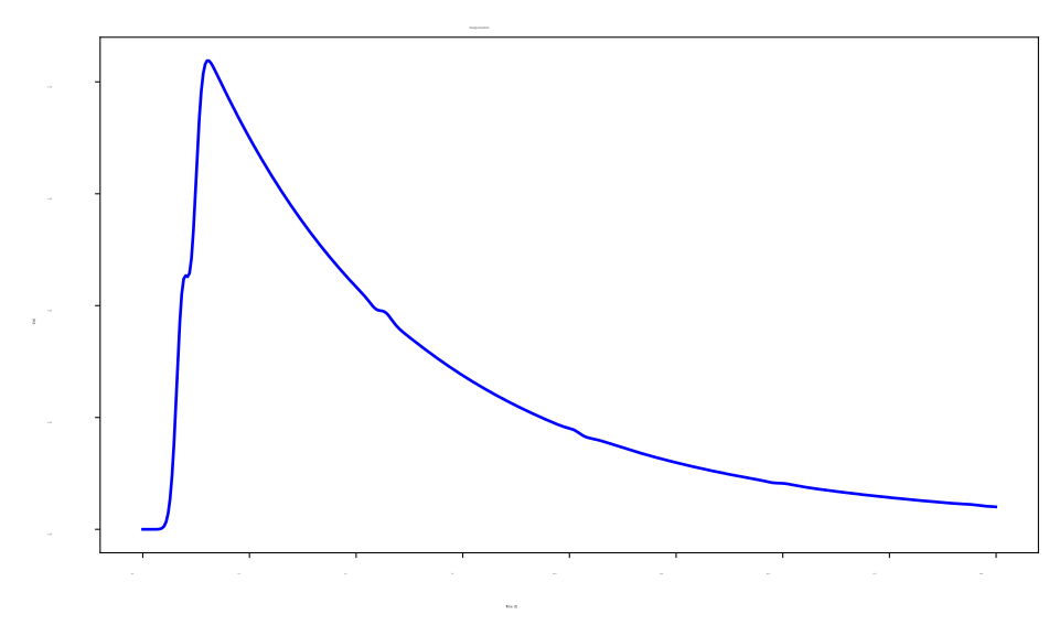
Fig. 9 shows the influence of the ratio $\theta$ on the discrete energy.

$\theta =1.8$	$\theta \approx 1$

Figure 9. Discrete energy with $\alpha =0.5$.

We observe that, when $\theta =1.8$, the discrete energy converges more quickly to zero. However, when $\theta =1.0001$ ($\theta \approx 1$), energy conservation occurs and the viscoelastic model converges to the elastic one.

4.1. Parameter Selection for Diffusive Representation

The diffusive representation introduces a continuous variable, denoted by the symbol $\xi$, which must be discretised over the interval $[{\xi }_m,{\xi }_M]$ with $N_{\xi }$ points. Through systematic numerical experimentation (see Fig. 10), we determine the optimal parameter ranges.

• ${\xi }_m\approx 0.01/T$ (characteristic timescale)

• ${\xi }_M\approx 10/\mathrm{\Delta }t$ (inverse time step)

• $N_{\xi }=50$-$100$ points (logarithmic spacing)

Figure 10. Sensitivity analysis showing the effect of (a) ${\xi }_m$, (b) ${\xi }_M$, and (c) $N_{\xi }$ on solution accuracy. Errors plateau when ${\xi }_m\le {10}^{-2}$, ${\xi }_M\ge {10}^3$, and $N_{\xi }\ge 50$.

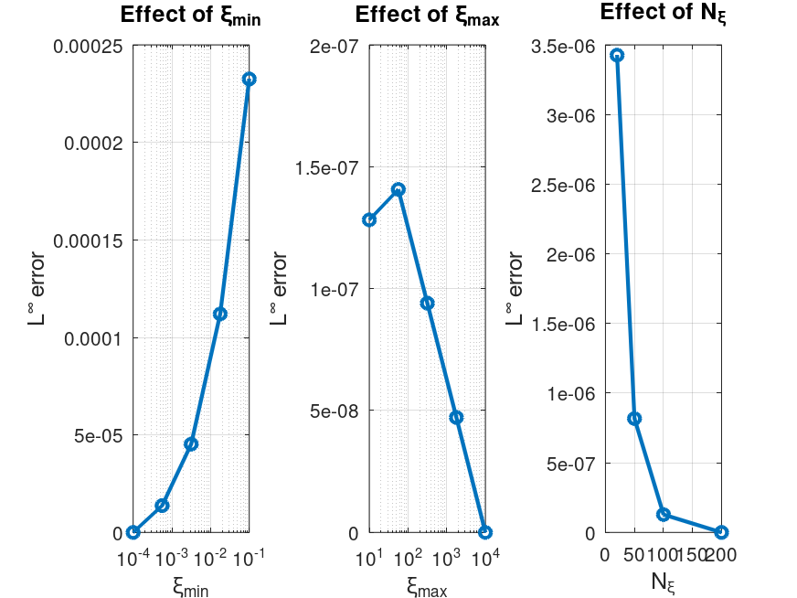
Fig. 10 illustrates the effect that diffusive scheme parameters have on the accuracy of the solution, as measured by the relative $L_{\mathrm{\infty }}$ error. Three clear trends emerge.

1. Sensitivity to ${\xi }_{\mathrm{m}}$ (see Fig. 10. on the left):

   • Error decreases exponentially as ${\xi }_{\mathrm{m}}\to 0$.

   • Stabilises for ${\xi }_{\mathrm{m}}\le {10}^{-2}$ (error ).

   • Confirms that the slow dynamics must be captured by the value of the parameter.

2. Influence of ${\xi }_M$ (middle figure in Fig. 10):

   • High-frequency truncation: Errors exceed ${10}^{-2}$ when due to loss of spectral resolution in the fractional kernel $t^{-\alpha }$

   • Convergence threshold: Numerical convergence (error ) is achieved for ${\xi }_M\ge {10}^3/\mathrm{\Delta }t$, where $\mathrm{\Delta }t$ is the time step

   • Optimal choice: Our selection ${\xi }_M={10}^3/\mathrm{\Delta }t$ ensures:

     (31)

3. Effect of $N_{\xi }$ (see Fig 10. on the right):

   • Spectral convergence is typical of fractional methods.

   • Negligible gain beyond 50 $N_{\xi }$points.

   • An error platform at approximately $5\times {10}^{-5}$.

5. Conclusion

In this study, we developed and analysed a second-order, explicit, finite-difference scheme for a fractional wave propagation model. Using energy methods, we derived a stability condition that is consistent with the classical (integer-order) case. Our analysis yielded a criterion that is both theoretically sufficient and numerically precise. A variety of numerical experiments demonstrated the impact of the fractional order $\alpha$ and the relaxation parameters ${\tau }_0$ and ${\tau }_1$ on wave attenuation. Future work will focus on extending the method to higher dimensions and improving the efficiency of adaptive time-stepping schemes. Furthermore, this approach can be applied to more complex models in poroelastic media, in which fractional effects are crucial for capturing memory and dissipation phenomena.

Data Availability

No data were used to support this study.