A simplified homotopy perturbation method
for nonlinear ill-posed operator equations
in Hilbert spaces

Abstract.

One popular regularization technique for handling both linear and nonlinear ill-posed problems is Homotopy perturbation. In order to solve nonlinear ill-posed problems, we investigate an iteratively-regularized simplified version of the Homotopy perturbation approach in this study. We examine the method’s thorough convergence analysis under typical circumstances, focusing on the nonlinearity and the convergence rate under a Hölder-type source condition. Lastly, numerical simulations are run to confirm the method’s effectiveness.

1. Introduction

There are numerous scientific and engineering applications that can lead to inverse problems. When inverse issues are formulated mathematically, they typically result in ill-posedness in the sense of Hadamard. Therefore, to find a stable approximation solution for the inverse issue, the regularization method is necessary. Numerous regularization techniques, including the Gauss-Newton iterative approach, the Thikhonov method, the Levrentiv iterative method, and the Levenberg Marquardt method, have been developed in the literature to address issues of this nature in Hilbert spaces (see, for example, [2], [3], [6], [10], [12], [16], [17], and [18]). One of the most popular iterative techniques for resolving nonlinear ill-posed problems in Hilbert spaces is the Landweber technique (cf. [4], [8], [11], [21], and [22]). Compared to other regularization techniques, this one is simpler to implement. A detailed explanation of this technique for the linear case can be found in [5].

In order to comprehend this approach, let us look at the abstract operator equation

(1) $$F(x)=y,$$

In this equation, $F:D(F)\subseteq X\to Y$ is a nonlinear operator on $D(F)$, and $X$ and $Y$ are Hilbert spaces with inner product $⟨.,.⟩$ and norm $\parallel .\parallel$ respectively. These operators can always be recognized by their context. $F^{\prime }(x)$ represents the Fréchet derivative of $F$ at $x$. Assume for the moment that $x^{†}$ is the exact solution (which does not need to be unique) to (1.1). We are mainly interested in problems of the form (1) for which the solution $x^{†}$ does not depend continuously on the data $y$. In real-world applications, precise data might not be accessible. Therefore, instead of using the actual data $y$, we use the available perturbed data with

(2) $$\Vert y^{\delta }-y\Vert \le \delta ,$$

where $\delta >0$ is the noise level.

Given that $F$ is locally scaled and Fréchet differentiable, let

(3) $$\Vert F^{\prime }(x)\Vert \le 1,\forall x\in B_{\rho }(x_0),$$

where $x_0$ is the initial guess for the exact solution and $\rho >0$. Next, Hanke et al. [8] examined the standard Landweber iteration for the non-linear case, which is as follows:

(4) $$x_{n+1}^{\delta }=x_n^{\delta }-F^{\prime }{(x_n^{\delta })}^{\ast }(F(x_n^{\delta })-y^{\delta }),$$

where $F^{\prime }{(x)}^{\ast }$ indicates the adjoint of the Fréchet derivative $F^{\prime }(x)$ for $x\in B_{\rho }(x_0)$, and $x_0$ is the initial guess for the exact solution. To examine technique (4), they took into account the following tangential type nonlinearity condition: With and $x,x^{\prime }\in B_{\rho }(x_0)\subset D(F)$,

(5) $$\Vert F(x)-F(x^{\prime })-F^{\prime }(x)(x-x^{\prime })\Vert \le \eta \Vert F(x)-F(x^{\prime })\Vert .$$

The method’s convergence analysis was conducted with the condition (5). For $0\le n\le n_{\delta }$, the iteration is terminated at $n_{\delta }$ by the generalised discrepancy principle

(6)

where $\tau >2\frac{1+\eta }{1-2\eta }>2$ is the positive constant dependent on $\eta$. Under the subsequent Hölder-type source condition, they were able to determine the rate of convergence:

(7)

To determine the rate of convergence for the approach (4), they also needed the following features of $F$, as the assumption (7) is insufficient:

(8) $$F^{\prime }(x)=R_x^{x^{\prime }}F(x^{\prime }),x,x^{\prime }\in B_{\rho }(x_0),$$

where $\{R_x^{x^{\prime }}:x,x^{\prime }\in B_{\rho }(x_0)\}$ is the family of bounded linear operators $R_x^{x^{\prime }}:Y\to Y$ such that

(9) $$\Vert R_x^{x^{\prime }}-I\Vert \le \text{C}\Vert x-x^{\prime }\Vert ,$$

where C is a positive constant.

Li Cao, Bo Han, and Wei Wang initially created homotopy perturbation iteration for nonlinear ill-posed problems in Hilbert spaces (cf. [14], [15]). The main idea behind it is to integrate the homotopy methodology with the standard perturbation method, and incorporate an embedding homotopy parameter. With $T_n=F^{\prime }(x_n^{\delta })$ as the notation The formula for the N-order homotopy perturbation iteration technique

(10) $$x_{n+1}^{\delta }=x_n^{\delta }-\sum _{j=1}^N{(I-T_n^{\ast }{T}_n)}^{j-1}{T}_n^{\ast }(F(x_n^{\delta })-y^{\delta }).$$

Notably, (10) can alternatively be understood as the $N-$steps conventional Landweber iteration for resolving the linearized issue [9] as follows: $F(x_n^{\delta })+T_n(x-x_n^{\delta })=y^{\delta }$. It is possible to obtain the classical Landweber iteration (4) by using the one-order approximation truncation (N = 1). The homotopy perturbation iteration in [14] can be produced using the two-order approximation truncation (N = 2):

(11) $$x_{n+1}^{\delta }=x_n^{\delta }-(2I-T_n^{\ast }{T}_n)T_n^{\ast }(F(x_n^{\delta })-y^{\delta }).$$

It is demonstrated that, in comparison to (4), just half-time is required for (11). It was then successfully used for the inversion of the well log restricted seismic waveform [7]. The convergence study in [15] was conducted with respect to the stopping rule (6) and the nonlinearity condition (5). Additionally, they calculated the convergence rate based on assumption (7), (8) and (9).

It should be emphasised that each repetition step of the procedures in (4) and (11) necessitates the computation of the Fréchet derivative. Under the source condition (7), which is dependent upon the unknown answer $x^{†}$, the rate of convergence for each of the aforementioned approaches has been determined. Numerous scholars have explored various versions of the simplified iterative approach and have solved this issue (cf. [11], [16], [17], [18], [19] and [20]). The computation cost of the technique decreases dramatically when compared to the simplified version of the method, which just computes the Fréchet derivative at the first guess $x_0$ for the exact solution $x^{†}$.

Driven by this benefit, we present a simplified version of the Homotopy perturbation iteration (11), denoted as

(12) $$x_{n+1}^{\delta }=x_n^{\delta }-(2I-A_0^{\ast }{A}_0)A_0^{\ast }(F(x_n^{\delta })-y^{\delta }),$$

where $A_0=F^{\prime }(x_0)$ and $A_0^{\ast }$ indicate adjoint of the operator $A_0$. While the approach (11) includes the derivative at each iterate step $x_n$, our method just uses the Fréchet derivative at the first guess $x_0$. Thus, our approach simplifies the assumptions made in [14] and [15] while simultaneously reducing the computational cost. In this paper, we will examine the convergence analysis of the method (12), using the Morozov type discrepancy principle and appropriate assumptions on the nonlinear operator $F$. The method’s rate of convergence under the Hölder-type source condition will also be examined. Finally, we will provide a numerical example to validate our approach.

2. Convergence Analysis of the Method

To prove the method’s convergence, we utilise the following assumptions on the nonlinear operator $F$.

Assumption 1.

(i) For every $x^{†}\in B_{\rho }(x_0)\subseteq D(F)$, where $x^{†}$ is the solution to (1), there exists $\rho >0$.

(ii) The nonlinear operator is scaled appropriately, i.e.,

(13) $$\Vert F^{\prime }(x)\Vert \le \frac{1}{2},x\in B_{\rho }(x_0)$$

holds.

(iii) The local property

(14) $$\Vert F(x)-F(x^{\prime })-F^{\prime }(x_0)(x-x^{\prime })\Vert \le \eta \Vert F(x)-F(x^{\prime })\Vert ,$$

is satisfied by the operator $F$ in a ball $B_{\rho }(x_0)$, where and $x,x^{\prime }\in B_{\rho }(x_0)$.

A number of publications utilise assumptions similar to 1 (iii) for the convergence analysis of ill-posed equations (cf. [8], [12], [16], [17], [19], [20], [22]). Assumption 1 (iii) can be understood as the tangential cone condition on the operator $F$.

From equation (14), the triangle inequality yields the following immediately: for every $x,x^{\prime }\in B_{\rho }(x_0)$

(15) $$\frac{1}{1+\eta }\Vert F^{\prime }(x_0)(x-x^{\prime })\Vert \le \Vert F(x)-F(x^{\prime })\Vert \le \frac{1}{1-\eta }\Vert F^{\prime }(x_0)(x-x^{\prime })\Vert .$$

We obtain the inequality from (13)

(16) $$\Vert I-F^{\prime }{(x_0)}^{\ast }{F}^{\prime }(x_0)\Vert \le 1.$$

When dealing with noisy data, the iterations $x_n$ are unable to converge but can nevertheless yield a stable approximation of $x^{†}$, as long as they are terminated using the Morozov-type stopping criterion after $n_{\delta }$ steps, i.e.,

(17)

where $\tau >2$ is a positive constant depending on $\eta$.

The monotonicity of the iteration error is shown by the following theorem.

Theorem 1.

Let us assume that $x^{†}$ is a solution of (1) in $B_{\rho }(x_0)$, and for the situation of the perturbed data $y^{\delta }$ satisfying (2), the iteration is ended after $n_{\delta }$ steps in accordance with the stopping rule (17), where $\tau >\frac{8(\eta +1)}{3-8\eta }$. If equations (13), (14) and (16) are true, with , we have

(18) $$\Vert x^{†}-x_{n+1}^{\delta }\Vert \le \Vert x^{†}-x_n^{\delta }\Vert ,0\le n\le n_{\delta },$$

and if $\delta =0$,

(19)

Proof.

Given $A_0=F^{\prime }(x_0)$, $s_n=F(x_n^{\delta })-y^{\delta }$, and , we may infer by induction that $x_n^{\delta }\in B_{\rho }(x_0)$ from (12), (13), (14) and (16). Consider

${\Vert x^{†}-x_{n+1}^{\delta }\Vert }^2-{\Vert x^{†}-x_n^{\delta }\Vert }^2=$

$={\Vert x_{n+1}^{\delta }-x_k^{\delta }\Vert }^2+2⟨x^{†}-x_n^{\delta },x_n^{\delta }-x_{n+1}^{\delta }⟩$

$={\Vert (A_0^{\ast }{A}_0-2I)A_0^{\ast }{s}_n\Vert }^2+2⟨x^{†}-x_n^{\delta },(2I-A_0^{\ast }{A}_0)A_0^{\ast }(F(x_n)-y^{\delta })⟩$

$={\Vert (A_0^{\ast }{A}_0-2I)A_0^{\ast }{s}_n\Vert }^2+2⟨F(x_n^{\delta })-F(x^{†})-A_0(x_n^{\delta }-x^{†})+y-y^{\delta },s_n^{\delta }⟩$

$+2⟨F(x_n^{\delta })-F(x^{†})-A_0(x_n^{\delta }-x^{†})+y-y^{\delta },(I-A_0{A}_0^{\ast })s_n^{\delta }⟩$

$-2⟨s_n^{\delta },s_n^{\delta }⟩+2⟨s_n^{\delta },(A_0{A}_0^{\ast }-I)s_n^{\delta }⟩$

$\le 4\delta (1+\eta )\Vert s_n^{\delta }\Vert +(4\eta -\frac{3}{2}){\Vert s_n^{\delta }\Vert }^2.$

The right-hand side is negative due to (2.5) by the stated condition, , $\tau >\frac{8(\eta +1)}{3-8\eta }$, and . We have confirmed (18) and demonstrated the monotonically declining nature of the iteration error. In fact, we have confirmed that the inequality

$${\Vert x^{†}-x_{n+1}\Vert }^2+(\frac{3}{2}-4\eta ){\Vert F(x_n)-y\Vert }^2\le {\Vert x^{†}-x_n\Vert }^2$$

is true for every $n\in {𝒩}_0$ if $\delta =0$.
Consequently, using induction, we obtain

$$\sum _{n=0}^{\mathrm{\infty }}{\Vert F(x_n)-y\Vert }^2\le \frac{2}{3-8\eta }{\Vert x^{†}-x_0\Vert }^2.$$

The proof is now complete. ∎

Remark 2.

In the event that $\delta \ne 0$, we can demonstrate that

(20) $$n_{\delta }{(\tau \delta )}^2\le \sum _{n=0}^{n_{\delta }-1}{\Vert F(x_n^{\delta })-y^{\delta }\Vert }^2\le \frac{2\tau }{(3-8\eta )\tau -8(1+\eta )}{\Vert x^{†}-x_0\Vert }^2.$$

Thus, a well-defined stopping index is determined using the discrepancy principle (17) with $\tau >\frac{8(\eta +1)}{3-8\eta }$.

Theorem 3.

If (1) can be solved in $B_{\rho }(x_0)$ and 1 holds, then $x_n$ converges to a solution $x^{†}\in B_{\rho }(x_0)$.

Proof.

Let $x^{†}$ be any solution of (1) in $B_{\rho }(x_0)$, and put

(21) $$r_n=x^{†}-x_n.$$

$\Vert r_n\Vert$ is monotonically decreasing to some $ϵ\ge 0$ according to Theorem 1. Next, we demonstrate that $r_n$ is a Cauchy sequence. In the case of $i\ge n$, we select $m$ such that $i\ge m\ge n$ and

(22) $$\Vert F(x_m)-y\Vert \le \Vert F(x_j)-y\Vert ,n\le j\le i.$$

Firstly, we have

(23) $$\Vert r_i-r_n\Vert \le \Vert r_i-r_m\Vert +\Vert r_m-r_n\Vert$$

and

${\Vert r_i-r_m\Vert }^2$ $=$ $2⟨r_m-r_i,r_m⟩+{\Vert r_i\Vert }^2-{\Vert r_m\Vert }^2,$

(24) ${\Vert r_m-r_n\Vert }^2$ $=$ $2⟨r_m-r_n,r_m⟩+{\Vert r_n\Vert }^2-{\Vert r_m\Vert }^2.$

The final two terms of (2) on both right sides converge to zero for $n\to \mathrm{\infty }$. Now, we use equations (12) and (15) to demonstrate how, as $n$ approaches $\mathrm{\infty }$, $⟨r_m-r_n,r_m⟩$ also reduces to zero:

$|⟨r_m-r_n,r_m⟩|=$

$=\left|{\displaystyle \sum _{j=n}^{m-1}}⟨(2I-A_0^{\ast }{A}_0)A_0^{\ast }(F(x_j)-y),r_m⟩\right|$

$\le {\displaystyle \sum _{j=n}^{m-1}}|⟨(2I-A_0{A}_0^{\ast })(F(x_j)-y),A_0(x^{†}-x_m)⟩$

$\le {\displaystyle \sum _{j=n}^{m-1}}\Vert (2I-A_0{A}_0^{\ast })(F(x_j)-y)\Vert \Vert A_0(x^{†}-x_j+x_j-x_m)\Vert$

$\le {\displaystyle \sum _{j=n}^{m-1}}\Vert (2I-A_0{A}_0^{\ast })(F(x_j)-y)\Vert (\Vert A_0(x^{†}-x_j)\Vert +\Vert A_0(x_j-x_m)\Vert )$

$\le (1+\eta ){\displaystyle \sum _{j=n}^{m-1}}\Vert (2I-A_0{A}_0^{\ast })(F(x_j)-y)\Vert (\Vert y-F(x_j)\Vert +\Vert F(x_m)-F(x_j)\Vert )$

$\le (1+\eta ){\displaystyle \sum _{j=n}^{m-1}}\Vert (2I-A_0{A}_0^{\ast })(F(x_j)-y)\Vert (2\Vert y-F(x_j)\Vert +\Vert F(x_m)-y\Vert )$

$\le 3(1+\eta ){\displaystyle \sum _{j=n}^{m-1}}\Vert (2I-A_0{A}_0^{\ast })(F(x_j)-y)\Vert \Vert F(x_j)-y\Vert$

$\le 6(1+\eta ){\displaystyle \sum _{j=n}^{m-1}}\parallel (F(x_j)-y))\parallel {}^2.$

Likewise, it may be demonstrated that

$$|⟨r_i-r_m,r_m⟩|\le 6(1+\eta )\sum _{j=m}^{i-1}\parallel (F(x_j)-y))\parallel {}^2.$$

From (19) it can be inferred that when $n\to \mathrm{\infty }$, the right-hand side of (2) goes to zero, and from (23), we may deduce that $r_n$ and hence $x_n$ are Cauchy sequences. We designate $x^{†}$ as the limit of $x_n$ and observe that, as $n$ approaches $\mathrm{\infty }$, the residuals $F(x_n)-y$ converge to zero, indicating that $x^{†}$ is a solution of (1). ∎

Our subsequent findings indicate that the Landweber iteration becomes a regularization technique as a result of this stopping rule.

Theorem 4.

Let the assumptions of Theorem 3 hold. If $y^{\delta }$ satisfies (2) and the iteration (12) is stopped in accordance with the stopping rule (17), then the iterates $x_{n_{\delta }}^{\delta }$ converge to the solution of (1) as $\delta \to 0$.

The proof has a resemblance to [8, Theorem 2.4].

3. Convergence rates

We calculate the suggested iteration’s rate of convergence in this section. The rate of convergence for the iteration (11) for the source conditions (7) was found in [15]. We observe that, from a practical standpoint, it is quite challenging to validate such assumptions [23]. We use the following source condition to find the convergent rate of the method:

(25) $$x^{†}-x_0={(F^{\prime }{(x_0)}^{\ast }{F}^{\prime }(x_0))}^{\nu }w,\nu >0,w\in X,$$

where $\Vert w\Vert$ is small enough.

These approximations will be applied in this section to get the method’s convergence rate outcome.

Lemma 5 (cf. [12]).

Let $A:X\to Y$ be a bounded linear operator with the property and let $\nu \in [0,1]$. Then

1. $\Vert {(I-A^{\ast }A)}^n{(A^{\ast }A)}^{\nu }\Vert \le {(n+1)}^{-\nu },$

2. $\Vert {(I-A^{\ast }A)}^n{A}^{\ast }\Vert \le {(n+1)}^{-\frac{1}{2}},$

3. $\Vert {\sum }_{i=0}^{n-1}{(I-A^{\ast }A)}^i{(A^{\ast }A)}^{\nu }\Vert \le n^{1-\nu }.$

Lemma 6 (cf. [12]).

Assume $p$ and $q$ are positive. Then, independent of $n$, there is a positive constant $c(p,q)$ such that

Theorem 7.

Assume that $F$ satisfies (13) and (14), that $y^{\delta }$ satisfies (2), and that problem (1) has a solution in $B_{\rho }(x_0)$. A positive constant $ℭ$ relying exclusively on $\nu$ exists if $x^{†}-x_0$ satisfies (25) with and $\Vert w\Vert$ is small enough. This can be demonstrated by

(26) $$\Vert x^{†}-x_n^{\delta }\Vert \le ℭ\Vert w\Vert {(n+1)}^{-\nu },$$

(27) $$\Vert A_0{e}_n^{\delta }\Vert \le ℭ\Vert w\Vert {(n+1)}^{-\nu -\frac{1}{2}},$$

for . As previously, $n_{\delta }$ is the stopping index of the discrepancy principle (17) in this case, where $\tau >\frac{8(\eta +1)}{3-8\eta }$. For all $n\ge 0$, (26) and (27) hold in the case of exact data $(\delta =0)$.

Proof.

The iteration (12) is well-defined according to Theorem 1 since iterates $x_n^{\delta }$, where $0\le n\le n_{\delta }$, always remain in $B_{\rho }(x_0)\subset D(F)$. Furthermore, when $\delta >0$, the stopping index $n_{\delta }$ is finite. Substitute $e_n^{\delta }:=x^{†}-x_n^{\delta }$. Given , we get the representation from (12)

$e_{n+1}^{\delta }$ $=e_n^{\delta }-(x_{n+1}^{\delta }-x_n^{\delta })$

$=(I-2A_0^{\ast }{A}_0)e_n^{\delta }-2A_0^{\ast }(y-F(x_n^{\delta })-A_0(x^{†}-x_n^{\delta }))$

$+2A_0^{\ast }(y-y^{\delta })+A_0^{\ast }{A}_0{A}_0^{\ast }(y^{\delta }-F(x_n^{\delta }))$

$=(I-2A_0^{\ast }{A}_0)e_n^{\delta }+2A_0^{\ast }{z}_n^{\delta }+2A_0^{\ast }(y-y^{\delta })+A_0^{\ast }{A}_0{A}_0^{\ast }{r}_n^{\delta },$

where $z_n^{\delta }=-(y-F(x_n^{\delta })-A_0(x^{†}-x_n^{\delta }))$ and $r_n^{\delta }=y^{\delta }-F(x_n^{\delta })$.

This produces the closed expression for the error for

$e_n^{\delta }$ $={(I-2A_0^{\ast }{A}_0)}^n{e}_0+{\displaystyle \sum _{j=0}^{n-1}}{(I-2A_0^{\ast }{A}_0)}^{j}2A_0^{\ast }{z}_{n-j-1}^{\delta }+$

$+{\displaystyle \sum _{j=0}^{n-1}}{(I-2A_0^{\ast }{A}_0)}^{j}2A_0^{\ast }(y-y^{\delta })$

(28) $+{\displaystyle \sum _{j=0}^{n-1}}{(I-2A_0^{\ast }{A}_0)}^j(A_0^{\ast }{A}_0)A_0^{\ast }{r}_{n-j-1}^{\delta },$

and consequently

$A_0{e}_n^{\delta }$ $={(I-2A_0^{\ast }{A}_0)}^n{A}_0{e}_0+{\displaystyle \sum _{j=0}^{n-1}}{(I-2A_0^{\ast }{A}_0)}^{j}2A_0{A}_0^{\ast }{z}_{n-j-1}^{\delta }+$

$+{\displaystyle \sum _{j=0}^{n-1}}{(I-2A_0^{\ast }{A}_0)}^{j}2A_0{A}_0^{\ast }(y-y^{\delta })$

$+{\displaystyle \sum _{j=0}^{n-1}}{(I-2A_0^{\ast }{A}_0)}^j{A}_0(A_0^{\ast }{A}_0)A_0^{\ast }{r}_{n-j-1}^{\delta }.$

We employ induction to demonstrate the result for . The proof is simple for $n=0$, and we take it for granted that the result holds for any $j$ such that , where .

For ,

(29) $\Vert e_n^{\delta }\Vert$ $\le \Vert {(I-2A_0^{\ast }{A}_0)}^n{(A_0^{\ast }{A}_0)}^{\nu }w\Vert +{\displaystyle \sum _{j=0}^{n-1}}\Vert {(I-2A_0^{\ast }{A}_0)}^{j}2A_0^{\ast }\Vert \Vert z_{n-j-1}^{\delta }\Vert$

(30) $+\Vert {\displaystyle \sum _{j=0}^{n-1}}{(I-2A_0^{\ast }{A}_0)}^{j}2A_0^{\ast }(y-y^{\delta })\Vert$

(31) $+{\displaystyle \sum _{j=0}^{n-1}}\Vert {(I-2A_0^{\ast }{A}_0)}^j(A_0^{\ast }{A}_0)A_0^{\ast }\Vert \Vert r_{n-j-1}^{\delta }\Vert$

(32) $\le 2^{-\nu }{(n+1)}^{-\nu }\Vert w\Vert +{\displaystyle \sum _{j=0}^{n-1}}\sqrt{2}{(j+1)}^{-1/2}\Vert z_{n-j-1}^{\delta }\Vert +\sqrt{2n}\delta$

(33) $+{\displaystyle \sum _{j=0}^{n-1}}{2}^{-3/2}{(j+1)}^{-3/2}\Vert r_{n-j-1}^{\delta }\Vert .$

and

$\Vert A_0{e}_n^{\delta }\Vert$ $\le \Vert {(I-2A_0^{\ast }{A}_0)}^n{A}_0{e}_0\Vert +{\displaystyle \sum _{j=0}^{n-1}}\Vert {(I-2A_0^{\ast }{A}_0)}^{j}2A_0{A}_0^{\ast }\Vert \Vert z_{n-j-1}^{\delta }\Vert$

$+\Vert {\displaystyle \sum _{j=0}^{n-1}}{(I-2A_0^{\ast }{A}_0)}^{j}2A_0{A}_0^{\ast }(y-y^{\delta })\Vert$

$+{\displaystyle \sum _{j=0}^{n-1}}\Vert {(I-2A_0^{\ast }{A}_0)}^j{A}_0(A_0^{\ast }{A}_0)A_0^{\ast }\Vert \Vert r_{n-j-1}^{\delta }\Vert$

(34) $\le 2^{-\nu -\frac{1}{2}}{(n+1)}^{-\nu -\frac{1}{2}}\Vert w\Vert$

$+{\displaystyle \sum _{j=0}^{n-1}}{(j+1)}^{-1}\Vert z_{n-j-1}^{\delta }\Vert +\delta +2^{-2}{\displaystyle \sum _{j=0}^{n-1}}{(j+1)}^{-2}\Vert r_{n-j-1}^{\delta }\Vert$

Using the triangle inequality, equations (15), (17) and the induction assumption, we now obtain

(35) $$\Vert y^{\delta }-F(x_n^{\delta })\Vert \le 2\Vert y-F(x_n^{\delta })\Vert \le \frac{2}{1-\eta }\Vert A_0(x^{†}-x_n^{\delta })\Vert \le \frac{2}{1-\eta }ℭ\Vert w\Vert {(n+1)}^{-\nu -\frac{1}{2}},$$

and

(36) $\Vert z_n^{\delta }\Vert$ $\le$ $\eta \Vert y-F(x_n^{\delta })\Vert$

$\le$ $\frac{\eta }{1-\eta }\Vert A_0{e}_n^{\delta }\Vert$

$\le$ $\frac{\eta }{1-\eta }ℭ\Vert w\Vert {(n+1)}^{-\nu -\frac{1}{2}}$

Consequently,

${\displaystyle \sum _{j=0}^{n-1}}\sqrt{2}{(j+1)}^{\frac{-1}{2}}\Vert z_{n-j-1}^{\delta }\Vert$ $\le$ $\sqrt{2}\frac{\eta }{1-\eta }ℭ\Vert w\Vert {\displaystyle \sum _{j=0}^{n-1}}{(j+1)}^{\frac{-1}{2}}{(n-j)}^{-\nu -\frac{1}{2}}$

and

${\displaystyle \sum _{j=0}^{n-1}}{2}^{\frac{-3}{2}}{(j+1)}^{\frac{-3}{2}}\Vert r_{n-j-1}^{\delta }\Vert$ $\le$ $\frac{2^{\frac{-1}{2}}}{1-\eta }ℭ\Vert w\Vert {\displaystyle \sum _{j=0}^{n-1}}{(j+1)}^{\frac{-3}{2}}{(n-j)}^{-\nu -\frac{1}{2}}$

Thus, applying Lemma 6, we obtain

(37) $$\sum _{j=0}^{n-1}\sqrt{2}{(j+1)}^{\frac{-1}{2}}\Vert z_{n-j-1}^{\delta }\Vert \le a_{\nu }\Vert w\Vert {(n+1)}^{-\nu }$$

and

(38) $$\sum _{j=0}^{n-1}{2}^{\frac{-3}{2}}{(j+1)}^{\frac{-3}{2}}\Vert r_{n-j-1}^{\delta }\Vert \le b_{\nu }\Vert w\Vert {(n+1)}^{-\nu }$$

where the constants $a_{\nu }>0$ and $b_{\nu }>0$ are dependent on $\nu$. Therefore

$\Vert e_n^{\delta }\Vert$ $\le$ $2^{-\nu }{(n+1)}^{-\nu }\Vert w\Vert +a_{\nu }\Vert w\Vert {(n+1)}^{-\nu }+\sqrt{2n}\delta +b_{\nu }\Vert w\Vert {(n+1)}^{-\nu }$

$\le$ $(2^{-\nu }+a_{\nu }+b_{\nu })\Vert w\Vert {(n+1)}^{-\nu }+\sqrt{2n}\delta .$

Likewise, one may demonstrate that

$\Vert A_0{e}_n^{\delta }\Vert \le$

$\le 2^{-\nu -\frac{1}{2}}{(n+1)}^{-\nu -\frac{1}{2}}\Vert w\Vert +\widetilde{a_{\nu }}\Vert w\Vert {(n+1)}^{-\nu -\frac{1}{2}}+\delta +\widetilde{b_{\nu }}\Vert w\Vert {(n+1)}^{-\nu -\frac{1}{2}}$

(39) $\le (2^{-\nu -\frac{1}{2}}+\widetilde{a_{\nu }}+\widetilde{b_{\nu }})\Vert w\Vert {(n+1)}^{-\nu -\frac{1}{2}}+\delta .$

Here, $\widetilde{a_{\nu }}>0$ and $\widetilde{b_{\nu }}>0$ depends on $\nu$.

Owing to (17), $\tau >\frac{8(\eta +1)}{3-8\eta }$, as follows:

$$\frac{8(\eta +1)}{3-8\eta }\delta \le \tau \delta \le \Vert F(x_n^{\delta })-y^{\delta }\Vert \le \frac{1}{1-\eta }\Vert A_0{e}_n^{\delta }\Vert +\delta .$$

Therefore, using the above result (3), we obtain

$\frac{8(\eta +1)}{3-8\eta }\delta$ $\le$ $\frac{1}{1-\eta }(2^{-\nu -\frac{1}{2}}+\widetilde{a_{\nu }}+\widetilde{b_{\nu }})\Vert w\Vert {(n+1)}^{-\nu -\frac{1}{2}}+\frac{2-\eta }{1-\eta }\delta .$

This would provide

(40) $$\delta \le \frac{(3-8\eta )}{-16{\eta }^2+19\eta +2}(2^{-\nu -\frac{1}{2}}+\widetilde{a_{\nu }}+\widetilde{b_{\nu }})\Vert w\Vert {(n+1)}^{-\nu -\frac{1}{2}}.$$

Therefore,

(41) $$\Vert e_n^{\delta }\Vert \le ℭ\Vert w\Vert {(n+1)}^{-\nu },$$

and

(42) $$\Vert A_0{e}_n^{\delta }\Vert \le ℭ\Vert w\Vert {(n+1)}^{-\nu -\frac{1}{2}},$$

where

$ℭ=\max ($ $\left(1+\frac{(3-8\eta )}{-16{\eta }^2+19\eta +2}\right)(2^{-\nu -\frac{1}{2}}+\widetilde{a_{\nu }}+\widetilde{b_{\nu }}),$

$2^{-\nu }+a_{\nu }+b_{\nu }+\sqrt{2}(\frac{(3-8\eta )}{-16{\eta }^2+19\eta +2})(2^{-\nu -\frac{1}{2}}+\widetilde{a_{\nu }}+\widetilde{b_{\nu }})).$

∎

Theorem 8.

Assuming the conditions of Theorem 7, we obtain

(43) $$n_{\delta }\le {ℭ}_1{\left(\frac{\Vert w\Vert }{\delta }\right)}^{\frac{2}{2\nu +1}},$$

and

(44) $$\Vert x^{†}-x_{n_{\delta }}^{\delta }\Vert \le {ℭ}_2{\Vert w\Vert }^{\frac{1}{2\nu +1}}{\delta }^{\frac{2\nu }{2\nu +1}},$$

where ${ℭ}_1$ and ${ℭ}_2>0$ are positive constant that depends exclusively on $\nu$.

Proof.

Equation (3) allows us to write

$e_{n_{\delta }}^{\delta }$ $={(I-2A_0^{\ast }{A}_0)}^{n_{\delta }}{e}_0+$

$+{\displaystyle \sum _{j=0}^{n_{\delta }-1}}{(I-2A_0^{\ast }{A}_0)}^{j}2A_0^{\ast }{z}_{n_{\delta }-j-1}^{\delta }+{\displaystyle \sum _{j=0}^{n_{\delta }-1}}{(I-2A_0^{\ast }{A}_0)}^{j}2A_0^{\ast }(y-y^{\delta })$

$+{\displaystyle \sum _{j=0}^{n_{\delta }-1}}{(I-2A_0^{\ast }{A}_0)}^j(A_0^{\ast }{A}_0)A_0^{\ast }{r}_{n_{\delta }-j-1}^{\delta },$

$={(A_0^{\ast }{A}_0)}^{\nu }{W}_{n_{\delta }}+{\displaystyle \sum _{j=0}^{n_{\delta }-1}}{(I-2A_0^{\ast }{A}_0)}^{j}2A_0^{\ast }(y-y^{\delta }),$

where $W_{n_{\delta }}={(I-2A_0^{\ast }{A}_0)}^{n_{\delta }}w+{\sum }_{j=0}^{n_{\delta }-1}{2}^{\frac{1}{2}+\nu }{(I-2A_0^{\ast }{A}_0)}^j{(2A_0^{\ast }{A}_0)}^{\frac{1}{2}-\nu }{\tilde{z}}_{n_{\delta }-j-1}^{\delta }+{\sum }_{j=0}^{n_{\delta }-1}{2}^{\frac{-3}{2}+\nu }{(I-2A_0^{\ast }{A}_0)}^j{(2A_0^{\ast }{A}_0)}^{\frac{3}{2}-\nu }{\tilde{r}}_{n_{\delta }-j-1}^{\delta }$, we can write $\Vert {\tilde{z}}_j^{\delta }\Vert =\Vert z_j^{\delta }\Vert$ and $\Vert {\tilde{r}}_j^{\delta }\Vert =\Vert r_j^{\delta }\Vert$, $j=0,1,\mathrm{\dots }\mathrm{\dots }.,n_{\delta }-1$.

$\Vert W_{n_{\delta }}\Vert$ $\le \Vert {(I-2A_0^{\ast }{A}_0)}^{n_{\delta }}w\Vert +{\displaystyle \sum _{j=0}^{n_{\delta }-1}}\Vert 2^{\frac{1}{2}+\nu }{(I-2A_0^{\ast }{A}_0)}^j{(2A_0^{\ast }{A}_0)}^{\frac{1}{2}-\nu }\Vert \Vert z_{n_{\delta }-j-1}^{\delta }\Vert$

$+{\displaystyle \sum _{j=0}^{n_{\delta }-1}}\Vert 2^{\frac{-3}{2}+\nu }{(I-2A_0^{\ast }{A}_0)}^j{(2A_0^{\ast }{A}_0)}^{\frac{3}{2}-\nu }\Vert \Vert r_{n_{\delta }-j-1}^{\delta }\Vert$

$\le {(n_{\delta }+1)}^0\Vert w\Vert +{\displaystyle \sum _{j=0}^{n_{\delta }-1}}{2}^{\frac{1}{2}+\nu }{(j+1)}^{\nu -\frac{1}{2}}\Vert z_{n_{\delta }-j-1}^{\delta }\Vert$

$+{\displaystyle \sum _{j=0}^{n_{\delta }-1}}{2}^{\frac{-3}{2}+\nu }{(j+1)}^{\nu -\frac{3}{2}}\Vert r_{n_{\delta }-j-1}^{\delta }\Vert$

We have

$$\sum _{j=0}^{n_{\delta }-1}{2}^{\frac{1}{2}+\nu }{(j+1)}^{\nu -\frac{1}{2}}\Vert z_{n_{\delta }-j-1}^{\delta }\Vert \le \frac{2^{\frac{1}{2}+\nu }\eta }{1-\eta }ℭ\Vert w\Vert \sum _{j=0}^{n_{\delta }-1}{(j+1)}^{\nu -\frac{1}{2}}{(n_{\delta }-j)}^{-\nu -\frac{1}{2}}$$

and

$$\sum _{j=0}^{n_{\delta }-1}{2}^{\frac{-3}{2}+\nu }{(j+1)}^{\nu -\frac{3}{2}}\Vert r_{n_{\delta }-j-1}^{\delta }\Vert \le \frac{2^{\frac{-1}{2}+\nu }}{1-\eta }ℭ\Vert w\Vert \sum _{j=0}^{n_{\delta }-1}{(j+1)}^{\nu -\frac{3}{2}}{(n_{\delta }-j)}^{-\nu -\frac{1}{2}}$$

By applying Lemma 6,

$$\sum _{j=0}^{n_{\delta }-1}{2}^{\frac{1}{2}+\nu }{(j+1)}^{\nu -\frac{1}{2}}\Vert z_{n_{\delta }-j-1}^{\delta }\Vert \le c_{\nu }{(n_{\delta }+1)}^0\Vert w\Vert$$

and

$$\sum _{j=0}^{n_{\delta }-1}{2}^{\frac{-3}{2}+\nu }{(j+1)}^{\nu -\frac{3}{2}}\Vert r_{n_{\delta }-j-1}^{\delta }\Vert \le \widetilde{c_{\nu }}{(n_{\delta }+1)}^{-1}\Vert w\Vert$$

Since we are aware that $\Vert w\Vert$ must be small, we take $\Vert w\Vert \le 1$. Thus, we have

$\Vert W_{n_{\delta }}\Vert$ $\le$ ${(n_{\delta }+1)}^0\Vert w\Vert +c_{\nu }{(n_{\delta }+1)}^0\Vert w\Vert +\widetilde{c_{\nu }}{(n_{\delta }+1)}^{-1}\Vert w\Vert$

$\le$ $(1+c_{\nu }+\widetilde{c_{\nu }})\Vert w\Vert .$

Therefore,

$\Vert A_0{(A_0^{\ast }{A}_0)}^{\nu }{W}_{n_{\delta }}\Vert$ $=$ $\parallel A_0{e}_{n_{\delta }}^{\delta }-(I-{(I-A_0{A}_0^{\ast })}^k(y^{\delta }-y)\parallel$

$\le$ $\Vert A_0{e}_{n_{\delta }}^{\delta }\Vert +\delta$

$\le$ $\parallel F(x_{n_{\delta }}-F(x^{†})-A_0{e}_{n_{\delta }}^{\delta }\parallel +\parallel F(x_{n_{\delta }}^{\delta })-F(x^{†})\parallel +\delta$

$\le$ $(\eta +1)\Vert y-F(x_{n_{\delta }}^{\delta })\Vert +\delta$

$\le$ $((\eta +1)(\tau +1)+1)\delta .$

Applying the inequality of interpolation, we obtain

$\Vert {(A_0^{\ast }{A}_0)}^{\nu }{W}_{n_{\delta }}\Vert$ $\le$ ${(((\eta +1)(\tau +1)+1)\delta )}^{\frac{2\nu }{2\nu +1}}{((1+c_{\nu }+\widetilde{c_{\nu }})\Vert w\Vert )}^{\frac{1}{2\nu +1}}$

$\le$ $𝔇{\delta }^{\frac{2\nu }{2\nu +1}}{\Vert w\Vert }^{\frac{1}{2\nu +1}},$

where $𝔇$ is positive constant. For $n_{\delta }=0$,

(45) $$\Vert e_{n_{\delta }}^{\delta }\Vert \le 𝔇{\Vert w\Vert }^{\frac{1}{2\nu +1}}{\delta }^{\frac{2\nu }{2\nu +1}},$$

and when $n_{\delta }>0$, we apply (40) with $n=n_{\delta }-1$ to obtain

(46) $$\delta \le \mathrm{\Gamma }\Vert w\Vert n_{\delta }^{-\nu -\frac{1}{2}},$$

where $\mathrm{\Gamma }=\frac{(3-8\eta )}{-16{\eta }^2+19\eta +2}(2^{-\nu -\frac{1}{2}}+\widetilde{a_{\nu }}+\widetilde{b_{\nu }})$, and hence

$$n_{\delta }\le {ℭ}_{\mathfrak{1}}{(\frac{\Vert w\Vert }{\delta })}^{\frac{2}{2\nu +1}},$$

where ${ℭ}_{\mathfrak{1}}={\mathrm{\Gamma }}^{\frac{2}{2\nu +1}}$.

Using the outcome that we obtain,

$\Vert e_{n_{\delta }}^{\delta }\Vert$ $\le$ $\Vert {(A_0^{\ast }{A}_0)}^{\nu }{W}_{n_{\delta }}\Vert +\sqrt{2n_{n_{\delta }}}\delta$

$\le$ $𝔇{\Vert w\Vert }^{\frac{1}{2\nu +1}}{\delta }^{\frac{2\nu }{2\nu +1}}+\sqrt{2{ℭ}_{\mathfrak{1}}}{\Vert w\Vert }^{\frac{1}{2\nu +1}}{\delta }^{1-\frac{1}{2\nu +1}}$

$\le$ ${ℭ}_{\mathfrak{2}}{\Vert w\Vert }^{\frac{1}{2\nu +1}}{\delta }^{\frac{2\nu }{2\nu +1}},$

where ${ℭ}_{\mathfrak{2}}=𝔇+\sqrt{2{ℭ}_{\mathfrak{1}}}$. ∎

Remark 9.

In contrast to the suggested simplified HPI (12), the HPI (11) taken into consideration in [15] necessitates the extra condition (8) and (9) on the non-linear operator $F$ in order to show the convergence rate conclusion. The convergence rate result cannot be maintained in practical problems if the operator does not meet condition (8) and (9). Here, we give an example that does not meet assumptions (8) and (9).

4. Numerical Example

This section examines a numerical example to demonstrate the adaptability of the suggested simplified homotopy method. Matlab is used for numerical calculations.

Here, we look at the nonlinear model problem, which is recovering the parameter estimation problem’s diffusion term. Let $f\in L^2(\mathrm{\Omega })$ and $\mathrm{\Omega }\subset R^d(d=1,2)$ represent an open bounded domain with a Lipschitz border $\mathrm{\Gamma }$. We examine calculating the diffusion coefficient $c$ in equation

(47)

We consider that $L^2(\mathrm{\Omega })$ contains the exact diffusion coefficient $c^{†}$. In the domain $D(F):=\{c\in H^1(\mathrm{\Omega }):c(x)\ge \underset{¯}{c}>0\}$, there is a solution $u=u(c)$ in $H^1(\mathrm{\Omega })$ for every $c$ in the domain. We may define the nonlinear operator $F:X=L^2(\mathrm{\Omega })\to Y=L^2(\mathrm{\Omega })$ with $F(c)=u(c)$ by using the Sobolev embedding $H^1(\mathrm{\Omega })\to L^2((\mathrm{\Omega })$. It was demonstrated in [6], [8] and [21] that this operator is Fréchet differentiable with

(48) $F^{\prime }(c)h$ $=T_c^{-1}[{(h{u}_t(c))}_t],F^{\prime }{(c)}^{\ast }w=-B^{-1}[u_t(c){(T_c^{-1}(w))}_t],$

$c\in D(F),h,w\in L^2(\mathrm{\Omega }),$

where $T_c:H^2(\mathrm{\Omega })\cap H_0^1(\mathrm{\Omega })\to L^2(\mathrm{\Omega })$ is defined by $T_{c}u:=-{(c(t)u_t(t))}_t$ and $B:D(B):=\{\mathrm{\Psi }\in H^2(\mathrm{\Omega }):{\mathrm{\Psi }}^{\prime }=0\text{ on}\mathrm{\Gamma }\}\to L^2(\mathrm{\Omega })$ is defined as $B\mathrm{\Psi }:=-{\mathrm{\Psi }}^{\prime \prime }+\mathrm{\Psi }$; note that $B^{-1}$ is the adjoint of the embedding operator from $H^1\to L^2$.

For every $c$ in $B_{\rho }(c_0)$, if $u_t(c)\ge b$, $b>0$, then (5) holds locally according to Lemma 2.6 in [24], which guarantees the convergence of the HPI (11). Assumption (14) is a particular instance of (5), which guarantees the convergence of the proposed iteration (12) according to the Theorem 3 and Theorem 4.

Convergence rate results do not hold for the HPI (11) since F, regrettably, does not satisfy assumption (8) and (9) (see [11], [24]). We do not need the assumption (8) for the convergence rate results in the suggested simplified HPI (12).

From the iteration (12), for all $n$, $x_{n+1}^{\delta }-x_n^{\delta }\in ℛ(A_0^{\ast })$. Therefore, in particular $x_{n_{\delta }}^{\delta }-x_0\in ℛ(A_0^{\ast })\forall \delta$, which means ${lim}_{\delta \to 0}{x}_{n_{\delta }}^{\delta }-x_0\in ℛ(A_0^{\ast })$. Hence

(49) $$x^{†}-x_0\in ℛ(A_0^{\ast })$$

Therefore, assumptions (25) is satisfied due to both assumption (14) and (49)

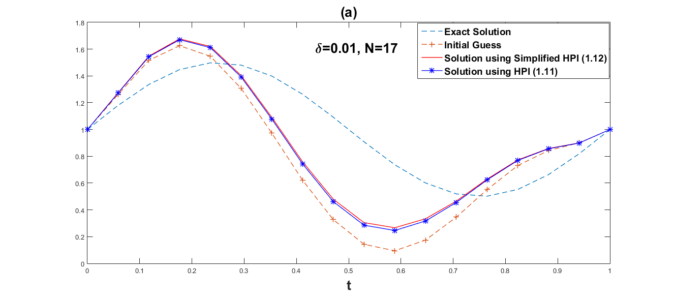
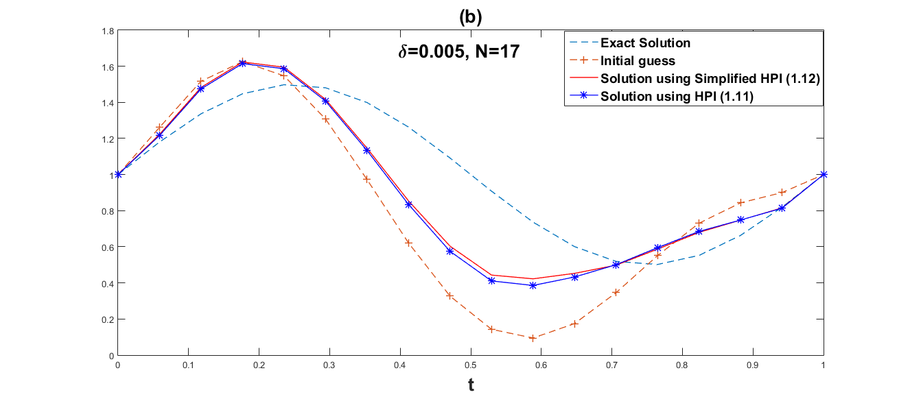
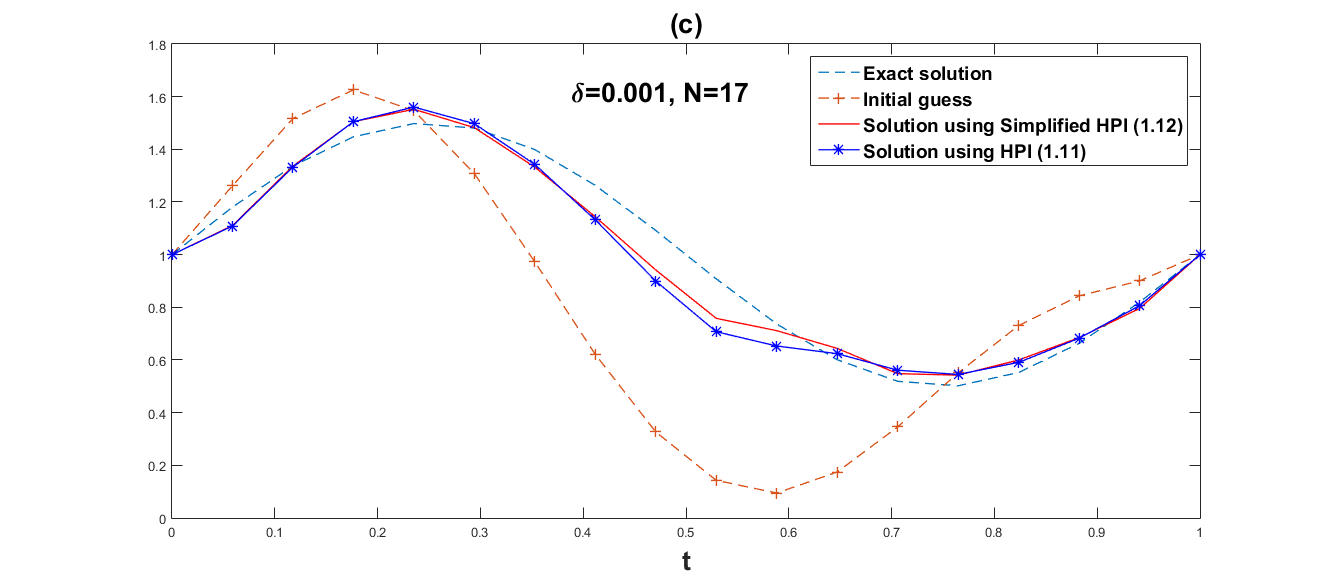
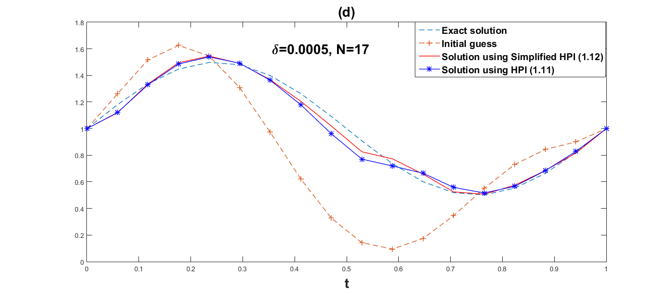
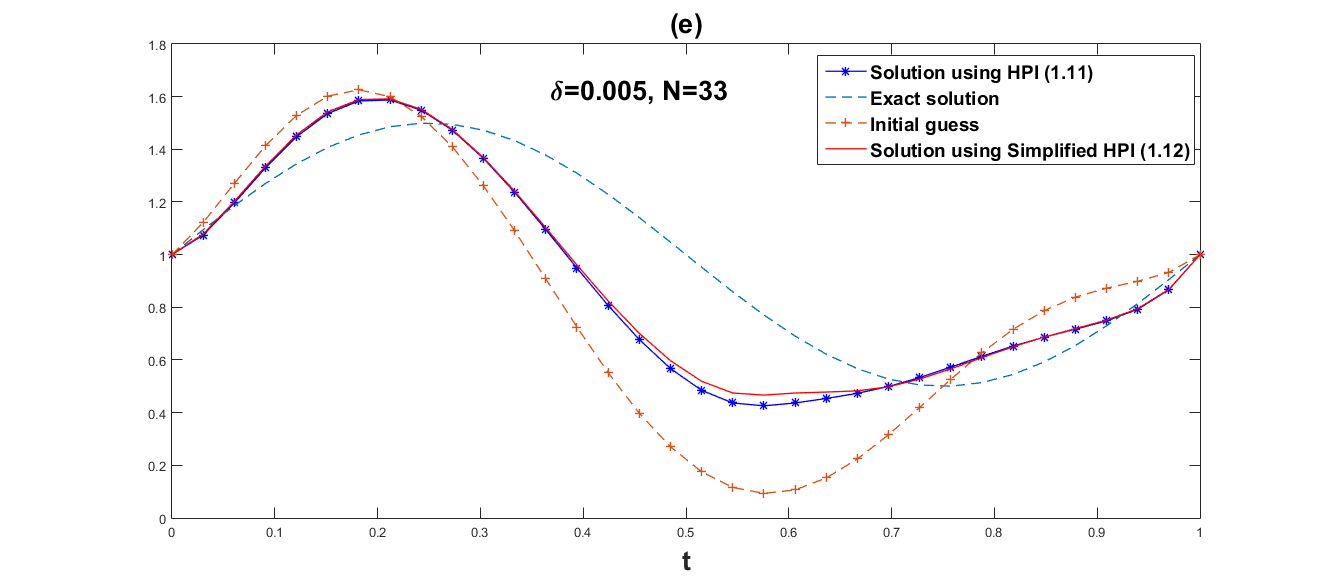
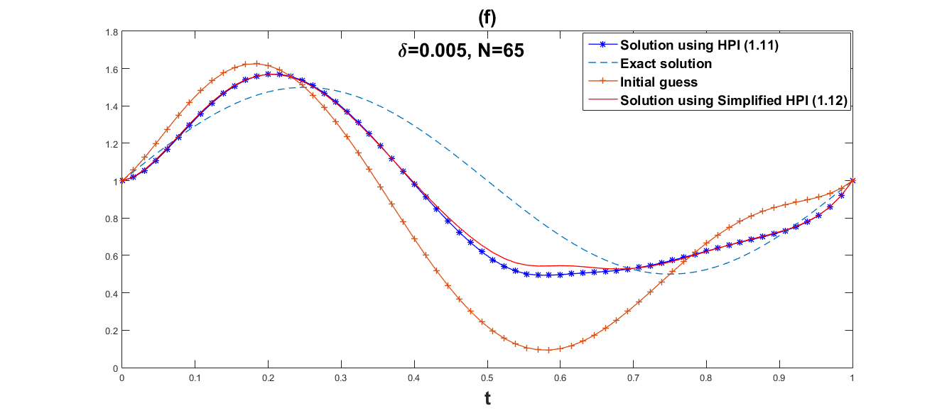
Assume that $\mathrm{\Omega }=[0,1]$. The right-hand side of differential equation (47) is explicitly determined using exact information $u^{†}(t)$. By introducing random noise to the precise data $u^{†}(t)$ at a specified noise level $\delta$, the perturbed data $u^{\delta }(t)$ satisfying $\Vert u^{\delta }(t)-u^{†}(t)\Vert \le \delta$ is obtained. On a uniform grid with different grid points (N), the differential equations involving the Fréchet differentiable (48) are solved using the finite element method using linear splines. With $\tau =5$, the iteration is terminated using the stopping criteria (17).

We use the function

$$f(t)=-e^t(1+\frac{1}{2}\sin (2\pi t)+\pi \cos (2\pi t))+(e-1)\pi \cos (2\pi t),$$

and the exact data $u^{†}(t)=e^t+(1-e)t-1$, so the exact solution is $c^{†}(t)=1+\frac{1}{2}\sin (2\pi t)$.

We start the iteration with the initial guess

$$c_0(t)=1+\frac{1}{2}sin(2\pi t)+200t^2{(1-t)}^2(0.25-t)(0.75-t).$$

Then, according to [22]: $c_0-c^{†}=200t^2{(1-t)}^2(0.25-t)(0.75-t)\in R(F^{\prime }{(x^{†})}^{\ast })$.

We employ both the suggested simplified Homotopy perturbation iteration (12) and the Homotopy perturbation iteration (11). Several values of $\delta$ and grid point $N$ are chosen in order to show how the convergence rates depend on the noise level. The numerical results are given in Table 1 and Table 2. Fig. 1–Fig. 6 respectively, represent graphical results for the methods (11) and (12).

Obviously, Fig. 1–Fig. 6 show that the approximate effect of simplified Homotopy perturbation iteration is better. Compared with Homotopy perturbation iteration, we discover in Table 1 and Table 2 that the error norm of simplified Homotopy perturbation iteration is much smaller within less iteration steps and less computational time, and also the convergent rate of simplified Homotopy perturbation iteration (12) is faster than Homotopy perturbation iteration (11).

$\delta$	N	$n_{\delta }$	$Error=\Vert c_{n_{\delta }}^{\delta }-c^{†}\Vert$	Time(s)
0.01	17	424	1.3377	1.5375
0.005	17	4853	0.9980	16.9290
0.001	17	53252	0.2844	189.9022
0.0005	17	134204	0.1877	421.6156
0.01	33	1972	1.6762	8.7951
0.005	33	8511	1.1900	31.0274
0.01	65	4457	2.0520	21.7195
0.005	65	13948	1.3607	75.8592

Table 1. The results of the Simplified HPI (12).

$\delta$	N	$n_{\delta }$	$Error=\Vert c_{n_{\delta }}^{\delta }-c^{†}\Vert$	Time(s)
0.01	17	510	1.3569	1.8747
0.005	17	5970	1.0488	18.4612
0.001	17	83441	0.3475	265.8005
0.0005	17	189874	0.2529	628.5853
0.01	33	2350	1.7366	9.1521
0.005	33	10628	1.2667	42.0180
0.01	65	5312	2.1569	26.6291
0.005	65	18020	1.4721	91.1350

Table 2. The results of the HPI (11).

Figure 1. Solution when $N=17$ and $\delta =0.01$

Figure 2. Solution when $N=17$ and $\delta =0.005$

Figure 3. Solution when $N=17$ and $\delta =0.001$

Figure 4. Solution when $N=17$ and $\delta =0.0005$

Figure 5. Solution when $N=33$ and $\delta =0.005$

Figure 6. Solution when $N=65$ and $\delta =0.005$

5. Conclusion

In this study, we have performed the analysis and evaluated a simplified version of the Homotopy perturbation iteration (11). The suggested technique has the advantage of just computing the Fréchet derivative once, rather than at each iteration step. The calculation in this approach becomes simpler than the traditional Homotopy perturbation iterations, as the iteration (12) and the source condition (25) only entail the Fréchet derivative at initial guess $x_0$ to the exact solution $x^{†}$ of (1). The suggested iteration is competitive in terms of reducing the overall computing time as well as error when compared to the traditional Homotopy perturbation iteration as demonstrated by the numerical example.

References

- [1]
- [2] A. B. Bakushinskii, The problem of the iteratively regularized Gauss–Newton method, Comput. Math. Math. Phys., 32 (1992), pp. 1353–1359.
- [3] A. B. Bakushinskii, Iterative methods for solving non-linear operator equations without condition of regularity, Soviet. Math. Dokl., 330 (1993), pp. 282–284.
-
[4]
A. Binder, M. Hanke and O. Scherzer, On the Landweber iteration for nonlinear ill-posed problems, J. Inverse Ill-Posed Probl., 4 (1996), no. 5, pp. 381–389.
https://doi.org/10.1515/jiip.1996.4.5.381
![[Uncaptioned image]](ext-link.png)
- [5] H. W. Engl, M. Hanke and A. Neubauer, Regularization of Inverse problems, Math. Appl., 375, Kluwer Academic publishers group, Dordrecht, 1996.
- [6] H. W. Engl, K. Kunisch and A. Neubauer, Convergence rates for Tikhonov regularization of nonlinear ill-posed problems, Inverse Problems, 5 (1989), no. 4, pp. 523–540.
- [7] H. S. Fu, L. Cao, B. Han, A homotopy perturbation method for well log constrained seismic waveform inversion. Chin. J. Geophys.-Chinese Edition, 55 (2012), no. 9, pp. 3173–3179.
[8]
M. Hanke, A. Neubauer and O. Scherzer, A convergence analysis of the Landweber iteration for nonlinear ill-posed problems, Numer. Math., 72 (1995), no. 1, pp. 21–37.
https://doi.org/10.1007/s002110050158
- [9] Q. Jin Q, A general convergence analysis of some Newton-Type methods for nonlinear inverse problems. SIAM J. Numer. Anal., 49 (2011), no. 49, pp. 549–573.
[10]
Q. Jin, On a regularized Levenberg–Marquardt method for solving nonlinear inverse problems, Numer. Math., 115 (2010), no. 2, pp. 229–259.
https://doi.org/10.1007/s00211-009-0275-x
[11]
J. Jose and M. P. Rajan, A Simplified Landweber Iteration for Solving Nonlinear Ill-Posed Problems, Int. J. Appl. Comput. Math., 3 (2017), no. 1, pp. 1001–1018.
https://doi.org/10.1007/s40819-017-0395-4
- [12] B. Kaltenbacher, A. Neubauer and O. Scherzer, Iterative Regularization Methods for Nonlinear Ill-Posed Problems, De Gruyter, New York (2008).
[13]
B. Kaltenbacher,Regularization by projection with a posteriori discretization level choice for linear and nonlinear ill-posed problems, Inverse Problems, 16 (2000), pp. 1523–1539.
https://doi.org/10.1088/0266-5611/16/5/322
- [14] L. Cao, B. Han, W. Wang, Homotopy perturbation method for nonlinear ill-posed operator equations, J. Nonlinear Sci. Numer. Simul., 10 (2009), no. 10, pp. 1319–1322.
[15]
L. Cao, B. Han, Convergence analysis of the Homotopy perturbation method for solving nonlinear ill-posed operator equations, Comput. Math. Appl., 61 (2011), no. 8, pp. 2058–2061.
https://doi.org/10.1016/j.camwa.2010.08.069
[16]
P. Mahale, M. Nair, A simplified generalized Gauss-Newton method for nonlinear ill-posed problems, Math. Comp., 78 (2009), no. 265, pp. 171–184.
https://doi.org/10.1090/S0025-5718-08-02149-2
[17]
P. Mahale, Simplified iterated Lavrentiev regularization for nonlinear ill-posed monotone operator equations, Comput. Methods Appl. Math., 17 (2017), no. 2, pp. 269–285.
https://doi.org/10.1515/cmam-2016-0044
- [18] P. Mahale and P. K. Dadsena, Simplified Generalized Gauss–Newton Method for Nonlinear Ill-Posed Operator Equations in Hilbert Scales, Comput. Methods Appl. Math., 18 (2018), no. 4, pp. 687–702.
- [19] P. Mahale and K. D. Sharad, Error estimate for simplified iteratively regularized Gauss-Newton method in Banach spaces under Morozove Type stopping rule, J. Inverse Ill-Posed Probl., 20 (2017), no. 2, pp. 321–341.
[20]
P. Mahale and K. D. Sharad, Convergence analysis of simplified iteratively regularized Gauss-Newton method in Banach spaces setting, Appl. Anal., 97 (2018), no. 15, pp. 2686–2719.
https://doi.org/10.1080/00036811.2017.1386785
[21]
A. Neubauer, On Landweber iteration for nonlinear ill-posed problems in Hilbert scales, Numer. Math., 85 (2000), pp. 309–328.
https://doi.org/10.1007/s002110050487
[22]
O. Scherzer,
A modified Landweber iteration for solving parameter estimation problems, Appl. Math. Optim., 38 (1998), pp. 45–68.
https://doi.org/10.1007/s002459900081
[23]
Convergence criteria of iterative methods based on Landweber iteration for solving nonlinear problems. J. Math. Anal. Appl., 194 (1995), pp. 911–933.
https://doi.org/10.1006/jmaa.1995.1335
[24]
O. Scherzer, H. W. Engl and K. Kunisch, Optimal a posteriori parameter choice for Tikhonov regularization for solving nonlinear ill-posed problems, SIAM J. Numer. Anal., 30 (1993), pp. 1796–1838.
https://doi.org/10.1137/0730091