Return to Article Details Dynamics of a model of nonlocal dispersion viral infection that includes humoral immunity, intracellular delay, and virus-to-cell and cell-to-cell transmissions

Dynamics of a model of nonlocal dispersion viral infection that includes humoral immunity, intracellular delay, and virus-to-cell and cell-to-cell transmissionsThanks: Corresponding author email: djilali.salih@yahoo.fr, s.djilali@univ-chlef.dz
¹Laboratory of Mathematics Modeling and Applications, University of Adrar
National Road No. 06, 01000, Adrar, Algeria.
²Department of Mathematics, Faculty of Exact Sciences and informatics,
Hassiba Benbouali University, Chlef, Algeria

Boubakr Lamouri¹, Ahmed Boudaoui¹ and Salih Djilali²

Date: November 11, 2025; accepted: June 30, 2026; published online: August 31, 2026.

Abstract.

This paper investigates a delayed spatiotemporal viral infection model with two types of transmissions, namely, virus-to-cell transmission, and cell-to-cell transmission, and a special focus on the cell-mediated immunity. First, we establish that the model system has a global attractor and that the model admits a unique positive solution which is globally defined. The basic reproduction numbers of immunity $\Re_{1}$ and infection $\Re_{0}$ are then determined. The immunity-related reproduction number $\Re_{1}$ is defined only when $\Re_{0}>1$ , which serves as a threshold parameter. Indeed, it is obtained that the infection-free steady state is globally asymptotically stable when $\Re_{0}<1$ , the immunity-free infected steady state is globally asymptotically stable when $\Re_{1}\leq 1<\Re_{0}$ , and the infected-immune steady state is globally asymptotically stable when $\Re_{1}>1$ . Finally, numerical simulation is performed in order to validate our theoretical results.

Key words and phrases:

Global attractor, cell-to-cell transmission, nonlocal diffusion, basic reproduction number, uniform persistence.

2005 Mathematics Subject Classification

92B, 35B, 58Z

1. Introduction

Viral dynamics is a well-established branch of applied mathematics that aims to describe the temporal evolution of infected cells and viral load through mathematical modeling. During viral infection, the specific immune response plays a crucial role in controlling disease progression. This response includes both cell-mediated immunity, driven by cytotoxic T lymphocytes (CTLs), and humoral immunity, mediated by antibodies produced by B cells. Since the pioneering work of Nowak and Bangham [1], a wide range of mathematical models have been developed to investigate immune responses against infected cells [9]–[15].

To better understand the interplay between virus dynamics and immune response, we focus on a transmission mechanism that incorporates both virus-to-cell and cell-to-cell infection pathways. In this context, Jiazhe and Rui [2] proposed the following basic viral dynamic model:

(1)	$\displaystyle S^{\prime}(\iota)$	$\displaystyle=\lambda-\beta S(\iota)I(\iota)-\alpha S(\iota)V(\iota)-\beta_{S}S(\iota),$
	$\displaystyle V^{\prime}(\iota)$	$\displaystyle=\beta e^{-\mu\tau_{V}}S(\iota-\tau_{V})I(\iota-\tau_{V})+\alpha e^{-\mu\tau_{V}}S(\iota-\tau_{V})V(\iota-\tau_{V})-\beta_{V}V(\iota),$
	$\displaystyle I^{\prime}(\iota)$	$\displaystyle=\beta_{1}V(\iota)-\gamma_{1}I(\iota)R(\iota)-\beta_{I}I(\iota),$
	$\displaystyle R^{\prime}(\iota)$	$\displaystyle=\zeta I(\iota)R(\iota)-\beta_{R}R(\iota).$

Here, $S$ , $I$ , $V$ , and $R$ represent the densities of uninfected cells, infected cells, free virus particles, and B cells, respectively. The parameters describe biological processes such as infection rates, natural death rates, immune response activation, and viral production. The delay $\tau_{V}$ accounts for the intracellular period between viral entry and the release of new virions, while $e^{-\mu\tau_{V}}$ represents the survival probability during this latent phase.

It is well known that viruses can spread over relatively long distances within biological tissues, for instance through blood circulation or intercellular transport mechanisms. Therefore, the classical diffusion operator, typically modeled by the Laplacian, may not adequately capture such long-range movements, as it only describes local interactions based on infinitesimal displacements. In contrast, nonlocal diffusion operators provide a more realistic framework by incorporating spatial interactions over a finite range.

Specifically, nonlocal diffusion is often modeled by an integral operator of the form

\int_{\Omega}J(\eta-\vartheta)\big(\Psi(\iota,\vartheta)-\Psi(\iota,\eta)\big)\,d\vartheta,

where $J(\cdot)$ is a dispersal kernel describing the probability of movement from location $\vartheta$ to $\eta$ . Unlike classical diffusion, this operator accounts for long-range dispersal and allows individuals (or particles) to move directly between distant locations. From a biological perspective, this is particularly relevant for viral propagation, where transport mechanisms are not purely local.

Another important distinction concerns boundary conditions. In classical diffusion models, no-flux (Neumann) boundary conditions are imposed through local derivatives. However, in the nonlocal framework, the dispersal process inherently involves interactions across the entire domain $\Omega$ . As a result, boundary effects are implicitly incorporated into the integral operator, provided that the kernel $J$ is properly defined (for instance, with compact support or normalization conditions). In this work, we complement the nonlocal formulation with homogeneous Neumann-type conditions to ensure consistency with biological assumptions of no net outward flux.

Moreover, to enhance biological realism, we incorporate time delays representing the latent period between infection and viral production, as well as the activation delay of the immune response. Such delays have been widely studied in the literature [17, 22, 24], mainly in the context of virus-to-cell transmission. However, their combined effect with cell-to-cell transmission and nonlocal dispersal remains less understood.

Motivated by the above considerations, we propose the following delayed viral dynamic model with nonlocal diffusion:

(2)		$\displaystyle\tfrac{\partial S}{\partial\iota}=$	$\displaystyle\lambda_{1}(\eta)-\beta_{S}(\eta)S-\beta(\eta)SI-\alpha(\eta)SV,$
	$\displaystyle\tfrac{\partial V}{\partial\iota}=$	$\displaystyle\beta(\eta)S(\iota-\tau_{v},\eta)I(\iota-\tau_{v},\eta)e^{-\mu\tau_{V}}$
		$\displaystyle+\alpha(\eta)S(\iota-\tau_{v},\eta)V(\iota-\tau_{v},\eta)e^{-\mu\tau_{V}}-\beta_{V}(\eta)V,$
	$\displaystyle\tfrac{\partial I}{\partial\iota}=$	$\displaystyle K_{I}\int_{\Omega}J(\eta-\epsilon)(I(\iota,\epsilon)-I(\iota,\eta))\,d\epsilon+\beta_{1}(\eta)V-\beta_{I}(\eta)I-\gamma_{1}(\eta)IR,$
	$\displaystyle\tfrac{\partial R}{\partial\iota}=$	$\displaystyle K_{R}\int_{\Omega}J(\eta-\epsilon)(R(\iota,\epsilon)-R(\iota,\eta))\,d\epsilon$
		$\displaystyle+\zeta(\eta)I(\iota-\tau_{R},\eta)R(\iota-\tau_{R},\eta)-\beta_{R}(\eta)R.$

with $\iota>0$ and $\eta\in\Omega$ . The associated initial and boundary conditions are given by

(3)		$\displaystyle S(l,\eta)=$	$\displaystyle S_{0}(l,\eta),\!I(l,\eta)=I_{0}(l,\eta),\!\!V(l,\eta)=V_{0}(l,\eta),R(l,\eta)=R_{0}(l,\eta),$
		$\displaystyle(l,\eta)\in[-\tau,0]\times\bar{\Omega}$

and

\tfrac{\partial I}{\partial n}=\tfrac{\partial R}{\partial n}=0,\quad\eta\in\partial\Omega,\ \iota>0,

where $K_{R}$ and $K_{I}$ are the diffusion coefficients. $\tau_{R}$ is the period of time needed for antigenic stimulation generating antibody response, $\bar{\Omega}\subset\mathbb{R}^{n}$ is a bounded set with smooth boundary (represents the position).

Let $\tau=\max\{\tau_{v},\tau_{R}\}$ . Every parameter should be positive, space-dependent, and Hölder continuous on $\bar{\Omega}$ .

The paper is structured as follows. We will examine the well-posedness of (2) and (3) in Section 2. In Section 3, we utilize Kuratowski’s measure of non-compactness to demonstrate the existence of a global compact attractor for the semiflow. The purpose of Section 4 is to determine the basic reproduction numbers of immunity $\Re_{1}$ and infection $\Re_{0}$ . Keep in mind that for $\Re_{1}$ to be defined, $\Re_{0}$ must be greater than 1. Section 5: A triple dynamics is the primary outcome. In Section 6, when $\Re_{1}\leq 1<\Re_{0}$ , the immunity-free infected steady state is globally asymptotically stable, when $\Re_{1}>1$ , the infected-immune steady state is globally asymptotically stable. These are the general terms used to describe the infection-free steady state and immunity-free infected steady state. Section 7 is configured to demonstrate the use of numerical simulation.

2. Preliminaries

We make the following assumptions on the system parameters (2)–(3):

(P0)

$\mathbf{J}(\eta)$ is Lipschitz continuous on $\overline{\Omega}$ .
(P1)

$\mathbf{J}$ is symmetric, non-negative and normalized: $\mathbf{J}(-z)=\mathbf{J}(z)$ on $\mathbb{R}^{n}$ , $\int_{\Omega}\mathbf{J}(z)\,dz=1$ , and $\mathbf{J}(z)>0$ on $\overline{\Omega}$ .

Let $\mathbb{X}=C([-\tau,0]\times\overline{\Omega},\mathbb{R}),\quad X=\mathbb{X}^{4},$ equipped with the supremum norm $\|\cdot\|_{\infty}$ . Denote by $\mathbb{X}_{+}$ and $X_{+}$ the associated positive cones. Throughout this work, all model parameters are assumed to be nonnegative, bounded, and continuous on $\overline{\Omega}$ . For notational convenience, given any function $\mathcal{H}\in C(\overline{\Omega},\mathbb{R})$ , we define $\mathcal{H}^{+}:=\sup_{\eta\in\overline{\Omega}}\mathcal{H}(\eta),\quad\mathcal{H}^{-}:=\inf_{\eta\in\overline{\Omega}}\mathcal{H}(\eta)$ , with $\mathcal{H}\in\{\lambda_{1},\beta,\alpha,\mu,\beta_{V_{1}},\beta_{V_{2}},\beta_{V_{3}},\beta_{V_{4}}\}.$

We now provide a few standard results taking into account the model’s well-posedness (2)–(3). Model (2)–(3) can be rewritten in the following abstract form

(4)

\tfrac{d\mathbb{U}}{d\iota}(\iota)=\mathit{A[\mathbb{U}](\iota)+F[\mathbb{U}](\iota)}\text{ ,}\mathbb{U}(\iota)\in X_{+},

with

AU=\left(\begin{array}[]{r}A_{1}\mathbb{U}_{1}\\ A_{2}\mathbb{U}_{2}\\ A_{3}\mathbb{U}_{3}\\ A_{4}\mathbb{U}_{4}\end{array}\right)=\left(\begin{array}[]{c}-\beta_{S}(v)S(\iota,\cdot)\\ -\beta_{V}(\eta)V(\iota,\cdot)\\ K_{I}\int_{\Omega}J(\eta-y)(I(\iota,y)-I(\iota,\eta))dy-\beta_{I}(\eta)I(\iota,\cdot)\\ K_{R}\int_{\Omega}J(\eta-y)(R(\iota,y)-R(\iota,\eta))dy-\beta_{R}(\eta)R(\iota,\cdot)\end{array}\right),

and

\mathit{F\mathbb{U}}=\left(\begin{array}[]{c}\lambda_{1}(\eta)-\beta(\eta)S(\iota,\cdot)I(\iota,\cdot)-\alpha(\eta)S(\iota,\cdot)V(\iota,\cdot)\\ \beta S(\iota-\tau_{v},.)I(\iota-\tau_{v},\cdot)e^{-\mu\tau_{V}}+\alpha S(\iota-\tau_{v},\cdot)V(\iota-\tau_{v},\cdot)e^{-\mu\tau_{V}}\\ \beta_{1}(\eta)V(\iota,\cdot)-\gamma_{1}(\eta)I(\iota,\eta)R(\iota,\cdot)\\ \zeta(\eta)I(\iota-\tau_{R},\cdot)R(\iota-\tau_{R},\cdot)\end{array}\right).

The following linear operator should be defined on $C(\bar{\Omega})$ .

A_{I}[\Phi](\cdot):=K_{I}\int_{\Omega}J(\eta-y)(\Phi(y)-\Phi(\cdot))dy-\beta_{I}(\cdot)\Phi(\cdot)\text{; }\Phi\in C(\bar{\Omega}).

Some properties on $A$ are given by the following lemma.

Lemma .

$A$ generates a strictly contractive and uniformly continuous semigroup $\{e^{A\iota}\}_{\iota\geq 0}$ .
Additionally, $e^{A\iota}X_{+}\subset X_{+}$ $\forall$ $\iota\geq 0$ .

Proof.

It is possible to break down operator $A$ as $A=A_{1}+A_{2}$ , with

A_{1}\mathbb{U}=\left(\begin{array}[]{c}-\beta_{S}S(\iota,\cdot)\\ -\beta_{V}V(\iota,\cdot)\text{ }\\ -\beta_{I}I(\iota,\cdot)\\ -\beta_{R}R(\iota,\cdot)\end{array}\right),A_{2}\mathbb{U}=\left(\begin{array}[]{c}0\\ 0\text{ }\\ K_{I}\int_{\Omega}J(\eta-\epsilon)(I(\iota,\epsilon)-I(\iota,\cdot))d\epsilon\\ K_{R}\int_{\Omega}J(\eta-\epsilon)(R(\iota,\epsilon)-R(\iota,\cdot))d\epsilon\end{array}\right),

for $\mathbb{U}\in X$ . Therefore, a uniformly continuous and strictly contractive semigroup $\{e^{A\iota}\}_{\iota_{\geq 0}}$ on $X$ is generated by $A_{1}$ . We may deduce that $A_{2}$ is a Lipschitz function since $J$ is bounded. $A$ generates a $C_{0}$ -semigroup $\{e^{A\iota}\}_{\iota\geq 0}$ , by Theorem 1.2 in [4] and Corollary VI.1.11 in [5].

∎

Theorem 1.

Suppose that $\mathbb{U}_{0}=(\varphi_{1}(b,\eta),\varphi_{2}(b,\eta),\varphi_{3}(b,\eta))\in X$ . Hence, there exists $\tau_{{}_{0}}>0$ such that (2)-(3) has unique positive solution $\mathbb{U}(\cdot,\mathbb{U}_{0})\in X$ , such that either $\tau_{{}_{0}}=\infty$ or $\underset{{}_{\iota\rightarrow\tau_{0^{-}}}}{\lim}\sup\|\mathbb{U}(\iota,\mathbb{U}_{0})\|=\infty$ .
Moreover, $\mathbb{U}(\iota,\mathbb{U}_{0})\in X_{+}$ for $\iota\in(0,\tau_{0})$ if $\mathbb{U}_{0}\in X_{+}$ .

Proof.

The solution of system (2)-(3) can be written as follows

(5)

\mathbb{U}(\iota)=\mathbb{U}_{0}e^{A\iota}+\int_{0}^{\iota}e^{A(\iota-s)}F(\mathbb{U}(s))ds.

The function $\mathit{F}:X\rightarrow X$ is locally Lipschitz on $X$ . As established by Lemma 3.1 in [6], Proposition 4.16 in [7] guarantees that system (2) has a unique mild solution, denoted by $\mathbb{U}(.,\mathbb{U}_{0})$ , where $\tau_{0}$ verifies either $\tau_{0}=\infty$ or $\displaystyle\limsup_{\iota\to\tau_{0}^{-}}\|\mathbb{U}(\iota,\mathbb{U}_{0})\|=\infty$ .

Now, we show $S(\iota,\eta)>0$ for $\iota\in(0,\tau_{0})$ and $\eta\in\bar{\Omega}$ . We suppose that $\exists$ $\overset{\sim}{\tau}\in(0,\tau_{0})$ and $\eta_{{}_{0}}\in\Omega$ verifying that $S(\overset{\sim}{\tau},\eta_{{}_{0}})=0$ and $S(\iota,\eta_{{}_{0}})>0$ for $\iota<\overset{\sim}{\tau}$ . Next, we can specify

\tau_{1}=\inf\Big\{\iota\in(0,\tau_{0});S(\iota,\eta_{{}_{0}})=0\Big\}.

Since $\tau_{0}$ satisfies $\tau_{0}=\infty$ or $\displaystyle\limsup_{\iota\to\tau_{0}^{-}}\|\mathbb{U}(\iota,\mathbb{U}_{0})\|=\infty.$ , then we deduce that $\tau_{1}\in(0,\tau_{0})$ and $S(\overset{\sim}{\tau},\eta_{{}_{0}})=0$ with $\tfrac{\partial S(\overset{\sim}{\tau},\eta)}{\partial\iota}\leq 0$ . The first equation of (2) yields

\tfrac{\partial S(\tau_{1},\eta_{{}_{0}})}{\partial\iota}=\lambda_{1}(\eta_{{}_{0}})>0,

that contradicts the assumptions. Hence, $S(\iota,\eta)>0$ for $\iota\in(0,\tau_{0})$ , $\eta\in\bar{\Omega}$ .

We put $A_{h_{r}}(\mathbb{U})=\mathbb{U}(\iota,\cdot)+h_{r}\mathbb{U}(\iota,\cdot)$ for a sufficiently large positive $h_{r}$ . For $\mathbb{U}\in C((0,\tau_{0}),X)\cap$ ß $(0,\tfrac{1}{h_{r}})$ , obviously $A_{h_{r}}(\mathbb{U})$ is positive. In conjunction with the open ball ß $(0,\tfrac{1}{h_{r}})$ in $X$ , with radius $\tfrac{1}{h_{r}}$ and center $0$ . Hence, (2) can be reworded as this:

\tfrac{d\mathbb{U}}{d\iota}(\tau)=A_{h_{r}}[\mathbb{U}](\iota)+F_{h_{r}}[\mathbb{U}](\iota).\text{ }

with $A_{h_{r}}\mathbb{U}(\iota,\cdot)=\mathbb{U}(\iota,\cdot)-h_{r}\mathbb{U}(\iota,\cdot)$ . Then,

U(\iota)=U_{0}(\eta)e^{A_{h_{r}}\iota}+\int_{0}^{\iota}e^{A_{h_{r}}(\iota-s)}F_{h_{r}}(U(s))ds.\text{ \ \ }

Hence, $\mathbb{U}(\iota,\mathbb{U}_{0})\in X_{+}$ for $\iota\in(0,\tau_{0})$ and $\mathbb{U}_{0}\in X_{+}$ . ∎

Theorem 2.

The solution of (2)–(3) is globally defined.

Proof.

Let $\mathbb{U}=(S,I,V,R)$ be the solution associated to $\mathbb{U}_{0}=(S_{0},I_{0},V_{0},R_{0})$ . Since $\ \tfrac{dS}{dt}(\iota,\eta)\leq\lambda(\eta)-\beta_{S}S(\iota,\eta)$ , $\check{S}$ is a subsolution of

(6)

\left\{\begin{array}[]{lll}\tfrac{\partial\check{S}}{\partial\iota}(\iota,\eta)=\lambda_{1}(\eta)-\beta_{S}\check{S}(\iota,\eta),\quad\eta\in\Omega,\quad\iota>0,&&\\[5.69054pt] \check{S}(0,\eta)=\underset{s\in[-\tau,0]}{\max}S_{0}(s,\eta),\quad\eta\in\Omega.&&\end{array}\right.

The unique positive steady state of (6), represented by $\check{S}_{f}$ , is globally attractive and well known. By the comparison theorem, we get

\displaystyle\limsup_{\iota\rightarrow\infty}S(\iota,\eta)\leq\displaystyle\limsup_{\iota\rightarrow\infty}\check{S}(\iota,\eta)=\check{S}_{f}(\eta)=\tfrac{\lambda_{1}(\eta)}{\beta_{s}(\eta)}\text{ uniformly for }\eta\in\Omega.

Consequently, $\exists K>0$ that depends on $\mathbb{U}_{0}$ such that

\|S\|\leq K\text{,}\ \iota>0.

Next, we let $A_{I}$ be the generator of the uniformly continuous semigroup $\{T_{1}(\iota)\}_{\iota_{\geq 0}}$

	$\displaystyle I(\iota,\cdot)$	$\displaystyle=T_{1}(\iota)I_{0}+\int\limits_{0}^{\iota}T_{1}(\iota-\sigma)(\beta_{1}V(\sigma,\cdot)-\gamma_{1}(x)I(\sigma,\cdot)R(\sigma,\cdot))d\sigma,$
		$\displaystyle\leq T_{1}(\iota)I_{0}+\int\limits_{0}^{\iota}T_{1}(\iota-\sigma)\beta_{1}V(\sigma,\cdot)d\sigma.$

By taking the norm on both sides, we obtain

\|I(\iota,\cdot)\|\leq e^{-\lambda\iota}\|I_{0}\|+\|\beta_{1}\|\int\limits_{0}^{\iota}e^{-\lambda(\iota-\sigma)}\|V(\sigma,\cdot)\|d\sigma.

We assume that the eigenvalue for the operator $A_{I}$ is $-\lambda$ . According to Proposition 1 in [8], $\exists c>0$ fulfills $\lambda>c>0$ . The second equation of (2)–(3) suggests

V(\iota,\cdot)=e^{-\beta_{V}\iota}V_{0}+\int\limits_{0}^{\iota}e^{-\beta_{V}(\iota-\sigma)}(e^{-\mu\tau_{V}}S(\sigma-\tau_{v},\cdot)(\beta I(\sigma-\tau_{v},\cdot)+\alpha V(\sigma-\tau_{v},\cdot))d\sigma.

Therefore,

		$\displaystyle\\|V(\iota;.)\\|\leq$
		$\displaystyle\leq e^{-\beta_{V}\iota}\\|V_{0}\\|$
		$\displaystyle\quad+\int\limits_{0}^{\iota}e^{-\beta_{V}(\iota-\sigma)}e^{-\mu\tau_{V}}\\|S(\sigma-\tau_{v},\cdot)\\|(\\|\beta\\|\\|I(\sigma-\tau_{v},\cdot)\\|+\\|\alpha\\|\\|V(\sigma-\tau_{v},\cdot)\\|)d\sigma,$
		$\displaystyle\leq e^{-\beta_{V}\iota}\\|V_{0}\\|+Ke^{-\mu\tau_{V}}\int\limits_{0}^{\iota}e^{-\beta_{V}(\iota-\sigma)}(\\|\beta\\|\\|I(\sigma-\tau_{v},\cdot)\\|+\\|\alpha\\|\\|V(\sigma-\tau_{v},\cdot)\\|)d\sigma,$
		$\displaystyle\leq e^{-\beta_{V}\iota}\\|V_{0}\\|+K\beta^{\ast}e^{-\mu\tau_{V}}\int\limits_{0}^{\iota}e^{-\beta_{V}(\iota-\sigma)}(\\|I(\sigma-\tau_{v},\cdot)\\|+\\|V(\sigma-\tau_{v},\cdot)\\|)d\sigma,$

where $\beta^{\ast}=\max\{\|\beta\|,\|\alpha\|\}$ . Using the substitution $\sigma^{\ast}=\sigma-\tau_{v}$ and dropping tilde for simplicity, thus,

		$\displaystyle\\|V(\iota,\cdot)\\|\leq$
		$\displaystyle\leq e^{-\beta_{V}\iota}\\|V_{0}\\|+K\beta^{\ast}e^{-\mu\tau_{V}}\int\limits_{\tau_{v}}^{\iota-\tau_{v}}e^{-\beta_{V}(\iota-\tau_{v}-\sigma)}(\\|I(\sigma,\cdot)\\|+\\|V(\sigma,\cdot)\\|)d\sigma$
		$\displaystyle\leq e^{-\beta_{V}\iota}\\|V_{0}\\|+K\beta^{\ast}e^{-\mu\tau_{V}}\int\limits_{\tau_{v}}^{\iota-\tau_{v}}e^{-\beta_{V}(\iota-\tau_{v}-\sigma)}\\|V(\sigma,\cdot)\\|d\sigma$
		$\displaystyle\quad+K\beta^{\ast}e^{-\mu\tau_{V}}\int\limits_{\tau_{v}}^{\iota-\tau_{v}}e^{-\beta_{V}(\iota-\tau_{v}-\sigma)}\\|I(\sigma,\cdot)\\|d\sigma.$

Thus,

		$\displaystyle\\|V(\iota,\cdot)\\|\leq$
		$\displaystyle\leq e^{-\beta_{V}\iota}\\|V_{0}\\|+K\beta^{\ast}e^{-\mu\tau_{V}}\int\limits_{\tau_{v}}^{\iota-\tau_{v}}e^{-\beta_{V}(\iota-\tau_{v}-\sigma)}\\|V(\sigma,\cdot)\\|d\sigma$
		$\displaystyle\quad+K\beta^{\ast}e^{-\mu\tau_{V}}\int\limits_{\tau_{v}}^{\iota-\tau_{v}}e^{-\beta_{V}(\iota-\tau_{v}-\sigma)}\left\{e^{-\lambda\sigma}\\|I_{0}\\|+\\|\beta_{1}\\|_{0}^{\sigma}e^{-\lambda(\sigma-s)}\\|V(s,\cdot)\\|ds\right\}d\sigma$
		$\displaystyle\leq e^{-\beta_{V}\iota}\\|V_{0}\\|+K\beta^{\ast}e^{-\mu\tau_{V}}\int\limits_{\iota_{v}}^{\iota-\tau_{v}}e^{-\beta_{V}(\tau-\tau_{v}-\sigma)}\\|V(\sigma,\cdot)\\|d\sigma$
		$\displaystyle\quad+K\beta^{\ast}e^{-\mu\tau_{V}}\\|I_{0}\\|\int\limits_{-\tau_{v}}^{\iota-\tau_{v}}e^{-\beta_{V}(\iota-\tau_{v}-\sigma)}e^{-\lambda\sigma}d\sigma$
		$\displaystyle\quad+\\|\beta_{1}\\|K\beta^{\ast}e^{-\mu\tau_{V}}\int\limits_{-\tau_{v}}^{\iota-\tau_{v}}e^{-\beta_{V}(\iota-\tau_{v}-\sigma)}\int\limits_{-\tau_{v}}^{\sigma}e^{-\lambda(\sigma-s)}\\|V(s,\cdot)\\|dsd\sigma$
		$\displaystyle\leq e^{-\beta_{V}\iota}\\|V_{0}\\|+K\beta^{\ast}e^{-\mu\tau_{V}}\int\limits_{-\tau_{v}}^{\iota-\tau_{v}}e^{-\beta_{V}(\tau-\tau_{v}-\sigma)}\\|V(\sigma,\cdot)\\|d\sigma$
		$\displaystyle\quad+K\beta^{\ast}e^{-\mu\tau_{V}}\\|I_{0}\\|\int\limits_{-\tau_{v}}^{\iota-\tau_{v}}e^{-\lambda\sigma}d\sigma$
		$\displaystyle\quad+\\|\beta_{1}\\|M\beta^{\ast}e^{-\mu\tau_{V}}\int\limits_{-\tau_{v}}^{\iota-\tau_{v}}e^{-\beta_{V}(\iota-\tau_{v}-\sigma)}\int\limits_{-\tau_{v}}^{\sigma}e^{-\lambda(\sigma-s)}\\|V(s,.)\\|dsd\sigma.\text{ }$

Consequently,

		$\displaystyle\\|V(\iota,\cdot)\\|\leq$
		$\displaystyle\leq e^{-\beta_{V}\iota}\\|V_{0}\\|+K\beta^{\ast}e^{-\mu\tau_{V}}\int\limits_{-\tau_{v}}^{\iota-\tau_{v}}e^{-\beta_{V}(\tau-\tau_{v}-\sigma)}\\|V(\sigma,\cdot)\\|d\sigma$
		$\displaystyle\quad+K\beta^{\ast}e^{-\mu\tau_{V}}\\|I_{0}\\|\tfrac{e^{\lambda\tau_{v}}-e^{-\lambda(\iota-\tau_{v})}}{\lambda}$
		$\displaystyle\quad+\\|\beta_{1}\\|K\beta^{\ast}e^{-\mu\tau_{V}}e^{-\beta_{V}(\iota-\tau_{v})}\int\limits_{-\tau_{v}}^{\iota-\tau_{v}}e^{\lambda s}\\|V(s,\cdot)\\|\int\limits_{s}^{\iota-\tau_{v}}e^{(\beta_{V}-\lambda)\sigma}d\sigma ds$
		$\displaystyle\leq e^{-\beta_{V}\tau}\\|V_{0}\\|+K\beta^{\ast}e^{-\mu\tau_{V}}\int\limits_{-\tau_{v}}^{\iota-\tau_{v}}e^{-\beta_{V}(\tau-\tau_{v}-\sigma)}\\|V(\sigma,\cdot)\\|d\sigma$
		$\displaystyle\quad+K\beta^{\ast}e^{-\mu\tau_{V}}\\|I_{0}\\|\tfrac{e^{\lambda\tau_{v}}-e^{-\lambda(\iota-\tau_{v})}}{\lambda}$
		$\displaystyle\quad+\\|\beta_{1}\\|K\beta^{\ast}e^{-\mu\tau_{V}}\tfrac{e^{-\varpi(\tau-\tau_{v})}}{\lambda-\beta_{V}}\int\limits_{-\tau_{v}}^{\iota-\tau_{v}}e^{\varpi s}\\|V(s,\cdot)\\|ds$
		$\displaystyle\leq\\|V_{0}\\|+K\beta^{\ast}e^{-\mu\tau_{V}}\int\limits_{-\tau_{v}}^{\iota-\tau_{v}}e^{-\varpi(\tau-\tau_{v}-\sigma)}\\|V(\sigma,\cdot)\\|d\sigma$
		$\displaystyle\quad+K\beta^{\ast}e^{-\mu\tau_{V}}\\|I_{0}\\|\tfrac{e^{\lambda\tau_{v}}}{\lambda}$
		$\displaystyle\quad+\tfrac{\\|\beta_{1}\\|K\beta^{\ast}e^{-\mu\tau_{V}}}{\lambda-\beta_{V}}\int\limits_{-\tau_{v}}^{\iota-\tau_{v}}e^{-\varpi(\iota-\tau_{v}-s)}\\|V(s,\cdot)\\|ds$
		$\displaystyle\leq C_{1}+C_{2}\int\limits_{-\tau_{v}}^{\iota-\tau_{v}}\\|V(s,\cdot)\\|ds,$

with

	$\displaystyle\varpi$	$\displaystyle=\min\left\{\beta_{V}^{-},\tfrac{\lambda}{2}\right\},C_{1}=\\|V_{0}\\|+K\beta^{*}e^{-\mu\tau_{V}}\\|I_{0}\\|\tfrac{e^{\lambda\tau_{V}}}{\lambda},$
	$\displaystyle C_{2}$	$\displaystyle=\max\left\{K\beta^{}e^{-\mu\tau_{V}},\tfrac{\\|\beta_{1}\\|K\beta^{}e^{-\mu\tau_{V}}}{\lambda-\beta_{V}}\right\}.$

Gronwall’s inequality implies

\displaystyle\|V\|

\displaystyle\leq C_{1}e^{C_{2}\iota}\text{, }\iota\geq 0.

The last equation of (2) implies

\displaystyle R(\iota,.)=e^{-\beta_{R}\iota}R_{0}+\int\limits_{0}^{\iota}\zeta(x)e^{-\beta_{R}(\iota-\sigma)}I(\sigma-\tau_{R},x)R(\iota-\tau_{R},x)d\sigma.

Therefore, $\sigma^{\ast\ast}=\sigma-\tau_{R}$

\|R(\iota,.)\|\leq e^{-\beta_{R}\iota}\|R_{0}\|+\zeta^{\ast}\int\limits_{-\tau_{R}}^{\iota-\tau_{R}}e^{-\beta_{R}(\iota-\sigma)}\|I(\sigma,\cdot)\|\|R(\sigma,\cdot)\|d\sigma.

It follows

(7)

\displaystyle\|R(\iota,\cdot)\|

\displaystyle\leq C_{4}e^{C_{5}\iota}\text{, }\iota\geq 0,

with

	$\displaystyle\\|I(\iota,\cdot)\\|$	$\displaystyle\leq\\|I_{0}\\|+\tfrac{C_{1}\\|\beta_{1}\\|e^{C_{2}\iota}}{\lambda}=C_{3},$
	$\displaystyle\\|I(\iota,\cdot)\\|$	$\displaystyle\leq\\|I_{0}\\|e^{-\lambda\iota}+\\|\beta_{1}\\|\int_{0}^{\iota}e^{-\lambda(\iota-\sigma)}\\|V(\sigma,\cdot)\\|d\sigma$
		$\displaystyle\leq\\|I_{0}\\|e^{-\lambda\iota}+C_{1}\\|\beta_{1}\\|\int_{0}^{\iota}e^{-\lambda(\iota-\sigma)}e^{C_{2}\iota}d\sigma$
		$\displaystyle\leq\\|I_{0}\\|+\tfrac{C_{1}\\|\beta_{1}\\|e^{C_{2}\iota}}{\lambda}=C_{3}.$

Therefore, the solution is globally defined, that is, $\tau_{0}=+\infty$ . ∎

3. Compactness

We now examine the solution map’s compactness. The semiflow produced by system (2)–(3) is denoted by $\{\Xi(\iota)\}_{\iota\geq 0}$ . $\Xi(\iota)$ is not compact. we may demonstrate the asymptotic compactness of forward orbits in order to demonstrate that $\Xi(\iota)$ has a global compact attractor. Thus, using Kuratowski measure $\kappa$ , which is defined as follows,

\kappa(\mathbf{B})=\inf\left\{r\text{: has a finite cover of diameter}<r\right\}.

Then

\mathbf{B}\text{ precompact}\Leftrightarrow\kappa(P)=0.

To achieve this goal, we apply several lemmas.

Lemma .

The semiflow $\{\Xi(\iota)\}_{\iota_{\geq 0}}$ is point dissipative.

Proof.

We let $H(\iota,\eta)=S(\iota,\eta)+V(\iota+\tau_{v},\eta)$ ; hence,

	$\displaystyle\tfrac{\partial H(\iota,\eta)}{\partial\iota}$	$\displaystyle=\lambda_{1}(\eta)-(1-e^{-\mu\tau_{V}})\beta(\eta)S(\iota,\eta)I(\iota,\eta)$
		$\displaystyle\quad-(1-e^{-\mu\tau_{V}})\alpha(\eta)S(\iota,\eta)V(\iota,\eta)-\beta_{S}(\eta)S(\iota,\eta)-\beta_{V}(\eta)V(\iota+\tau_{v},\eta)$
		$\displaystyle\leq\text{ }\lambda_{1}(\eta)-\beta_{S}(\eta)S(\iota,\eta)-\beta_{V}(\eta)V(\iota+\tau_{v},\eta)$
		$\displaystyle\leq\text{ }\lambda_{1}(\eta)-\omega H(\iota,\eta)$

with $\omega=\min\{\beta_{S}^{-},\beta_{V}^{-}\}$ . Therefore, we get $H(\iota,\eta)\leq g_{1}(\eta)$ , $\iota\in\mathbb{R}^{+}$ , with $g_{1}(\eta)=H(0,\eta)+\tfrac{\lambda_{1}(\eta)}{\omega}$ . Therefore, the existence of $\xi_{1}$ independent of the initial conditions verifying

\underset{\iota\rightarrow\infty}{\lim}\sup\|H(\iota,\eta)\|\leq\xi_{1}.

On $\Omega$ ,we integrate the third equation of (2).

	$\displaystyle\tfrac{\partial}{\partial\iota}\int_{\Omega}I(\iota,\eta)d\eta=$	$\displaystyle K_{I}\int_{\Omega}\int_{\Omega}J(\eta-\epsilon)(I(\iota,\epsilon)-I(\iota,\eta))d\epsilon d\eta$
		$\displaystyle+\int_{\Omega}\beta_{1}(\eta)V(\iota,\eta)d\eta-\int_{\Omega}\beta_{I}(\eta)I(\iota,\eta)d\eta$
		$\displaystyle-\int_{\Omega}\gamma_{1}(\eta)I(\iota,\eta)R(\iota,\eta)d\eta,$
	$\displaystyle\leq$	$\displaystyle\int_{\Omega}\beta_{1}(\eta)V(\iota,\eta)d\eta-\mathbf{\beta}_{I}^{-}\int_{\Omega}I(\iota,\eta)d\eta,$

which gives

\tfrac{\partial}{\partial\iota}\int_{\Omega}I(\iota,\eta)d\eta+\mathbf{\beta}_{I}^{-}\int_{\Omega}I(\iota,\eta)d\eta\leq\int_{\Omega}\beta_{1}(\eta)V(\iota,\eta)d\eta.

Let us multiply by $e^{\mathbf{\beta}_{I}^{-}\iota}$ ,

	$\displaystyle e^{\mathbf{\beta}_{I}^{-}\iota}\tfrac{\partial}{\partial\iota}\int_{\Omega}I(\iota,\eta)d\eta+\mathbf{\beta}_{I}^{-}e^{\mathbf{\beta}_{I}^{-}\iota}\int_{\Omega}I(\iota,\eta)d\eta$	$\displaystyle\leq$	$\displaystyle e^{\mathbf{\beta}_{I}^{-}\iota}\int_{\Omega}\beta_{1}(\eta)V(\iota,\eta)d\eta,$
	$\displaystyle\tfrac{d}{d\iota}e^{\mathbf{\beta}_{I}^{-}\iota}\int_{\Omega}I(\iota,\eta)d\eta$	$\displaystyle\leq$	$\displaystyle e^{\mathbf{\beta}_{I}^{-}\iota}\int_{\Omega}\beta_{1}(\eta)V(\iota,\eta)d\eta,$

Integrating by parts, we find

	$\displaystyle\int_{0}^{\iota}\tfrac{\partial}{\partial s}e^{\mathbf{\beta}_{I}^{-}s}\int_{\Omega}I(s,\eta)d\eta ds$	$\displaystyle\leq\int_{0}^{\iota}e^{\mathbf{\beta}_{I}^{-}s}\int_{\Omega}\beta_{1}(\eta)V(s,\eta)d\eta ds,$
	$\displaystyle e^{\mathbf{\beta}_{I}^{-}\iota}\int_{\Omega}I(\iota,\eta)d\eta+\int_{\Omega}I(0,\eta)d\eta$	$\displaystyle\leq\int_{0}^{\iota}e^{\mathbf{\beta}_{I}^{-}s}\int_{\Omega}\beta_{1}(\eta)V(s,\eta)d\eta ds,$
	$\displaystyle\int_{\Omega}I(\iota,\eta)d\eta$	$\displaystyle\leq e^{-\mathbf{\beta}_{I}^{-}\iota}\int_{\Omega}I(0,\eta)d\eta$
		$\displaystyle\quad+\tfrac{1}{\mathbf{\beta}_{I}^{-}}(1-e^{-\mathbf{\beta}_{I}^{-}\iota})\int_{\Omega}\beta_{1}(\eta)V(s,\eta)d\eta:=D_{1}.$

On the other hand, we have

	$\displaystyle\tfrac{\partial}{\partial\iota}I(\iota,\eta)d\eta$	$\displaystyle=$	$\displaystyle K_{I}\int_{\Omega}J(\eta-\epsilon)(I(\iota,\epsilon)-I(\iota,\eta))d\epsilon+\beta_{1}(\eta)V(\iota,\eta)-\beta_{I}(\eta)I(\iota,\eta)$
		$\displaystyle\leq$	$\displaystyle K_{I}(\underset{\eta\in\Omega}{\sup}J)\int_{\Omega}I(\iota,\epsilon)d\epsilon+\beta_{1}(\eta)V(\iota,\eta)-\beta_{I}(\eta)I(\iota,\eta).$

By applying this inequality, the third equation in (2) suggests

\tfrac{dI(\iota,\cdot)}{d\iota}\leq K_{I}(\underset{\eta\in\Omega}{\sup}J)D_{1}+\beta_{1}^{+}\xi_{1}-(K_{I}+\beta_{I}^{-})I(\iota,\cdot).

Then,

I(\iota,\cdot)\leq I_{0}(\iota,\cdot)e^{-(K_{I}+\beta_{I}^{-})\iota}+\tfrac{K_{I}(\underset{\eta\in\Omega}{\sup}J)D_{1}+\beta_{1}^{+}\xi_{1}}{K_{I}+\beta_{I}^{-}}(1-e^{-(K_{I}+\beta_{I}^{-})\iota}).

After that, $\exists\xi_{2}$ independent of the initial condition satisfying

\displaystyle\limsup_{\iota\rightarrow\infty}\|I(\iota,\eta)\|\leq\xi_{2}.

We integrate the final equation of (2) on $\Omega$

	$\displaystyle\tfrac{\partial}{\partial\iota}\int_{\Omega}R(\iota,\eta)dx=$	$\displaystyle K_{R}\int_{\Omega}\int_{\Omega}J(\eta-\epsilon)(R(\iota,\epsilon)-R(\iota,\eta))d\epsilon d\eta$
		$\displaystyle+\int_{\Omega}\zeta(\eta)V(\iota-\tau_{R},\eta)I(\iota-\tau_{R},\eta)d\eta-\int_{\Omega}\beta_{R}(\eta)R(\iota,\eta)d\eta$
	$\displaystyle\leq$	$\displaystyle\text{ }\int_{\Omega}\zeta(\eta)R(\iota-\tau_{R},\eta)I(\iota-\tau_{R},\eta)d\eta-\beta_{R}^{-}\int_{\Omega}R(\iota,\eta)d\eta.$

By similar reasoning, there is a $\xi_{3}$ independent of the initial condition satisfying

\displaystyle\limsup_{\iota\rightarrow\infty}\|R(\iota,\eta)\|\leq\xi_{3}.

Therefore, the semiflow $\Xi(\iota)$ is point dissipative. ∎

We now demonstrate that $\Xi(\iota)$ is a $\kappa$ $-$ contraction; that is, for all $\iota>0$ , there exists a continuous function $0\leq k(\iota)<1$ , and a bounded set $\theta$ , such that $\{\Xi(\sigma)\theta,0\leq\sigma\leq\iota\}$ is bounded and $\kappa(\Xi(\sigma)\theta)\leq k(\iota)\kappa(\theta)$ . First, we demonstrate the asymptotic compactness of $S$ and $V$ .

Lemma .

The forward orbit $\ \delta^{+}(\Psi):\mathbb{U}(\iota,\cdot,\mathbb{U}_{0}),\iota\geq 0$ for (2)–(3) is asymptotically compact for all $\Psi\in X^{+}$ , in that for all sequences $\iota_{k}\rightarrow\infty$ . Consequently, $\exists\iota_{ki}$ to satisfy $\mathbb{U}(\iota_{ki},\cdot;\mathbb{U}_{0})$ converges in $X^{+}$ as $i$ $\rightarrow\infty$ .

Proof.

Let us assume that $\mathbb{U}_{0}\in X^{+}$ , there exists $\eta>0$ verifying

\mid S(\iota,\eta;\mathbb{U}_{0})\mid\leq\varpi,\ \mid I(\iota,\eta;\mathbb{U}_{0})\mid\leq\varpi,\ for\text{ }all\text{ }\eta\in\overset{-}{\Omega},\ \iota\geq 0.

It is sufficient to demonstrate that $\mathbb{U}(\iota,\eta;\mathbb{U}_{0})_{n\geq 1}$ is equicontinuous in $\eta\in\bar{\Omega},$ $\iota>0$ using the Arzelà–Ascoli theorem. In other words, for all $\rho>0$ , there exists $\varepsilon>0$ guaranteeing $|h(\iota,\eta_{1})-h(\iota,\eta_{2})|<\varepsilon^{2}$ for all $\ \eta_{1},\eta_{2}\in\bar{\Omega}$ as long as $|\eta_{1}-\eta_{2}|<\rho$ . It is evident that $h(\iota,\eta)=\lambda(\eta)+\beta(\eta)S(\iota,\eta)I(\iota,\eta)e^{-\mu\tau_{V}}+\alpha(\eta)S(\iota,\eta)V(\iota,\eta)e^{-\mu\tau_{V}}$ is uniformly continuous in $\eta\in\bar{\Omega}$ uniformly for $\iota\geq 0$ . Clearly,

		$\displaystyle\!\!\!\!\!\!\tfrac{\partial}{\partial\iota}\left[S(\iota,\eta_{1})-S(\iota,\eta_{2})\right]^{2}=$
	$\displaystyle=$	$\displaystyle 2(S(\iota,\eta_{1})-S(\iota,\eta_{2}))\Big[h(\iota,\eta_{1})-h(\iota,\eta_{2})-\beta_{S}(\eta_{1})(S(\iota,\eta_{1})\Big.$
		$\displaystyle\left.-S(\iota,\eta_{2}))-S(\iota,\eta_{2})(\beta_{S}(\eta_{1})-\beta_{S}(\eta_{2}))\right]$
	$\displaystyle\leq$	$\displaystyle 4\eta(h(\iota,\eta_{1})-h(\iota,\eta_{2}))-\beta_{S}(\eta_{1})(S(\iota,\eta_{1})-S(\iota,\eta_{2})){2}$
		$\displaystyle+\mid S(\iota,\eta_{2})\cdot(\beta_{S}(\eta_{1})-\beta_{S}(\eta_{2}))\mid$
	$\displaystyle\leq$	$\displaystyle(4\varpi\varepsilon^{2}+2\varepsilon)-\beta_{S}^{-}(\eta_{1})(S(\iota,\eta_{1})-S(\iota,\eta_{2}))^{2},$

for all $\iota>$ $-\tau_{V}$ and $\eta_{1},\eta_{2}\in\bar{\Omega}$ verifying $|\eta_{1}-\eta_{2}|<\rho$ , we have

\left[S(\iota,\eta_{1})-S(\iota,\eta_{2})\right]^{2}\leq e^{-\beta_{S}^{-}\iota}\left[\left[S(0,\eta_{1})-S(0,\eta_{2})\right]^{2}\right]+(4\varpi\varepsilon^{2}+2\varepsilon)\int_{0}^{\iota}e^{-2\beta_{S}^{-}(\iota-\sigma)}d\sigma.

Then

\left[S(\iota,\eta_{1})-S(\iota,\eta_{2})\right]^{2}\leq\left[S(0,\eta_{1})-S(0,\eta_{2})\right]^{2}+(4\varpi\varepsilon^{2}+2\varepsilon)\int_{0}^{\iota}e^{-2\beta_{S}^{-}(\iota-\sigma)}d\sigma.

Given that $\eta\in\bar{\Omega}$ , the initial condition’s uniform continuity suggests that $\mid S_{0}(0,\eta_{1})-S_{0}(0,\eta_{2})\mid<\tfrac{\varepsilon}{2}$ for all $\eta_{1},\eta_{2}\in\bar{\Omega}$ verifying that $|\eta_{1}-\eta_{2}|<\rho_{1}$ . Therefore, for any $|\eta_{1}-\eta_{2}|<$ $min\{\rho,\rho_{1}\}$ , with $\eta_{1},\eta_{2}\in\overset{-}{\Omega}$ , we have

\left[S(\iota,\eta_{1})-S(\iota,\eta_{2})\right]^{2}\leq\tfrac{\varepsilon^{2}}{4}+\tfrac{(4\varpi\varepsilon^{2}+2\varepsilon)}{2\beta_{S}^{-}}.

Since $S$ is equicontinuous, we can infer that $\varepsilon$ is arbitrary. We demonstrate that $I$ , $V$ and $R$ are equicontinuous by using a similar logic. ∎

Lemma .

The semiflow $\Xi(\iota)$ is a $\kappa$ -contraction.

Proof.

Clearly, $I(\iota,\eta,\mathbb{U}_{0})$ and $R(\iota,\eta,\mathbb{U}_{0})$ satisfy

	$\displaystyle\tfrac{\partial I}{\partial\iota}(\iota,\eta)$	$\displaystyle=K_{I}\int_{\Omega}J(\eta-\epsilon)(I(\iota,\epsilon)-I(\iota,\eta))d\epsilon-\beta_{I}(\eta)I(\iota,\eta),$
	$\displaystyle\tfrac{\partial R}{\partial\iota}(\iota,\eta)$	$\displaystyle=K_{R}\int_{\Omega}J(\eta-\epsilon)(R(\iota,\epsilon)-R(\iota,\eta))d\epsilon-\beta_{R}(\eta)R(\iota,\eta),$
	$\displaystyle I(s,\eta)$	$\displaystyle=I_{0}(s,\eta),R(s,\eta)=R_{0}(s,\eta),\text{ }s\in[-\tau,0],\text{ }\eta\in\overset{-}{\Omega}.$

Therefore,

I(\iota,\cdot)=T_{1}(\iota)I_{0}+\int\limits_{0}^{\iota}T_{1}(\iota-\sigma)(\beta_{1}(\cdot)V(\sigma,\cdot,\mathbb{U}_{0})-\gamma_{1}(\cdot)I(\sigma,\cdot,\mathbb{U}_{0})R(\sigma,\cdot,\mathbb{U}_{0}))d\sigma,

and

R(\iota,\cdot)=T_{2}(\iota)R_{0}+\zeta(\cdot)\int\limits_{0}^{\iota}T_{2}(v-\sigma)V(\sigma-\tau_{R},\cdot,\mathbb{U}_{0})I(\sigma-\tau_{R},\cdot,\mathbb{U}_{0})d\sigma,

according to Lemma 2.1 in [10], the operators $L_{V}$ and $L_{R}$ have strictly positive eigenfunctions, which correspond to strictly negative eigenvalues $\mu_{0}$ and $\mu_{1}$ , respectively. These eigenvalues are defined by

\mu_{0}=-\inf_{\begin{subarray}{c}\Psi_{0}\in L^{2}(\Omega)\\ \|\Psi_{0}\|_{L^{2}(\Omega)}=1\end{subarray}}\Bigg\{\!\!\int_{\Omega}\int_{\Omega}J(\eta-\varepsilon)\bigl(\Psi_{0}(\varepsilon)-\Psi_{0}(\eta)\bigr)^{2}\,d\varepsilon\,d\eta\!+\!\!\int_{\Omega}\beta_{I}(\eta)\Psi_{0}^{2}(\eta)\,d\eta\Bigg\},

and

\mu_{1}=-\inf_{\begin{subarray}{c}\Psi_{1}\in L^{2}(\Omega)\\ \|\Psi_{1}\|_{L^{2}(\Omega)}=1\end{subarray}}\!\!\Bigg\{\int_{\Omega}\int_{\Omega}J(\eta-\varepsilon)\bigl(\Psi_{1}(\varepsilon)-\Psi_{1}(\eta)\bigr)^{2}\,d\varepsilon\,d\eta\!+\!\!\int_{\Omega}\beta_{R}(\eta)\Psi_{1}^{2}(\eta)\,d\eta\Bigg\}.

Now, we decompose the semiflow into $\Phi(\iota)=\Phi_{1}(\iota)+\Phi_{2}(\iota)$ , where

\Phi_{1}(\iota)U_{0}=(0,0,T_{1}(\iota)I_{0},T_{2}(\iota)R_{0}),\ \iota\geq 0

and

	$\displaystyle\Phi_{2}(\iota)\mathbb{U}_{0}=$	$\displaystyle\bigg(S(\cdot,\cdot,\mathbb{U}_{0}),V(\cdot,\cdot,\mathbb{U}_{0}),$
		$\displaystyle\quad\int_{0}^{\iota}T_{1}(\iota-\sigma)(\beta_{1}(\cdot)V(\sigma,\cdot,\mathbb{U}_{0})-\gamma_{1}(\cdot)I(\sigma,\cdot,\mathbb{U}_{0})R(\sigma,\cdot,\mathbb{U}_{0}))d\sigma,$
		$\displaystyle\quad\zeta(\cdot)\displaystyle\int_{0}^{\iota}T_{2}(\tau-\sigma)V(\sigma-\tau_{R},\cdot,\mathbb{U}_{0})I(\sigma-\tau_{R},\cdot,\mathbb{U}_{0})d\sigma\bigg),~~\iota\geq 0$

We infer that $S, V, I$ , and $R$ are asymptotically compact from Section 3. Consequently, $\Phi_{2}$ is compact. Thus, we have $\kappa(\Phi_{2}(\iota)\mathbf{A})=0$ for a bounded set $\mathbf{A}\subset X^{+}$ and $\iota\geq 0$ . Additionally,

$\displaystyle\\|\Phi_{1}(\iota)\mathbb{U}_{0}\\|$	$\displaystyle\leq$	$\displaystyle\\|e^{L_{V}\iota}\mathbb{U}_{0}+e^{L_{R}\iota}\mathbb{U}_{0}\\|$
	$\displaystyle\leq$	$\displaystyle e^{\mu_{0}\iota}\\|\mathbb{U}_{0}\\|+e^{\mu_{1}\iota}\\|\mathbb{U}_{0}\\|$
	$\displaystyle\leq$	$\displaystyle e^{\mu^{\ast}\iota}\\|\mathbb{U}_{0}\\|,\ \iota>0,$

with $\mu^{\ast}=\max\{\mu_{0},\mu_{1}\}$ Hence,

\|\Phi_{1}(\iota)\|\leq e^{\mu^{\ast}\iota}.

Hence, for $\iota>0$

\kappa(\Phi(\iota)\mathbf{A})\leq\kappa(\Phi_{1}(\iota)\mathbf{A})+\kappa(\Phi_{2}(\iota)\mathbf{A})\leq e^{\mu^{\ast}\iota}\kappa(\mathbf{A}).

The conclusion that follows is that $\Xi(\iota)$ is a $\kappa$ - contraction. ∎

We infer from Section 3 that the semiflow $\Xi(\iota)$ is point dissipative. Moreover, Section 3 shows that $\Xi(\iota)$ is a $\kappa$ -contraction. By Lemma 2.3.5 in [11], every $\kappa$ -contraction semiflow is asymptotically smooth. Furthermore, Theorem 2.6 in [12] implies that $\Xi(\iota)$ possesses a global compact attractor that attracts all bounded subsets of $X^{+}$ . We denote this attractor by $\mathbb{C}$ .

4. Basic reproduction number and steady-state

A steady-state $(S(\eta),V(\eta),I(\eta),R(\eta))$ of (2) is the solution of the following system

(8)		$\displaystyle 0=$	$\displaystyle\lambda_{1}(\eta)-\beta_{S}(\eta)S(\eta)-\beta(\eta)S(\eta)I(\eta)-\alpha(\eta)S(\eta)V(\eta),$
	$\displaystyle 0=$	$\displaystyle\beta(\eta)S(\eta)I(\eta)e^{-\mu\tau_{V}}+\alpha(\eta)S(\eta)V(\eta)e^{-\mu\tau_{V}}-\beta_{V}(\eta)V(\eta),$
	$\displaystyle 0=$	$\displaystyle K_{I}\int_{\Omega}J(\eta-\epsilon)(I(\epsilon)-I(\eta))d\epsilon+\beta_{1}(\eta)V(\eta)-\beta_{I}(\eta)I(\eta)-\gamma_{1}(\eta)I(\eta)R(\eta),$
	$\displaystyle 0=$	$\displaystyle K_{R}\int_{\Omega}J(\eta-\epsilon)(R(\epsilon)-R(\eta))d\epsilon+\zeta(\eta)I(\eta)R(\eta)-\beta_{R}(\eta)R(\eta),\quad\eta\in\overset{-}{\Omega}$

Clearly, (2) has a unique VFSS $H_{0}=(\tfrac{\lambda_{1}(\eta)}{\beta_{S}(\eta)},0,0,0),\eta\in\bar{\Omega}$ . We linearize (2) in order to get the basic reproduction number $\mathbf{\Re}_{0}$ corresponding to (2) at $H_{0}$ , we have

(9)		$\displaystyle\tfrac{\partial V}{\partial\iota}=$	$\displaystyle\beta(\eta)\tfrac{\lambda_{1}(\eta)}{\beta_{S}(\eta)}I(\iota-\tau_{v},\eta)e^{-\mu\tau_{V}}+\alpha(\eta)\tfrac{\lambda_{1}(\eta)}{\beta_{S}(\eta)}V(\iota-\tau_{v},\eta)e^{-\mu\tau_{V}}-\beta_{V}(\eta)V(\iota,\eta),$
	$\displaystyle\tfrac{\partial I}{\partial\iota}=$	$\displaystyle K_{I}\int_{\Omega}J(\eta-\epsilon)(I(\iota,\epsilon)-I(\iota,\eta))d\epsilon+\beta_{1}(\eta)V(\iota,\eta)$
		$\displaystyle-\beta_{I}(\eta)I(\iota,\eta)-\gamma_{1}(\eta)I(\iota,\eta)R(\iota,\eta),\quad\iota>0,\eta\in\overset{-}{\Omega}.$

We only take into consideration the subsystem because $S$ and $R$ are absent from the middle two equations

\left\{\begin{array}[]{c}\tfrac{\partial}{\partial\iota}\left(\begin{array}[]{c}V\\ I\end{array}\right)=\mathbf{A}\left(\begin{array}[]{c}V\\ I\end{array}\right),\text{ }\eta\in\Omega,\ \iota\geq 0,\\[5.69054pt] \tfrac{\partial I}{\partial\upsilon}=0,\text{ \ \ \ \ \ \ \ \ \ \ \ \ \ \ \ \ \ \ \ \ }\eta\in\partial\Omega,\text{\ }\iota\geq 0,\end{array}\right.

we define the following linear operators $\mathbf{\mathcal{B}},\mathbf{\mathcal{F}}:\mathbb{Z}\rightarrow\mathbb{Z}(\mathbb{Z}:=C(\Omega,\mathbb{R}^{2}))$ ,

(10)

\mathbf{\mathcal{B}}=\left(\begin{array}[]{cc}-\beta_{V}(\eta)&0\\ \beta_{1}(\eta)&A_{I}\end{array}\right),\text{ }\mathbf{\mathcal{F}=}\left(\begin{array}[]{cc}\beta(\eta)\tfrac{\lambda_{1}(\eta)}{\beta_{S}(\eta)}e^{-\mu\tau_{V}}&\alpha(\eta)\tfrac{\lambda_{1}(\eta)}{\beta_{S}(\eta)}e^{-\mu\tau_{V}}\\ 0&0\end{array}\right),

and the linear operator $\mathbf{A:=\mathcal{B}+\mathcal{F}}$

We designate $\mathbf{T}_{\mathbf{\mathcal{B}}}\mathbf{(\iota)}$ as the semigroup that $\mathbf{\mathcal{B}}$ generates. Therefore, we can define $\mathbf{\Re}_{0}$ as the spectral radius of $\mathbf{\mathcal{K}}$ , which is

\mathbf{\Re}_{0}=\mathfrak{r}(\mathbf{\mathcal{K}}).

Here, the next generation operator, $\mathbf{\mathcal{K:=-FB}}^{-1}$ , can be written as

\mathbf{\mathcal{K}}(\Theta)(\eta)=\mathbf{\mathcal{F}}(\eta)\int_{0}^{\infty}\mathbf{T}_{B}\mathbf{(\iota)}(\Theta)(\eta)d\iota,\Theta\in C(\overset{-}{\Omega},\mathbb{R}^{2}),\ \eta\in\overset{-}{\Omega.}

To derive a variational expression for the basic reproduction number $\Re_{0}$ , we obtain the following result.

Lemma .

$\Re_{0}=\mathfrak{r}(-\mathbf{\mathcal{FB}}^{-1})=r(d_{V}+d_{I})$ with $d_{V}=\beta\tfrac{\lambda_{1}}{\beta_{S}\beta_{V}}e^{-\mu\tau_{V}}$ and $d_{I}=-\alpha\beta_{1}e^{-\mu\tau_{V}}\tfrac{\lambda_{1}(x)}{\beta_{S}\beta_{V}}A_{I}^{-1}$ .

Proof.

Let $\phi=\mathbf{\mathcal{F}}\Psi$ and $\ \Psi=-\mathbf{\mathcal{B}}^{-1}\Theta$ . Clearly,

\left\{\begin{array}[]{c}\beta_{V}\Psi_{1}=\Theta_{1}\text{ \ \ \ \ \ \ \ \ }\\ \beta_{I}\Psi_{1}-A_{I}\Psi_{2}=\Theta_{2}.\end{array}\right.

Solving this system, we get

	$\displaystyle\Psi_{1}$	$\displaystyle=$	$\displaystyle\tfrac{\Theta_{1}}{\beta_{V}},\text{ \ \ }$
	$\displaystyle\Psi_{2}$	$\displaystyle=$	$\displaystyle A_{I}^{-1}(\beta_{I}\Psi_{1}-\Theta_{2}).$

Consequently,

	$\displaystyle\phi_{1}$	$\displaystyle=$	$\displaystyle d_{1}\Psi_{1}+d_{2}\Psi_{2},$
	$\displaystyle\phi_{2}$	$\displaystyle=$	$\displaystyle 0,\text{ }$

with $d_{1}=\beta\tfrac{\lambda_{1}}{\beta_{S}\beta_{V}}e^{-\mu\tau_{V}}+\alpha e^{-\mu\tau_{V}}\tfrac{\lambda_{1}\beta_{1}}{\beta_{S}\beta_{V}}A_{I}^{-1}$ , and $d_{2}=-A_{I}^{-1}\alpha\tfrac{\lambda_{1}}{\beta_{S}}e^{-\mu\tau_{V}}$ . Hence, we can write

-\mathbf{\mathcal{FB}}^{-1}\left(\begin{array}[]{c}\Theta_{1}\\ \Theta_{2}\end{array}\right)=\left(\begin{array}[]{c}d_{1}\Psi_{1}+d_{2}\Psi_{2}\\ 0\end{array}\right).

Iteratively, we get

(-\mathbf{\mathcal{FB}}^{-1})^{n}\left(\begin{array}[]{c}\Theta_{1}\\ \Theta_{2}\end{array}\right)=\left(\begin{array}[]{c}d_{1}^{n}\Psi_{1}+d_{1}^{n-1}d_{2}\Psi_{2}\\ 0\end{array}\right).

Hence $\|d_{I}^{n}\|\leq\|(-\mathbf{\mathcal{FB}}^{-1})^{n}\leq\|d_{1}^{n-1}\|(\|d_{1}\|+\|d_{2}\|)$ . By applying the squeeze theorem and Gelfand’s formula, we obtain $\mathit{r(-\mathbf{\mathcal{F}}}\mathbf{\mathcal{B}}^{-1}\mathit{)=\mathfrak{r}(d}_{1}\mathit{)}.$ Since $d_{1}=d_{V}+d_{I}$ , the proof is achieved. From Section 4, we get

(11)

\Re_{0}=\mathfrak{r}(d_{V}+d_{I}),

where $d_{V}=\tfrac{\beta\lambda_{1}}{\beta_{S}\beta_{V}}$ is the cell-to-cell transmission’s next generation operator, and $\ d_{I}=\tfrac{\alpha\lambda_{1}\beta_{1}}{\beta_{S}\beta_{V}}A_{I}^{-1}$ is the next generation operator for virus-to-cell transmission. The basic reproduction number for cell-to-cell transmission only, when virus-to-cell transmission is not present, is

(12)

\Re_{0}^{V}=\mathfrak{r}(d_{V})=\underset{\eta\in\overset{-}{\Omega}}{\max}\tfrac{\beta(\eta)\lambda_{1}(\eta)e^{-\mu\tau_{V}}}{\beta_{S}(\eta)\beta_{V}(\eta)}.

Furthermore, the basic reproduction number can also be stated by the following variational formula in the situation of virus-to-cell only:

(13)

\Re_{0}^{I}=\mathfrak{r}(d_{I})=\underset{\Theta\in L^{2},\Theta\neq 0}{\sup}\tfrac{\int_{\Omega}\tfrac{\alpha(\eta)\lambda_{1}(\eta)\beta(\eta)e^{-\mu\tau_{V}}}{\beta_{S}(\eta)\beta_{V}(\eta)}\Theta^{2}(\eta)d\eta}{K_{I}\int_{\Omega}\int_{\Omega}\tfrac{1}{2}J(\eta-\epsilon)(\Theta(\epsilon)-\Theta(\eta))^{2}d\epsilon d\eta+\int_{\Omega}\beta_{I}(\eta)\Theta^{2}(\eta)d\eta}.

Clearly, $\Re_{0}\leq$ $\Re_{0}^{V}$ $+\Re_{0}^{I}$ . The equality holds if $\tfrac{\beta(\eta)\lambda_{1}(\eta)}{\beta_{S}(\eta)\beta_{V}(\eta)}$ is space independent.
The basic reproduction number $\Re_{1}$ for the antibody response is determined by

\Re_{1}=\underset{\Theta\in L^{2},\Theta\neq 0}{\sup}\tfrac{\int_{\Omega}\zeta(\eta)I^{\ast\ast}(\eta)\Theta^{2}(\eta)d\eta}{K_{R}\int_{\Omega}\int_{\Omega}\tfrac{1}{2}J(\eta-\epsilon)(\Theta(\epsilon)-\Theta(\eta))^{2}d\epsilon d\eta+\int_{\Omega}\beta_{R}(\eta)\Theta^{2}(\eta)d\eta}.

∎

It is evident that $\Re_{1}$ is increasing in $\zeta(\eta)$ and $I^{\ast\ast}(\eta)$ , and decreasing in $\beta_{R}$ and $K_{R}$ . In particular, we obtain the spatially homogeneous model, where model (2)–(3) degenerates.

\Re_{1}=\tfrac{\zeta(\eta)I^{\ast\ast}(\eta)}{\beta_{R}(\eta)}.

Lemma .

$\Re_{0}-1$ and $\delta(\mathbf{A})$ have the same sign.

5. Extinction scenario of virus

Here, we show that for $\Re_{0}<1$ , the VFSS is globally stable. First, we use the following theorem to show that this steady state is locally stable:

Theorem 3.

$H_{0}$ is locally asymptotically stable if $\Re_{0}<1$ , and unstable if $\Re_{0}>1$ .

Proof.

To begin with, we notice that $\mathbf{A}_{\tau_{V}}$ , the generator of the linearized system (9), and $\mathbf{A}$ , the generator of the corresponding linear system without delay ( $\tau_{V}=0$ ), are not identical. Moreover, the principal eigenvalue of the problem is $S(\mathbf{A}_{\tau_{V}})$ .

(14)		$\displaystyle\beta(\eta)\tfrac{\lambda_{1}(\eta)}{\beta_{S}(\eta)}\Theta_{3}(\eta)e^{-\lambda\tau_{V}}e^{-\mu\tau_{V}}+\alpha(\eta)\tfrac{\lambda_{1}(\eta)}{\beta_{S}(\eta)}\Theta_{2}(\eta)e^{-\lambda\tau_{V}}e^{-\mu\tau_{V}}-\beta_{V}(\eta)\Theta_{2}(\eta)$
	$\displaystyle=\lambda\Theta_{2}(\eta),$
	$\displaystyle K_{I}\int_{\Omega}J(\eta-\epsilon)(\Theta_{3}(\iota,\epsilon)-\Theta_{3}(\iota,\eta))d\epsilon+\beta_{1}(\eta)\Theta_{2}(\eta)-\beta_{I}(\eta)\Theta_{3}(\eta)$
	$\displaystyle=\lambda\Theta_{3}(\eta),$

with $\mathbf{A}_{\tau_{V}}$ as the generator of the semigroup $P_{\tau_{V}}(\iota)$ related to the delayed linear system (9), for all $\ \eta\in\bar{\Omega}$ . The principal eigenvalue of the problem is $\delta(\mathbf{A})$ .

(15)		$\displaystyle\beta(\eta)\tfrac{\lambda_{1}(\eta)}{\beta_{S}(\eta)}\Theta_{3}(\eta)e^{-\mu\tau_{V}}+\alpha(\eta)\tfrac{\lambda_{1}(\eta)}{\beta_{S}(\eta)}\Theta_{2}(\eta)e^{-\mu\tau_{V}}-\beta_{V}(\eta)\phi_{2}(\eta)=$	$\displaystyle\lambda\Theta_{2}(\eta),$
	$\displaystyle K_{I}\int_{\Omega}J(\eta-\epsilon)(\Theta_{3}(\iota,\epsilon)-\Theta_{3}(\iota,\eta))d\epsilon+\beta_{1}(\eta)\Theta_{2}(\eta)-\beta_{I}(\eta)\Theta_{3}(\eta)=$	$\displaystyle\lambda\Theta_{3}(\eta).$

We determine that $\delta(A)$ has the same sign as $S(A_{\tau_{V}})$ by applying Theorem 9.2.1 in [14] to the eigenvalue problem associated with the first equation of (14) and (15). As a result, there is a sign difference between the exponential growth rate associated with the semi-group linked to the delayed system (14), known as $\omega(P_{\tau_{V}})$ ), and the one associated with $P(\iota)$ , the semi-group linked to the generator $\mathbf{A}$ . The exponential growth bound of $P(\iota)$ is now found and is defined as

\omega(\mathbb{T})=\max\left\{\delta(\mathbf{A}),\omega_{0}(\mathbb{T})\right\},

utilizing $e^{\omega_{0}(\mathbb{T})}:=\kappa(P(\iota))$ where $\ \kappa$ represents the non-compactness measure. Finding the sign of $\omega(P_{\tau_{V}})$ is necessary to demonstrate the local stability of $H_{0}$ . If $\omega(\mathbb{T})<0$ , then $H_{0}$ is locally asymptotically stable; if $\omega(\mathbb{T})>0$ , then $H_{0}$ is unstable. Since $\omega(\mathbb{T})$ and $\omega(P_{\tau_{V}})$ have the same sign, it is possible to infer the local asymptotic stability of VFSS by using Theorem 2.1 in [16] to determine the sign of $\omega(\mathbb{T})$ . Section 3 gives us $\omega_{0}\leq\mu_{0}<0$ . As a result, $H_{0}$ stability (or instability) is determined by $\delta(A)$ . Section 4 gives us that $\Re_{0}-1$ and $\delta(\mathbf{A})$ have the same sign. Consequently, if $R_{0}<1$ , then $H_{0}$ is locally asymptotically stable since $\delta(\mathbf{A})<0$ and $\omega(\mathbb{T})<0$ . Nevertheless, if $\Re_{1}\leq 1<\Re_{0}$ , $\delta(\mathbf{A})>0$ . Consequently, $\omega(\mathbb{T})=\delta(\mathbf{A})>0$ , and $H_{0}$ becomes unstable. ∎

The following lemma is used to construct test functionals.

Lemma .

Given the assumption that $\Re_{0}$ $<1$ , then there exists a $\rho>0$ that satisfies $\rho<1$ . It may be written as

(16)		$\displaystyle\mathcal{\rho}=\underset{\Theta\in L^{2},\Theta\neq 0}{\sup}\bigg\{$	$\displaystyle\tfrac{1}{K_{I}\int_{\Omega}\int_{\Omega}\tfrac{1}{2}J(\eta-\epsilon)(\Theta(\eta)-\Theta(\epsilon))\Theta(\eta)d\epsilon d\eta+\int_{\Omega}\beta_{I}(\eta)\Theta^{2}(\eta)d\eta}\times$
		$\displaystyle\times\int_{\Omega}\tfrac{\alpha(\eta)\lambda_{1}(\eta)\beta_{I}(\eta)e^{-\mu\tau_{V}}}{\beta_{S}(\eta)\beta_{V}(\eta)-\beta_{\ast}e^{-\mu\tau_{V}}\lambda(\eta)}\Theta^{2}(\eta)d\eta\bigg\}.$

Additionally, the following system is also satisfied by the positive functions $\Theta^{0}=(\Theta_{1}^{0}(\eta),\Theta_{2}^{0}(\eta))^{T}$ .

(17)		$\displaystyle 0=$	$\displaystyle-(\beta_{V}(\eta)-\alpha(\chi)\tfrac{\lambda_{1}(\eta)}{\beta_{S}(\eta)}e^{-\mu\tau_{V}})\Theta_{1}^{0}(\eta)+\beta_{1}(\eta)\Theta_{2}^{0}(\eta),\quad\eta\in\overset{-}{\Omega},$
	$\displaystyle 0=$	$\displaystyle\tfrac{1}{\rho}\beta(\eta)e^{-\mu\tau_{V}}\tfrac{\lambda_{1}(\eta)}{\beta_{S}(\eta)}\Theta_{1}^{0}(\eta)+K_{I}\int_{\Omega}J(-\epsilon)(\Theta_{2}^{0}(\iota,\epsilon)-\Theta_{2}^{0}(\iota,\eta))d\epsilon-\beta_{I}(\eta)\Theta_{2}^{0}(\eta),$
		$\displaystyle\eta\in\overset{-}{\Omega}.$

Proof.

Notice that for $\Re_{0}$ $<1$ , we obtain that $\Re(\eta):=\tfrac{\beta(\eta)\lambda_{1}(\eta)}{\beta_{S}(\eta)\beta_{V}(\eta)}$ $\leq 1$ . As a consequence, we use a different decomposition from ( $\mathbf{A}\mathit{:=}{\mathsf{B+F}}$ ) of the operator $\mathbf{A}$ as

(18)

\mathbf{A}:=\left(\begin{array}[]{cc}\beta_{V}(\eta)-\alpha(\eta)\tfrac{\lambda_{1}(\eta)}{\beta_{S}(\eta)}e^{-\mu\tau_{V}}&0\\ \beta_{1}(\eta)&A_{I}\end{array}\right)+\left(\begin{array}[]{cc}0&\beta(\eta)e^{-\mu\tau_{V}}\tfrac{\lambda_{1}(\eta)}{\beta_{S}(\eta)}\\ 0&0\end{array}\right):={\mathsf{B+F}}

We assume that the semigroup generated by $\ {\mathsf{B}}$ is $\mathbb{T}_{{\mathsf{B}}}(\iota)$ . Clearly, $S({\mathsf{B}})<0$ . We assume that $\rho$ is the spectral radius of $\mathbf{K}$ , which is

\rho=\mathfrak{r}(\mathbf{K})

Using $\mathbf{K}:=-\mathsf{F}\mathsf{B}^{-1}$ and applying Theorem 3.5 in [13], we conclude that if $\mathbf{\mathcal{R}}_{0}<1$ , then $\delta(\mathbf{A})<0$ and, consequently, $\rho<1$ . We then consider an eigenvalue $\varrho$ of $\mathbf{A}$ that solves the following problem

\varrho\Theta(\eta)=\mathit{A}[\Theta](\eta),\eta\in\overset{-}{\Omega,\Theta=(\Theta_{1}(\eta),\Theta_{2}(\eta))^{T}\in C(}\Omega,\mathbb{R}^{2}).

Next, we claim that the problem

(19)

{\mathsf{B}}\mathit{[}\Theta\mathit{](\eta)=\varrho{\mathsf{F}}[}\Theta\mathit{]}(\eta),\eta\in\overset{-}{\Omega},

has a unique principal eigenpair $(\eta^{\ast},\Theta^{0})$ that fulfills

\mathit{\rho=\mathfrak{r}(-}{\mathsf{FB}}^{-1}\mathit{)=\mathfrak{r}(-}{\mathsf{B}}^{-1}{\mathsf{F}}\mathit{)=}\tfrac{1}{\varrho^{\ast}}.

We assume that $\mathbb{T}_{{\mathsf{B}}}(\iota)$ is the semigroup related to the generator ${\mathsf{B}}$ in order to demonstrate this assertion. Theorem 3.5 in [13] suggests that since ${\mathsf{B}}$ is a positive resolvent and $T_{{\mathsf{B}}}(\iota)$ is a positive semigroup

\mathit{(\gamma I-{\mathsf{B}})}^{-1}\Theta\mathit{=}\int_{0}^{\infty}\mathit{e}^{-\epsilon\iota}\mathit{T}_{{\mathsf{B}}}\mathit{(\iota)d\iota,}\Theta\mathit{\in\mathfrak{D}({\mathsf{B}})}.

Assume that $\ \mathit{\gamma}=0$ . Next,

\mathit{-}{\mathsf{B}}^{-1}\Theta\mathit{=}\int_{0}^{\infty}\mathit{T}_{B}\mathit{(\iota)d\iota,}\Theta\mathit{\in\mathfrak{D}({\mathsf{B}})}.

Additionally, we get

{\mathsf{F}}\mathit{(-}{\mathsf{B}}^{-1}\mathit{)}\Theta\mathit{=\mathbf{K}[}\Theta\mathit{](\eta)}.

Now, we set $\Theta$ $=-{\mathsf{B}}\overset{-}{\Theta}$ , then we get

{\mathsf{F}}\overset{-}{\Theta}\mathit{=-\mathbf{K}(\eta)}{\mathsf{B}}\overset{-}{\Theta}.

Therefore,

\mathit{-}{\mathsf{B}}\overset{-}{\Theta}\mathit{=}\tfrac{{\mathsf{F}}\overset{-}{\Theta}}{\mathbf{K}(\eta)},\eta\in\overset{-}{\Omega}.

Given that (19) has a unique positive eigenvalue $\varrho^{\ast}$ , then $\varrho^{\ast}=\tfrac{1}{\rho}$ with a positive eigenfunction. In (18), we obtain $\varrho$ by substituting $\varrho^{\ast}$ with $\Theta^{\ast}=(\Theta_{1}^{\ast}$ , $\Theta_{2}^{\ast}),\eta\in\overset{-}{\Omega}$ is the corresponding positive eigenfunction , we have

(20)		$\displaystyle 0$	$\displaystyle=-(\beta_{V}(\eta)-\alpha(\eta)\tfrac{\lambda_{1}(\eta)}{\beta_{S}(\eta)}e^{-\mu\tau_{V}})\Theta_{1}^{\ast}(\eta)+\beta_{1}(\eta)\Theta_{2}^{\ast}(\eta),\eta\in\overset{-}{\Omega},$
	$\displaystyle 0$	$\displaystyle=\varrho^{\ast}\beta(\eta)e^{-\mu\tau_{V}}\tfrac{\lambda_{1}(\eta)}{\beta_{S}(\eta)}\Theta_{1}^{\ast}(\eta)\!+\!K_{I}\!\int_{\Omega}\!J(\eta\!-\!\epsilon)(\Theta_{2}^{\ast}(\iota,\epsilon)\!-\!\Theta_{2}^{\ast}(\iota,\eta))d\epsilon-\beta_{I}(\eta)\Theta_{2}^{\ast}(\eta),$
		$\displaystyle\eta\in\overset{-}{\Omega}.$

The first equation in (20) suggests that $\Re(\eta)<1$

\Theta_{1}^{\ast}(\eta)=\tfrac{\beta_{1}(\eta)\beta_{S}(\eta)}{\beta_{V}(\eta)\beta_{S}(\eta)-\alpha(\eta)\lambda_{1}(\eta)e^{-\mu\tau_{V}}}\Theta_{2}^{\ast}(\eta),\text{ \ }\eta\in\overset{-}{\Omega}.

Therefore, we enter it in the second equation in (20) to get

(21)	$\displaystyle 0=$	$\displaystyle\varrho^{\ast}\beta(\eta)e^{-\mu\tau_{V}}\tfrac{\lambda_{1}(\eta)}{\beta_{S}(\eta)}.\tfrac{\beta_{1}(\eta)\beta_{S}(\eta)}{\beta_{V}(\eta)\beta_{S}(\eta)-\alpha(\eta)\lambda_{1}(\eta)e^{-\mu\tau_{V}}}\Theta_{2}^{\ast}(\eta)$
	$\displaystyle+K_{I}\int_{\Omega}J(\eta-\epsilon)(\Theta_{2}^{\ast}(\iota,\epsilon)-\Theta_{2}^{\ast}(\iota,\eta))d\epsilon-\beta_{I}(\eta)\Theta_{2}^{\ast}(\eta),$
	$\displaystyle\eta\in\overset{-}{\Omega},$

hence,

		$\displaystyle K_{I}\int_{\Omega}J(\eta-\epsilon)(\Theta_{2}^{\ast}(\iota,\epsilon)-\Theta_{2}^{\ast}(\iota,\eta))d\epsilon-\beta_{I}(\eta)\Theta_{2}^{\ast}(v)$
		$\displaystyle+\varrho^{\ast}\tfrac{\beta(\eta)e^{-\mu\tau_{V}}\lambda_{1}(\eta)\beta_{1}(\eta)}{\beta_{V}(\eta)\beta_{S}(\eta)-\alpha(\eta)\lambda_{1}(\eta)e^{-\mu\tau_{V}}}\Theta_{2}^{\ast}(\eta)=0.$

By considering the decomposition (18) and taking into account that $\varrho^{\ast}=\tfrac{1}{\rho}$ , we deduce that

(22)		$\displaystyle\rho=\underset{\Theta\in L^{2},\Theta\neq 0}{\sup}\Bigg\{$	$\displaystyle\tfrac{1}{K_{I}\int_{\Omega}\int_{\Omega}\tfrac{1}{2}J(\eta-\epsilon)(\Theta(\eta)-\Theta(\epsilon))\Theta(\eta)d\epsilon d\eta+\int_{\Omega}\beta_{I}(\eta)\Theta^{2}(\eta)d\eta}\times$
		$\displaystyle\times\int_{\Omega}\tfrac{\alpha(\eta)\lambda_{1}(\eta)\beta_{1}(\eta)e^{-\mu\tau_{V}}}{\beta_{S}(\eta)\beta_{V}(\eta)-\beta_{\ast}e^{-\mu\tau_{V}}\lambda_{1}(\eta)}\Theta^{2}(\eta)d\eta\Bigg\}.$

Consider that $\Theta^{0}=(\Theta_{1}^{0}(\eta),\Theta_{2}^{0}(\eta))^{T}$ is the eigenfunction associated with the eigenvalue $\rho$ . Consequently, $\rho$ and $\Theta^{0}$ satisfy the following system

(23)		$\displaystyle-(\beta_{V}(\eta)-\alpha(\eta)\tfrac{\lambda_{1}(\eta)}{\beta_{S}(\eta)}e^{-\mu\tau_{V}})\Theta_{1}^{0}(\eta)+\beta_{1}(\eta)\Theta_{2}^{0}(\eta)$	$\displaystyle=0,\eta\in\overset{-}{\Omega}$
	$\displaystyle\tfrac{1}{\rho}\beta(\eta)e^{-\mu\tau_{V}}\tfrac{\lambda_{1}(\eta)}{\beta_{S}(\eta)}\Theta_{1}^{0}(\eta)+K_{I}\int_{\Omega}J(\eta-\epsilon)(\Theta_{2}^{0}(\iota,\epsilon)$
	$\displaystyle-\Theta_{2}^{0}(\iota,\eta))d\epsilon-\beta_{I}(\eta)\Theta_{2}^{0}(\eta)$	$\displaystyle=0,\eta\in\overset{-}{\Omega}$

∎

Remark .

System (24) is used to establish the global stability of the VFSS.

The following theorem presents the principal result of this section.

Theorem 4.

Let $\Re_{0}$ be defined by (22) and (23). Then $H_{0}$ is globally stable in $\ \mathbb{C}$ if $\ \Re_{0}<1$ .

Proof.

It has been proved that $\displaystyle\limsup_{\iota\rightarrow\infty}S(\iota,\eta)\leqslant\tfrac{\lambda_{1}(\eta)}{\beta_{S}(\eta)}.$ Therefore, there exists $\theta>0$ sufficiently small such that $S(\iota,\eta)\leq\tfrac{\lambda_{1}(\eta)}{\beta_{S}(\eta)}+\theta$ for $\iota$ sufficiently large. Furthermore, given the fact that $\rho$ is defined by (22), if $\Re_{0}<1$ , then for $\rho_{\theta}$ small enough there exist positive functions $(\Theta_{1}^{\theta}(\eta),\Theta_{2}^{\theta}(\eta))$ satisfying the following system:

(24)		$\displaystyle 0=$	$\displaystyle-(\beta_{V}(\eta)-\alpha(\eta)e^{-\mu\tau_{V}}(\tfrac{\lambda_{1}(\eta)}{\beta_{S}(v)}+\theta))\Theta_{1}^{\theta}(\eta)+\beta_{1}(\eta)\Theta_{2}^{\theta}(\eta),$
	$\displaystyle 0=$	$\displaystyle\tfrac{1}{\rho_{\theta}}\beta(\eta)e^{-\mu\tau_{V}}(\tfrac{\lambda_{1}(\eta)}{\beta_{S}(\eta)}+\theta)\Theta_{1}^{\theta}(\eta)$
		$\displaystyle+K_{I}\int_{\Omega}J(\eta-\epsilon)(\Theta_{2}^{\theta}(\epsilon)-\Theta_{2}^{\theta}(\eta))d\epsilon-\beta_{I}(\eta)\Theta_{2}^{\theta}(\eta),\quad\eta\in\overset{-}{\Omega}.$

We then define the following Lyapunov function

(25)

E(\iota)=\vartheta(\iota)+\vartheta_{\tau_{V}}(\iota),

with

\vartheta(\iota)=\int_{\Omega}\Theta_{1}^{\theta}(\eta)V(\iota,\eta)+\Theta_{2}^{\theta}(\eta)V(\iota,\eta)d\eta,

and

	$\displaystyle\vartheta_{\tau_{V}}(\iota)=$	$\displaystyle e^{-\mu\tau_{V}}\int_{\Omega}\Theta_{1}^{\theta}(\eta)\beta(\eta)(\tfrac{\lambda_{1}(\eta)}{\beta_{S}(\eta)}+\theta)\int_{0}^{\tau_{V}}I(\tau-s,\eta)ds$
		$\displaystyle+\Theta_{1}^{\theta}(\eta)\alpha(\eta)(\tfrac{\lambda_{1}(\eta)}{\beta_{S}(\eta)}+\theta)\int_{0}^{\tau_{V}}V(\iota-s,\eta)dsd\eta,$

where system (24) defines $\Theta_{1}^{\theta}(\eta),\Theta_{2}^{\theta}(\eta)$ . The derivative of $\vartheta(\iota)$ is

		$\displaystyle\!\!\!\!\!\!\vartheta^{\prime}(\iota)=$
	$\displaystyle=$	$\displaystyle\int_{\Omega}\Theta_{1}^{\theta}(\eta)\tfrac{\partial V(\iota,\eta)}{\partial\tau}+\Theta_{2}^{\theta}(\eta)\tfrac{\partial V(\iota,\eta)}{\partial\iota}d\eta$
	$\displaystyle=$	$\displaystyle\int_{\Omega}\Big\{\Theta_{1}^{\theta}(\eta)\left[\beta(\eta)S(\iota-\tau_{v},\eta)I(\iota-\tau_{v},\eta)e^{-\mu\tau_{V}}\right.$
		$\displaystyle\left.+\alpha(\eta)S(\iota-\tau_{v},\eta)V(\iota-\tau_{v},\eta)e^{-\mu\tau_{V}}-\beta_{V}(\eta)V(\iota,\eta)\right]\Big\}d\eta$
		$\displaystyle+\!\!\int_{\Omega}\!\left\{\Theta_{2}^{\theta}(\eta)\left[K_{I}\!\int_{\Omega}\!\!J(\eta\!-\epsilon)(I(\iota,\epsilon)\!-\!I(\iota,\eta))d\epsilon\!+\!\beta_{1}(\eta)V(\iota,\eta)\!-\!\beta_{I}(\eta)I(\iota,\eta)\right]\!\right\}\!\!d\eta.$

Using the inequality $S(\iota,\eta)\leq\tfrac{\lambda_{1}(\eta)}{\beta_{S}(\eta)}+\theta$ , we get

	$\displaystyle\vartheta^{\prime}(\iota)\leq$	$\displaystyle\int_{\Omega}\Big\{\Theta_{1}^{\theta}(\eta)\Big[\beta(\eta)(\tfrac{\lambda_{1}(\eta)}{\beta_{S}(\eta)}+\theta)I(\iota-\tau_{v},\eta)e^{-\mu\tau_{V}}$
		$\displaystyle+\alpha(\eta)(\tfrac{\lambda_{1}(\eta)}{\beta_{S}(\eta)}+\theta)V(\iota-\tau_{v},\eta)e^{-\mu\tau_{V}}-\beta_{V}(\eta)V(\iota,\eta)\Big]\Big\}d\eta$
		$\displaystyle+\int_{\Omega}\Big\{\Theta_{2}^{\theta}(\eta)\Big[K_{I}\int_{\Omega}J(\eta-\epsilon)I(\iota,\epsilon)d\epsilon+\beta_{1}(\eta)V(\iota,\eta)$
		$\displaystyle-\beta_{I}(\eta)I(\iota,\eta)-(\gamma_{1}(\eta)+K_{I}J_{1}(\eta))I(\iota,\eta)\Big]\Big\}d\eta,$

with $J_{1}(\eta)=\int_{\Omega}J(\eta-\epsilon)d\epsilon$ . Using (24), we get

		$\displaystyle\!\!\!\!\!\vartheta^{\prime}(\iota)\leq$
	$\displaystyle\leq$	$\displaystyle\int_{\Omega}\bigg\{\Theta_{1}^{\theta}(\eta)[\beta(\eta)(\tfrac{\lambda_{1}(\eta)}{\beta_{S}(\eta)}+\theta)I(\iota-\tau_{v},\eta)e^{-\mu\tau_{V}}$
		$\displaystyle+\alpha(\eta)(\tfrac{\lambda_{1}(\eta)}{\beta_{S}(\eta)}+\theta)V(\iota-\tau_{v},\eta)e^{-\mu\tau_{V}}]\bigg\}d\eta$
		$\displaystyle+\int_{\Omega}\left\{\Theta_{2}^{\theta}(\eta)[K_{I}\int_{\Omega}J(\eta-\epsilon)I(\iota,\epsilon)d\epsilon+\beta_{1}(\eta)V(\iota,\eta)]\right\}d\eta$
		$\displaystyle-\int_{\Omega}V(\iota,\eta)\left\{\alpha(\eta)\tfrac{\lambda_{1}(\eta)}{\beta_{S}(\eta)}e^{-\mu\tau_{V}}\phi_{1}^{\theta}(\eta)+\beta_{1}(\eta)\Theta_{2}^{\theta}(\eta)\right\}d\eta$
		$\displaystyle-\int_{\Omega}I(\iota,\eta)\left\{\tfrac{1}{\rho_{\theta}}\beta(\eta)e^{-\mu\tau_{V}}(\tfrac{\lambda_{1}(\eta)}{\beta_{S}(\eta)}+\theta)\Theta_{1}^{\theta}(\eta)+K_{I}\int_{\Omega}J(\eta-\epsilon)\Theta_{2}^{\theta}(\epsilon)d\epsilon\right\}d\eta.$

Using the assumptions on $J$ , we have

\int_{\Omega}\int_{\Omega}J(\eta-\epsilon)\Theta_{2}^{\theta}(\epsilon)I(\iota,\eta)d\epsilon d\eta=\int_{\Omega}\int_{\Omega}J(\eta-\epsilon)\Theta_{2}^{\theta}I(\iota,\epsilon)d\eta d\epsilon.

Therefore, some simplification gives

	$\displaystyle\vartheta^{\prime}(\iota)$	$\displaystyle\leq$	$\displaystyle\int_{\Omega}\Theta_{1}^{\theta}(\eta)\beta(\eta)(\tfrac{\lambda_{1}(\eta)}{\beta_{S}(\eta)}+\theta)e^{-\mu\tau_{V}}[\tfrac{-I(\iota,\eta)}{\rho_{\theta}}+I(\iota-\tau_{v},\eta)]d\eta$
			$\displaystyle+\int_{\Omega}\Theta_{1}^{\theta}(\eta)\alpha(\eta)(\tfrac{\lambda_{1}(\eta)}{\beta_{S}(\eta)}+\theta)e^{-\mu\tau_{V}}[V(\iota-\tau_{v},\eta)-V(\iota,\eta)].$

$\vartheta_{\tau_{V}}^{\prime}(\iota)$ is given by

	$\displaystyle\!\!\!\!\!\vartheta_{\tau_{V}}^{\prime}(\tau)=$	$\displaystyle e^{-\mu\tau_{V}}\int_{\Omega}\Theta_{1}^{\theta}(\eta)\beta(\eta)(\tfrac{\lambda_{1}(\eta)}{\beta_{S}(\eta)}+\theta)\tfrac{\partial}{\partial\iota}\int_{0}^{\tau_{V}}I(\iota-s,\eta)ds$
		$\displaystyle+\Theta_{1}^{\theta}(\eta)\alpha(\eta)(\tfrac{\lambda_{1}(\eta)}{\beta_{S}(\eta)}+\theta)\tfrac{\partial}{\partial\iota}\int_{0}^{\tau_{V}}V(\iota-s,\eta)dsd\eta$
	$\displaystyle=$	$\displaystyle e^{-\mu\tau_{V}}\int_{\Omega}\Theta_{1}^{\theta}(\eta)\beta(\eta)(\tfrac{\lambda_{1}(\eta)}{\beta_{S}(\eta)}+\theta)\int_{0}^{\tau_{V}}\tfrac{\partial}{\partial t}I(\iota-s,\eta)ds$
		$\displaystyle+\Theta_{1}^{\theta}(\eta)\alpha(\eta)(\tfrac{\lambda_{1}(\eta)}{\beta_{S}(\eta)}+\theta)\int_{0}^{\tau_{V}}\tfrac{\partial}{\partial\iota}V(\iota-s,\eta)dsd\eta$
	$\displaystyle=$	$\displaystyle e^{-\mu\tau_{V}}\int_{\Omega}\Theta_{1}^{\theta}(\eta)\beta(\eta)(\tfrac{\lambda_{1}(\eta)}{\beta_{S}(\eta)}+\theta)\int_{0}^{\tau_{V}}(-\tfrac{\partial}{\partial s})I(\iota-s,\eta)ds$
		$\displaystyle+\Theta_{1}^{\theta}(\eta)\alpha(\eta)(\tfrac{\lambda_{1}(\eta)}{\beta_{S}(\eta)}+\theta)\int_{0}^{\tau_{V}}(-\tfrac{\partial}{\partial s})V(\iota-s,\eta)dsd\eta$
	$\displaystyle=$	$\displaystyle-\bigg\{e^{-\mu\tau_{V}}\int_{\Omega}\Theta_{1}^{\theta}(\eta)\beta(\eta)(\tfrac{\lambda_{1}(\eta)}{\beta_{S}(\eta)}+\theta)I(\iota-s,\eta)\mid_{0}^{\tau_{V}}$
		$\displaystyle+\Theta_{1}^{\theta}(\eta)\alpha(\eta)(\tfrac{\lambda_{1}(\eta)}{\beta_{S}(\eta)}+\theta)V(\iota-s,\eta)\mid_{0}^{\tau_{V}}d\eta\bigg\}$
	$\displaystyle=$	$\displaystyle e^{-\mu\tau_{V}}\int_{\Omega}\Theta_{1}^{\theta}(\eta)\beta(\eta)(\tfrac{\lambda_{1}(\eta)}{\beta_{S}(\eta)}+\theta)(I(\iota,\eta)-I(\iota-\tau_{V},\eta))$
		$\displaystyle+\Theta_{1}^{\theta}(\eta)\alpha(\eta)(\tfrac{\lambda_{1}(\eta)}{\beta_{S}(\eta)}+\theta)(V(\iota,\eta)-V(\iota-\tau_{V},\eta))d\eta$

. By summing $\vartheta^{\prime}(\iota)$ and $\vartheta_{\tau_{V}}^{\prime}(\iota)$ , we obtain

E^{\prime}(\iota)\leq e^{-\mu\tau_{V}}\int_{\Omega}\Theta_{1}^{\theta}(\eta)\beta(\eta)I(\iota,\eta)(\tfrac{\lambda_{1}(\eta)}{\beta_{S}(\eta)}+\theta)(1-\tfrac{1}{\rho_{\theta}})d\eta\leq 0.

Equality holds for $I(\iota,\eta)=0$ . Given this, the third equation of (2) implies that $V(\iota,\eta)=0$ . Therefore, $\left(I(\iota,\eta),V(\iota,\eta)\right)\rightarrow(0,0)$ uniformly for $\eta\in\Omega$ as $\iota\longrightarrow\infty$ .
We further obtain that $S(\iota,\eta)\rightarrow$ $\tfrac{\lambda_{1}(\eta)}{\beta_{S}(\eta)}$ uniformly for $\eta\in\Omega$ as $\iota\rightarrow\infty$ . To sum up, the theorem is proved. ∎

6. Uniform persistence

The following spaces should be defined:

$\displaystyle\xi_{0}$	$\displaystyle=$	$\displaystyle\left\{\mathbb{U}\in{X}^{+}:V(\cdot,\eta)>0,I(\cdot,\eta)>0\text{ },\eta\in\bar{\Omega}\right\};$
$\displaystyle\partial\xi_{0}$	$\displaystyle=$	$\displaystyle\left\{\mathbb{U}\in{X}^{+}:V(\cdot,\eta)\equiv 0,I(\cdot,\eta)\equiv 0\text{ },\eta\in\bar{\Omega}\right\};$
$\displaystyle M_{\partial}$	$\displaystyle=$	$\displaystyle\left\{\mathbb{U}_{0}\in\partial\xi_{0}:\Phi(\iota,\mathbb{U}_{0})\in\partial\xi_{0}\text{ }for\text{ }\iota\geq 0\right\}.$

Then, we obtain the following results.

Theorem 5.

Assume that $\Re_{1}\leq 1<\Re_{0}$ . Then the system (2)–(3) exhibits strong uniform persistence. Additionally, in $\xi_{0}$ , it possesses at least one positive steady state that remains uniformly persistent.

Proof.

To establish the uniform persistence of the system, it is sufficient to verify that all the assumptions of Theorem 3 in [18] are satisfied. ∎

The following claims provide the detailed proof:

Claim .

$H_{0}$ is globally stable for semiflow $\{\Xi(\iota)\}_{\iota\geq 0}$ restricted to $\partial\xi_{0}$ .

For $\mathbb{U}_{0}\in\partial\xi_{0}$ , (2) becomes

(26)

\left\{\begin{array}[]{c}\tfrac{dS}{d\iota}(\iota,\eta)=\lambda_{1}(\eta)-\beta_{S}(\eta)S(\iota,\eta),\text{\ \ }\\[5.69054pt] V(\cdot,\eta)=0,I(\cdot,\eta)=0,\text{\ \ \ \ \ \ \ \ \ \ \ \ \ }\end{array}\right.\iota>0,\eta\in\overset{-}{\Omega}.

Therefore, $S(\iota,\eta)$ goes to $\tfrac{\lambda_{1}(\eta)}{\beta_{S}(\eta)}$ for all $\eta\in\overset{-}{\Omega}$ . Hence, $\omega(\mathbb{U}_{0})=\{(\tfrac{\lambda_{1}(\eta)}{\beta_{S}(\eta)},0,0,0)\}$ , where $\omega(\phi)$ is the $\omega$ -limit set.

Claim .

For any $\mathbb{U}_{0}\in\xi_{0}$ , we have $\mathbb{U}>0$ for all $\eta\in\overset{-}{\Omega}$ , and $\iota>0$ . We consider the problem

	$\displaystyle\tfrac{\partial i(\iota,\eta)}{\partial\iota}$	$\displaystyle=K_{I}\int_{\Omega}J(\eta-\epsilon)(i(\iota,\epsilon)-i(\iota,\eta))d\epsilon-\beta_{I}(\eta)i(\iota,\eta),\ \iota>0,\eta\in\overset{-}{\Omega}.$
	$\displaystyle i(0,\eta)$	$\displaystyle=I_{0}(\eta),\eta\in\overset{-}{\Omega.}$

Comparison principle implies that $I(\iota,\eta)\geq i(\iota,\eta)$ . Now, it is sufficient to show that $i(\iota,\eta)>0$ for all $\iota>0$ , $\eta\in\bar{\Omega}$ . This proof follows the approach of Proposition 2.2 in [19]. We define the operator $\Upsilon:\mathbb{C}(\overset{-}{\Omega})\rightarrow\mathbb{C}(\overset{-}{\Omega})$

\Upsilon i(\iota,\eta)=K_{I}\int_{\Omega}J(\eta-y)(I(\iota,y)-I(\iota,\eta))dy,\eta\in\overset{-}{\Omega}.

Clearly, $\Upsilon$ is continuous, and $\{e^{\Upsilon\iota}\}_{\iota\geq 0}$ forms a uniformly continuous, positive semigroup on $\mathbb{C}(\overline{\Omega})$ generated by $\Upsilon$ . , where for $\iota\geq 0$ , we get $e^{\Upsilon\iota}$ $=\displaystyle\sum\limits_{n=0}^{\infty}\tfrac{\iota^{n}\Upsilon^{n}}{n!}$ . Further,

e^{\Upsilon\tau}(I_{0}(s,\eta))=\sum\limits_{n=0}^{\infty}\tfrac{\tau^{n}\Upsilon^{n}(I_{0}(s,\eta))}{n!},\iota>0,s\in[-\tau,0].

Since $\ i(\tau,\eta)\neq 0$ , we have $\Upsilon^{n+1}(I_{0}(s,\eta))=J(\eta-y)\Upsilon^{n}I_{0}(s,\upsilon)d\upsilon,\eta\in\bar{\Omega}$ , $s\in[-\tau,0]$ , and $n\geq 1$ . The iteration process implies the existence of $n_{0}$ such that $\Upsilon^{n+1}(I(0,\eta))>0,\eta\in\bar{\Omega}$ and $n\geq n_{0}$ . Hence, $\Upsilon^{n}(I_{0}(s,\eta))>0,\eta\in\bar{\Omega},s\in[-\tau,0]$ . Consequently,

	$\displaystyle i(\iota,\eta)$	$\displaystyle=e^{-(K_{I}-\beta_{I}(\eta))}e^{\Upsilon\tau}(I_{0}(s,\eta))+\int_{0}^{\tau}\text{\ }e^{-(K_{I}-\beta_{I}(\eta))(\tau-\sigma)}\text{\ }e^{\Upsilon(\tau-\sigma)}i(\iota,\eta)d\sigma,\text{\ }$
		$\displaystyle\geq e^{-(K_{I}-\beta_{I}(\eta))}e^{\Upsilon\tau}(I_{0}(s,\eta))>0,$

for $\iota>0,\eta\in\bar{\Omega}$ . The second equation in (2) yields $\mathbb{U}>0$ from this inequality. The value $\xi_{0}$ is therefore positively invariant.

Claim .

$H_{0}$ is a uniform weak repeller for $\xi_{0}$ for $\ \Re_{1}\leq 1<\Re_{0}$ . In order to prove this assertion, we demonstrate that there exists a sufficiently small $\ \theta_{1}>0$ such that the semiflow $\{\Xi(\iota)\}_{\iota\geq 0}$ satisfies

\displaystyle\limsup_{\iota\rightarrow\infty}\|\Xi(\iota,\mathbb{U}_{0})-H_{0}\|\geq\theta_{1}.

We use contradiction arguments to demonstrate this result. Suppose that $\limsup\limits_{\iota\to\infty}\|\mathbf{\Xi}(\iota;\mathbb{U}_{0})-H_{0}\|\leq\theta_{1}$ . Hence, there exists $\iota_{1}$ such that $\ \mathbb{U}(\iota;\mathbb{U}_{0})$ satisfies

\tfrac{\lambda_{1}(\eta)}{\beta_{S}(\eta)}-\theta_{1}\leq S(\iota,\eta)\leq\tfrac{\lambda_{1}(\eta)}{\beta_{S}(\eta)}+\theta_{1},0\leq V(\iota;\eta)\leq\theta_{1},\iota\geq\iota_{1},\ \eta\in\bar{\Omega}.

Since $\Re_{1}\leq 1<\Re_{0}$ , we have $S_{\theta}(A)>0$ . Then, there exists $\varepsilon$ sufficiently small satisfying

	$\displaystyle\chi\phi(\eta)$	$\displaystyle=\left(\beta_{V}(\eta)-\alpha(\eta)(\tfrac{\lambda_{1}(\eta)}{\beta_{S}(\eta)}+\theta_{1})\beta(\eta)(\tfrac{\lambda_{1}(\eta)}{\beta_{S}(\eta)}+\theta_{1})\beta_{1}(\eta)A_{I}\right)\Theta(\eta),\Theta(\eta)$
		$\displaystyle=(\phi^{1}(\eta),\Theta^{2}(\eta))^{T},\ \eta\in\Omega.$

has a principal eigenpair $(\chi^{p},\Theta^{p})$ with $\chi^{p}>0$ and $\Theta^{p}=(\Theta^{p}_{1},\Theta^{p}_{2})$ . Hence, for $\iota>\iota_{1}$ ,

	$\displaystyle\tfrac{\partial V(\iota,\eta)}{\partial\iota}=$	$\displaystyle\beta(\eta)(\tfrac{\lambda_{1}(\eta)}{\beta_{S}(\eta)}+\theta_{1})I(\iota-\tau_{v},\eta)e^{-\mu\tau_{V}}$
		$\displaystyle+\alpha(\eta)(\tfrac{\lambda_{1}(\eta)}{\beta_{S}(\eta)}+\theta_{1})V(\iota-\tau_{v},\eta)e^{-\mu\tau_{V}}-\beta_{V}(\eta)V(\iota,\eta),$
	$\displaystyle\tfrac{\partial I}{\partial\iota}(\iota,\eta)=$	$\displaystyle K_{I}\int_{\Omega}J(\eta-y)(I(\iota,y)-I(\iota,\eta))dy+\beta_{1}(\eta)V(\iota,\eta)-\beta_{I}(\eta)I(\iota,\eta),$
	$\displaystyle\quad\iota>$	$\displaystyle\iota_{1},\quad\eta\in\overset{-}{\Omega.}$

By comparison principle, we obtain

(V(\eta),I(\eta))^{T}=y^{P}e^{y^{P}(\iota-\iota_{1}})\Theta^{P}(\eta).

There is a contradiction since $y^{P}>0$ .

Claim .

System (2) is strongly uniformly persistent in $\xi_{0}$ for $\Re_{1}\leq 1<\Re_{0}$ . For the orbit $\varkappa^{+}(\mathbb{U}_{0}):=\mathbb{U}_{\iota\geq 0}\{\Xi(\iota)\}$ , let $\varrho_{1}(\mathbb{U}_{0})$ be the $\varrho$ - limit set. Since $\ \Phi(\iota;\xi_{0})\subseteq\xi_{0}$ and $\Xi(\iota;\partial\xi_{0})\subseteq\partial\xi_{0}$ , then $M_{\partial}=\partial\xi_{0}$ and $\varrho(\mathbb{U}_{0})=H_{0}$ for all $\mathbb{U}_{0}\in$ $\partial\xi_{0}$ . Hence, $H_{0}$ is isolated in $X$ . Since $\varrho(\mathbb{U}_{0})=$ $H_{0}$ for all $\mathbb{U}_{0}\in\partial\xi_{0}$ , then there is no cycle in $\partial\xi_{0}$ from $H_{0}$ to $H_{0}$ . We obtain $W^{s}(H_{0})\cap\xi_{0}=\varnothing$ , with $W^{s}(E_{0})=\{\mathbb{U}_{0}\in X:\underset{\iota\rightarrow\infty}{\lim}\Xi(\iota,\mathbb{U}_{0})=H_{0}\}$ , based on the outcomes of Section 6. Since all the assumptions of Theorem 3 in [18] are satisfied, system (2) is strongly uniformly persistent for $\mathcal{R}_{1}\leq 1<\mathcal{R}_{0}$ . Consequently, the assertion follows. Moreover, the endemic equilibrium $E^{*}=(S^{*},V^{*},I^{*})$ satisfies the following steady-state system:

(27)		$\displaystyle 0=$	$\displaystyle\lambda_{1}(\eta)-\beta_{S}(\eta)S^{\ast}(\iota,\eta)-\beta(\eta)S^{\ast}(\iota,\eta)I^{\ast}(\iota,\eta)-\alpha(\eta)S^{\ast}(\iota,\eta)V^{\ast}(\iota,\eta)$
	$\displaystyle 0=$	$\displaystyle\beta(\eta)S^{\ast}(\eta)I^{\ast}(\eta)e^{-\mu\tau_{V}}+\alpha(\eta)S^{\ast}(\eta)V^{\ast}(\eta)e^{-\mu\tau_{V}}-\beta_{V}(\eta)V^{\ast}(\eta)\quad\eta\in\overset{-}{\Omega}.$
	$\displaystyle 0=$	$\displaystyle K_{I}\int_{\Omega}J(\eta-\epsilon)(I^{\ast}(\epsilon)-I^{\ast}(\eta))d\epsilon+\beta_{1}(\eta)V^{\ast}(\eta)-\beta_{I}(\eta)I^{\ast}(\eta).$

7. Global behavior analysis

Theorem 6.

If $\Re_{1}\leq 1<$ $\Re_{0}$ , then besides $H_{0}$ , there is also a unique immunity-free infected steady state $H_{1}=(S^{\ast},V^{\ast},I^{\ast},0)$ .

Proof.

From (27), we see that system (27) has a unique endemic equilibrium $H_{1}=(S^{\ast},V^{\ast},I^{\ast},0)$ . Let us construct the following Lyapunov function,

E_{\ast}(\iota)=\varrho_{1}(\iota)+\varrho_{1\tau_{V}},

with

	$\displaystyle\varrho_{1}(\iota)=$	$\displaystyle\int_{\Omega}\zeta_{1}(\eta)\bigg\{e^{-\mu\tau_{V}}P^{\ast}(\eta)H\left(\tfrac{S(\iota,\eta)}{S^{\ast}(\eta)}\right)+V^{\ast}(\eta)H\left(\tfrac{V(\iota,\eta)}{V^{\ast}(\eta)}\right)$
		$\displaystyle+\zeta_{2}(\eta)I^{\ast}(\eta)H\left(\tfrac{I(\iota,\eta)}{I^{\ast}(\eta)}\right)\bigg\}d\eta,$

and

	$\displaystyle\varrho_{1\tau_{V}}=$	$\displaystyle\int_{\Omega}e^{-\mu\tau_{V}}\zeta_{1}(\eta)\int_{0}^{\tau_{V}}\beta(\eta)S^{\ast}(\eta)I^{\ast}(\eta)H\left(\tfrac{S(\iota-\vartheta)I(\iota-\vartheta)}{S^{\ast}I^{\ast}}\right)$
		$\displaystyle+\alpha(\eta)S^{\ast}(\eta)V^{\ast}(\eta)H\left(\tfrac{S(\iota-\vartheta)V(\iota-\vartheta)}{S^{\ast}V^{\ast}}\right)d\vartheta d\eta,$

where $H(t)=t-1-\ln(t)$ , for $t>0$ , $\zeta_{1}(\eta)=2e^{-\mu\tau_{V}}\tfrac{\beta_{1}(\eta)V^{\ast}(\eta)}{\beta(\eta)S^{\ast}(\eta)},\zeta_{2}(x)=2e^{-\mu\tau_{V}}\tfrac{\beta(\eta)S^{\ast}(\eta)I^{\ast}(\eta)}{\beta_{1}(\eta)V^{\ast}(\eta)}$ . For simplicity, we use the notations

	$\displaystyle S$	$\displaystyle=S(\iota,\eta),~~I=I(\iota,\eta),V=V(\iota,\eta),~~S_{\tau_{V}}=S(\iota-\tau_{V},\eta),~~I_{\tau_{V}}=I(\iota-\tau_{V},\eta),$
	$\displaystyle V_{\tau_{V}}$	$\displaystyle=V(\iota-\tau_{V},\eta),~~S^{\ast}=S^{\ast}(\eta),\ I^{\ast}=I^{\ast}(\eta),~~V^{\ast}=V^{\ast}(\eta).$

First, we compute $\varrho_{1}^{\prime}(\iota)$ , which is

		$\displaystyle\!\!\!\!\!\!\varrho_{1}^{\prime}(\iota)=$
	$\displaystyle=$	$\displaystyle\int_{\Omega}\zeta_{1}(\eta)\left\{e^{-\mu\tau_{V}}\left(1-\tfrac{S^{\ast}}{S}\right)\tfrac{\partial S}{\partial\iota}+\left(1-\tfrac{V^{\ast}}{V}\right)\tfrac{\partial V}{\partial\iota}+\zeta_{2}(\eta)\left(1-\tfrac{I^{\ast}}{I}\right)\tfrac{\partial I}{\partial\iota}\right\}d\eta$
	$\displaystyle=$	$\displaystyle\int_{\Omega}\zeta_{1}(\eta)\bigg\{e^{-\mu\tau_{V}}\left(1-\tfrac{S^{\ast}}{S}\right)\left[\lambda_{1}-\beta_{S}S-\beta SI-\alpha SV\right]$
		$\displaystyle+\left(1-\tfrac{V^{\ast}}{V}\right)\left[\beta S_{\tau_{V}}I_{\tau_{V}}e^{-\mu\tau_{V}}+\alpha S_{\tau_{V}}V_{\tau_{V}}e^{-\mu\tau_{V}}-\beta_{V}V\right]$
		$\displaystyle+\zeta_{2}(\eta)\left(1\!-\tfrac{I^{\ast}}{I}\right)\!\!\left[K_{I}\!\int_{\Omega}J(\eta\!-\epsilon)I(\iota,\epsilon)d\epsilon\!\!+\beta_{1}(\eta)V(\eta)\!-\!(\beta_{I}(\eta)\!+\!K_{I})I(\eta)\!\!\text{\ }\right]\!\!\bigg\}d\eta.$

$H_{1}=(S^{\ast},V^{\ast},I^{\ast},0)$ satisfies

\left\{\begin{array}[]{lll}\lambda_{1}(\eta)=\beta_{S}(\eta)S^{\ast}+\beta(\eta)S^{\ast}I^{\ast}+\alpha(\eta)S^{\ast}V^{\ast},\text{ \ }&&\\[5.69054pt] \beta_{V}(\eta)V^{\ast}\text{ }=\beta(\eta)S^{\ast}I^{\ast}e^{-\mu\tau_{V}}+\alpha(\eta)S^{\ast}V^{\ast}e^{-\mu\tau_{V}},\text{\ \ }&&\\[5.69054pt] (\beta_{I}(\eta)+K_{I})I^{\ast}\text{\ \ }=K_{I}\int_{\Omega}J(\eta-\epsilon)I^{\ast}(\epsilon)d\epsilon+\beta_{1}(\eta)V^{\ast},&&\end{array}\right.\eta\in\overset{-}{\Omega}.

Thus, after some simplification, $\varrho_{1}^{\prime}(\iota)$ becomes

		$\displaystyle\!\!\!\!\!\!\varrho_{1}^{\prime}(\iota)=$
	$\displaystyle=$	$\displaystyle\int_{\Omega}\zeta_{1}(\eta)\bigg\{e^{-\mu\tau_{V}}\beta_{S}(\eta)S^{\ast}\left(2-\tfrac{S^{\ast}}{S}-\tfrac{S}{S^{\ast}}\right)$
		$\displaystyle+e^{-\mu\tau_{V}}\beta(\eta)S^{\ast}I^{\ast}\left[2-\tfrac{S^{\ast}}{S}-\tfrac{SI}{S^{\ast}I^{\ast}}+\tfrac{I}{I^{\ast}}-\tfrac{V^{\ast}}{V}-\tfrac{S_{\tau_{V}}I_{\tau_{V}}}{S^{\ast}I^{\ast}}-\tfrac{S_{\tau_{V}}I_{\tau_{V}}V^{\ast}}{S^{\ast}I^{\ast}V}\right]$
		$\displaystyle+e^{-\mu\tau_{V}}\alpha(\eta)S^{\ast}V^{\ast}\left[2-\tfrac{S^{\ast}}{S}-\tfrac{SV}{S^{\ast}V^{\ast}}+\tfrac{S_{\tau_{V}}V_{\tau_{V}}}{S^{\ast}V^{\ast}}-\tfrac{S_{\tau_{V}}V_{\tau_{V}}}{S^{\ast}V}\right]$
		$\displaystyle+K_{I}\zeta_{2}(\eta)\left[\left(1-\tfrac{I^{\ast}}{I}\right)K_{I}\int_{\Omega}J(\eta-\epsilon)I(\iota,\epsilon)d\epsilon+\left(1-\tfrac{I}{I^{\ast}}\right)\int_{\Omega}J(\eta-\epsilon)I^{\ast}(\epsilon)d\epsilon\right]$
		$\displaystyle+\zeta_{2}(\eta)\beta_{1}(\eta)V^{\ast}\left(1+\tfrac{V}{V^{\ast}}-\tfrac{I}{I^{\ast}}-\tfrac{V^{\ast}I}{VI^{\ast}}\right)\bigg\}d\eta.$

Notice that $\zeta_{2}(\eta)\beta_{1}(\eta)V^{\ast}=$ $\beta(\eta)S^{\ast}I^{\ast}e^{-\mu\tau_{V}}$ and $\zeta_{1}(\eta)\zeta_{2}(\eta)=2I^{\ast}$ . Then, we obtain

	$\displaystyle\varrho_{1}^{\prime}(\iota)=$	$\displaystyle\int_{\Omega}\zeta_{1}(\eta)\Bigg\{e^{-\mu\tau_{V}}\beta_{S}(\eta)S^{\ast}\left(2-\tfrac{S^{\ast}}{S}-\tfrac{S}{S^{\ast}}\right)$
		$\displaystyle+e^{-\mu\tau_{V}}\beta(\eta)S^{\ast}I^{\ast}\left[3-\tfrac{S^{\ast}}{S}-\tfrac{SI}{S^{\ast}I^{\ast}}+\tfrac{S_{\tau_{V}}I_{\tau_{V}}}{S^{\ast}I^{\ast}}-\tfrac{S_{\tau_{V}}I_{\tau_{V}}V^{\ast}}{S^{\ast}I^{\ast}V}-\tfrac{V^{\ast}I}{VI^{\ast}}\right]$
		$\displaystyle+e^{-\mu\tau_{V}}\alpha(\eta)S^{\ast}V^{\ast}\left[2-\tfrac{S^{\ast}}{S}-\tfrac{SV}{S^{\ast}V^{\ast}}+\tfrac{S_{\tau_{V}}V_{\tau_{V}}}{S^{\ast}V^{\ast}}-\tfrac{S_{\tau_{V}}V_{\tau_{V}}}{S^{\ast}V}\right]\Bigg\}d\eta$
		$\displaystyle+2K_{I}\int_{\Omega}I^{\ast}\bigg\{\left(1-\tfrac{I^{\ast}}{I}\right)\int_{\Omega}J(\eta-\epsilon)I^{\ast}(\epsilon)d\epsilon$
		$\displaystyle+\left(1-\tfrac{I}{I^{\ast}}\right)\int_{\Omega}J(\eta-\epsilon)I(\iota,\epsilon)d\epsilon\bigg\}d\eta$
	$\displaystyle=$	$\displaystyle\int_{\Omega}\zeta_{1}(\eta)\Bigg\{e^{-\mu\tau_{V}}\beta_{S}(\eta)S^{\ast}\left(2-\tfrac{S^{\ast}}{S}-\tfrac{S}{S^{\ast}}\right)$
		$\displaystyle+e^{-\mu\tau_{V}}\beta(\eta)S^{\ast}I^{\ast}\left[3-\tfrac{S^{\ast}}{S}-\tfrac{SI}{S^{\ast}I^{\ast}}+\tfrac{S_{\tau_{V}}I_{\tau_{V}}}{S^{\ast}I^{\ast}}-\tfrac{S_{\tau_{V}}I_{\tau_{V}}V^{\ast}}{S^{\ast}I^{\ast}V}-\tfrac{V^{\ast}I}{VI^{\ast}}\right]$
		$\displaystyle+e^{-\mu\tau_{V}}\alpha(\eta)S^{\ast}V^{\ast}\left[2-\tfrac{S^{\ast}}{S}-\tfrac{SV}{S^{\ast}V^{\ast}}-\tfrac{S_{\tau_{V}}V_{\tau_{V}}}{S^{\ast}V^{\ast}}-\tfrac{S_{\tau_{V}}V_{\tau_{V}}}{S^{\ast}V}\right]\Bigg\}d\eta$
		$\displaystyle+K_{I}\int_{\Omega}\int_{\Omega}J(\eta-\epsilon)I^{\ast}(\epsilon)I^{\ast}(\eta)\bigg\{2-\tfrac{I^{\ast}(\eta)}{I(\iota,\epsilon)}\tfrac{I(\iota,\epsilon)}{I^{\ast}(\epsilon)}-\tfrac{I^{\ast}(\epsilon)}{I(\iota,\epsilon)}\tfrac{I(\iota,\epsilon)}{I^{\ast}(\eta)}\bigg\}d\eta d\epsilon.$

Alternatively, $\varrho_{1\tau_{V}}^{\prime}$ is computed as follows:

	$\displaystyle\varrho_{1\tau_{V}}^{\prime}=$	$\displaystyle\tfrac{\partial}{\partial\iota}\int_{\Omega}e^{-\mu\tau_{V}}\zeta_{1}(\eta)\int_{0}^{\tau_{V}}\beta(\eta)S^{\ast}I^{\ast}H\left(\tfrac{S_{\vartheta}I_{\vartheta}}{S^{\ast}I^{\ast}}\right)+\alpha(\eta)S^{\ast}{}V^{\ast}H\left(\tfrac{S_{\vartheta}V_{\vartheta}}{S^{\ast}V^{\ast}}\right)d\vartheta d\eta$
	$\displaystyle=$	$\displaystyle\int_{\Omega}e^{-\mu\tau_{V}}\zeta_{1}(\eta)\bigg\{\beta(\eta)S^{\ast}I^{\ast}\left[H\left(\tfrac{SI}{S^{\ast}I^{\ast}}\right)-H\left(\tfrac{S_{\tau_{V}}I_{\tau_{V}}}{S^{\ast}I^{\ast}}\right)\right]$
		$\displaystyle+\alpha(\eta)S^{\ast}{}V^{\ast}\left[H\left(\tfrac{SV}{S^{\ast}V^{\ast}}\right)-H\left(\tfrac{S_{\tau_{V}}V_{\tau_{V}}}{S^{\ast}V^{\ast}}\right)\right]\bigg\}d\eta.$

Adding $\varrho_{1}^{\prime}(\iota)$ and $\varrho_{1\tau_{V}}^{\prime}$ , we find

	$\displaystyle E_{\ast}^{\prime}(\iota)=$	$\displaystyle\int_{\Omega}\zeta_{1}(\eta)\Bigg\{e^{-\mu\tau_{V}}\beta_{S}(\eta)S^{\ast}\left(2-\tfrac{S^{\ast}}{S}-\tfrac{S}{S^{\ast}}\right)$
		$\displaystyle+e^{-\mu\tau_{V}}\beta(\eta)S^{\ast}I^{\ast}\left[3-\tfrac{S^{\ast}}{S}-\tfrac{SI}{S^{\ast}I^{\ast}}-\tfrac{S_{\tau_{V}}I_{\tau_{V}}}{S^{\ast}I^{\ast}}-\tfrac{S_{\tau_{V}}I_{\tau_{V}}V^{\ast}}{S^{\ast}I^{\ast}V}-\tfrac{V^{\ast}I}{VI^{\ast}}\right]$
		$\displaystyle+e^{-\mu\tau_{V}}\alpha(\eta)S^{\ast}V^{\ast}\left[2-\tfrac{S^{\ast}}{S}-\tfrac{SV}{S^{\ast}V^{\ast}}-\tfrac{S_{\tau_{V}}V_{\tau_{V}}}{S^{\ast}V^{\ast}}-\tfrac{S_{\tau_{V}}V_{\tau_{V}}}{S^{\ast}V}\right]\Bigg\}d\eta$
		$\displaystyle+K_{I}\int_{\Omega}\int_{\Omega}J(\eta-\epsilon)I^{\ast}(\epsilon)I^{\ast}(\eta)\left\{2-\tfrac{I^{\ast}(\eta)}{I(\iota,\epsilon)}\tfrac{I(\iota,\epsilon)}{I^{\ast}(\epsilon)}-\tfrac{I^{\ast}(\epsilon)}{I(\iota,\epsilon)}\tfrac{I(\iota,\epsilon)}{I^{\ast}(\eta)}\right\}d\eta d\epsilon$
		$\displaystyle+\int_{\Omega}e^{-\mu\tau_{V}}\zeta_{1}(\eta)\bigg\{\beta(\eta)S^{\ast}I^{\ast}\left[H\left(\tfrac{SI}{S^{\ast}I^{\ast}}\right)-H\left(\tfrac{S_{\tau_{V}}I_{\tau_{V}}}{S^{\ast}I^{\ast}}\right)\right]$
		$\displaystyle+\alpha(\eta)S^{\ast}{}V^{\ast}\left[H\left(\tfrac{SV}{S^{\ast}V^{\ast}}\right)-H\left(\tfrac{S_{\tau_{V}}V_{\tau_{V}}}{S^{\ast}V^{\ast}}\right)\right]\bigg\}d\eta$
	$\displaystyle=$	$\displaystyle\int_{\Omega}e^{-\mu\tau_{V}}\zeta_{1}(\eta)\Bigg\{\beta_{S}(\eta)S^{\ast}\left(2-\tfrac{S^{\ast}}{S}-\tfrac{S}{S^{\ast}}\right)$
		$\displaystyle+\beta(\eta)S^{\ast}I^{\ast}\left[-H\left(\tfrac{S^{\ast}}{S}\right)-H\left(\tfrac{S_{\tau_{V}}I_{\tau_{V}}V^{\ast}}{S^{\ast}I^{\ast}V}\right)-H\left(\tfrac{I^{\ast}V}{IV^{\ast}}\right)\right]$
		$\displaystyle+\alpha(\eta)S^{\ast}V^{\ast}\left[-H\left(\tfrac{S^{\ast}}{S}\right)-H\left(\tfrac{S_{\tau_{V}}V_{\tau_{V}}}{S^{\ast}V}\right)\right]\Bigg\}d\eta$
		$\displaystyle+K_{I}\int_{\Omega}\int_{\Omega}J(\eta-\epsilon)I^{\ast}(\epsilon)I^{\ast}(\eta)\left\{2-\tfrac{I^{\ast}(\eta)}{I(\iota,\epsilon)}\tfrac{I(\iota,\epsilon)}{I^{\ast}(\epsilon)}-\tfrac{I^{\ast}(\epsilon)}{I(\iota,\epsilon)}\tfrac{I(\iota,\epsilon)}{I^{\ast}(\eta)}\right\}d\eta d\epsilon.$

Thus, $E_{\ast}^{\prime}(\iota)\leq 0$ , and equality holds when $S=S^{\ast}$ , $V=V^{\ast}$ , $I=I^{\ast}$ . As a result, the immunity-free infected steady state $H_{1}$ is globally asymptotically stable. ∎

8. Graphical representation

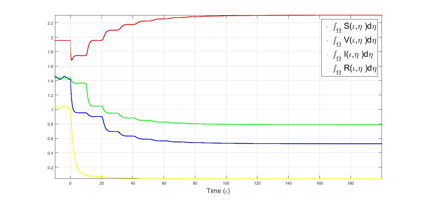
Here, we validate our theoretical results by numerical simulation. We set $\Omega=(-1,1)$ and

J(\eta)=\begin{cases}2.2523e^{\frac{1}{\eta^{2}-1}},&-1<\eta<1,\\ 0,&\text{otherwise}.\end{cases}

This ensures that

\int_{\mathbb{R}}J(\eta)\,d\eta\approx 1,

and that assumptions (P0) and (P1) are fulfilled.

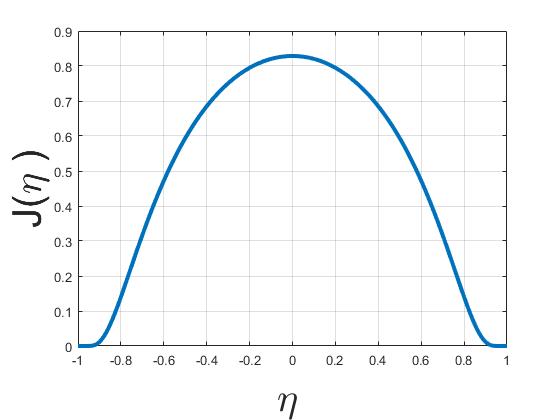
Refer to caption — Figure 1. Kernel function $J$ .

We consider the following set of parameters:

$\displaystyle\mu$	$\displaystyle=10^{-1},$	$\displaystyle\beta_{S}(\eta)$	$\displaystyle=15\cdot 10^{-1},$	$\displaystyle\beta_{V}(\eta)$	$\displaystyle=12\cdot 10^{-1},$	$\displaystyle\beta_{I}(\eta)$	$\displaystyle=13\cdot 10^{-1},$
$\displaystyle\lambda_{1}(\eta)$	$\displaystyle=29\cdot 10^{-1},$	$\displaystyle\tau_{V}$	$\displaystyle=98\cdot 10^{-1},$	$\displaystyle\beta(\eta)$	$\displaystyle=\bar{\beta},$	$\displaystyle\alpha(\eta)$	$\displaystyle=1,$
$\displaystyle K_{I}$	$\displaystyle=5\cdot 10^{-2},$	$\displaystyle\zeta$	$\displaystyle=98\cdot 10^{-1}.$

	$\displaystyle S_{0}(\iota,\eta)$	$\displaystyle=3\cdot 10^{-1}+5\cdot 10^{-2}\cos(\eta),$
	$\displaystyle V_{0}(\iota,\eta)$	$\displaystyle=41\cdot 10^{-2}+10^{-2}\cos(\eta)+10^{-3}\cos(\iota),$
	$\displaystyle I_{0}(\iota,\eta)$	$\displaystyle=71\cdot 10^{-2}+10^{-1}\cos(\eta)+10^{-2}\cos(3\iota).$

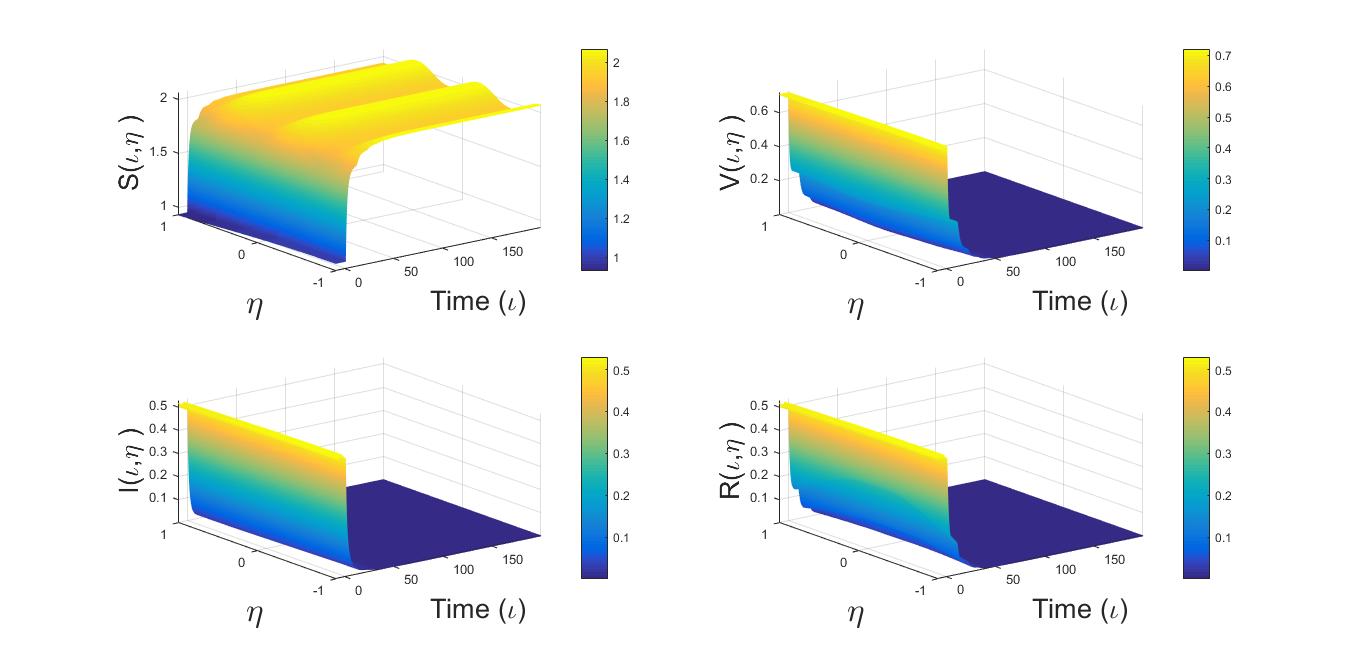
First, we take $\bar{\beta}=47\cdot 10^{-2}$ . Then $\mathcal{R}_{0}=0.7614<1$ , and the infection-free steady state $H_{0}$ is globally asymptotically stable; see Figure 2.

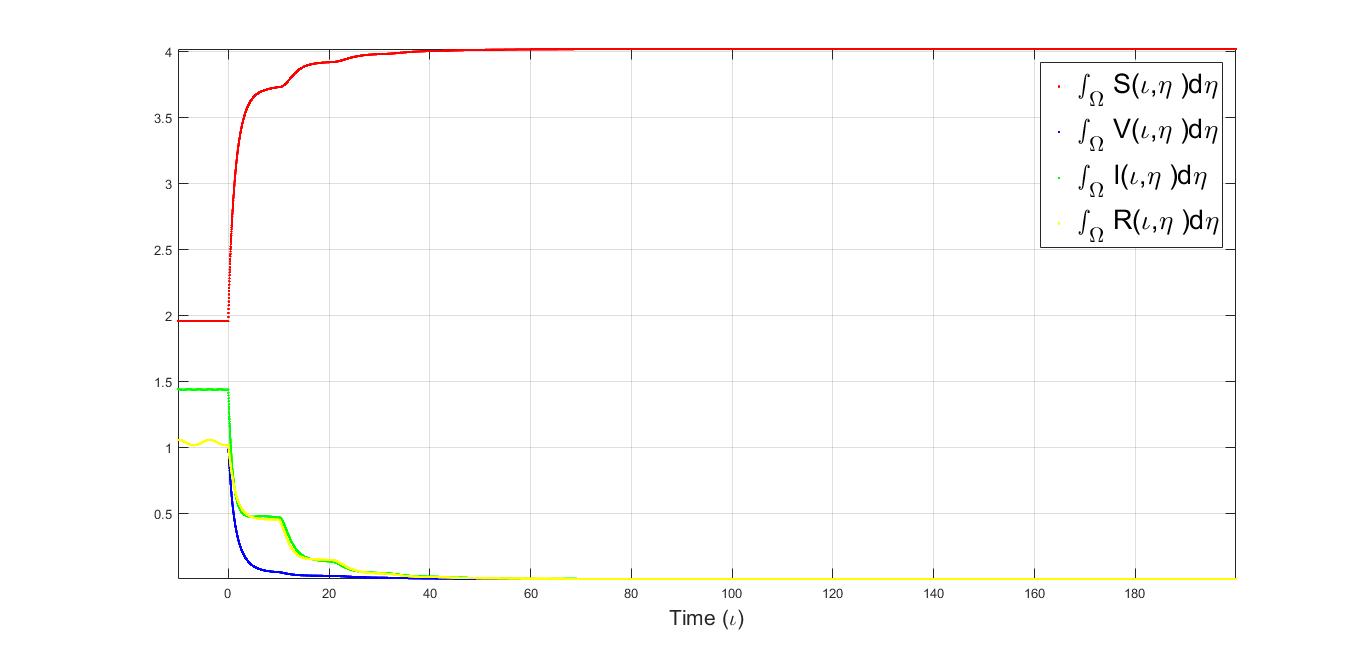
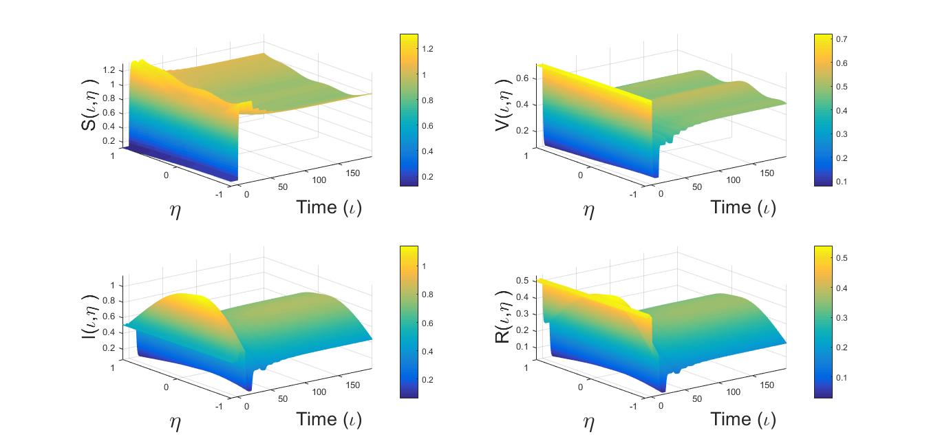
Next, the immunity-free infected steady state $H_{1}$ is globally asymptotically stable for $\bar{\beta}=23\cdot 10^{-2}$ and $\beta_{R}(\eta)=187\cdot 10^{-1}$ , where $\mathcal{R}_{0}=3.5874>1$ and $\mathcal{R}_{1}=0.3956<1$ ; see Figure 3.

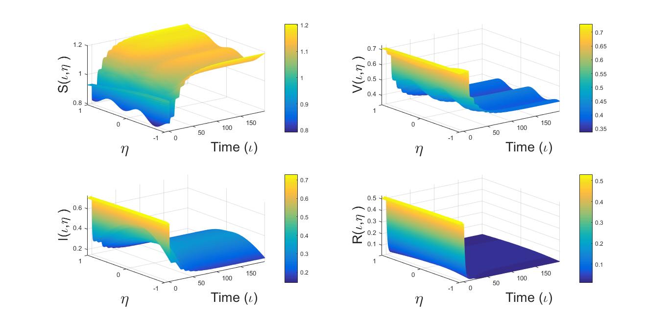
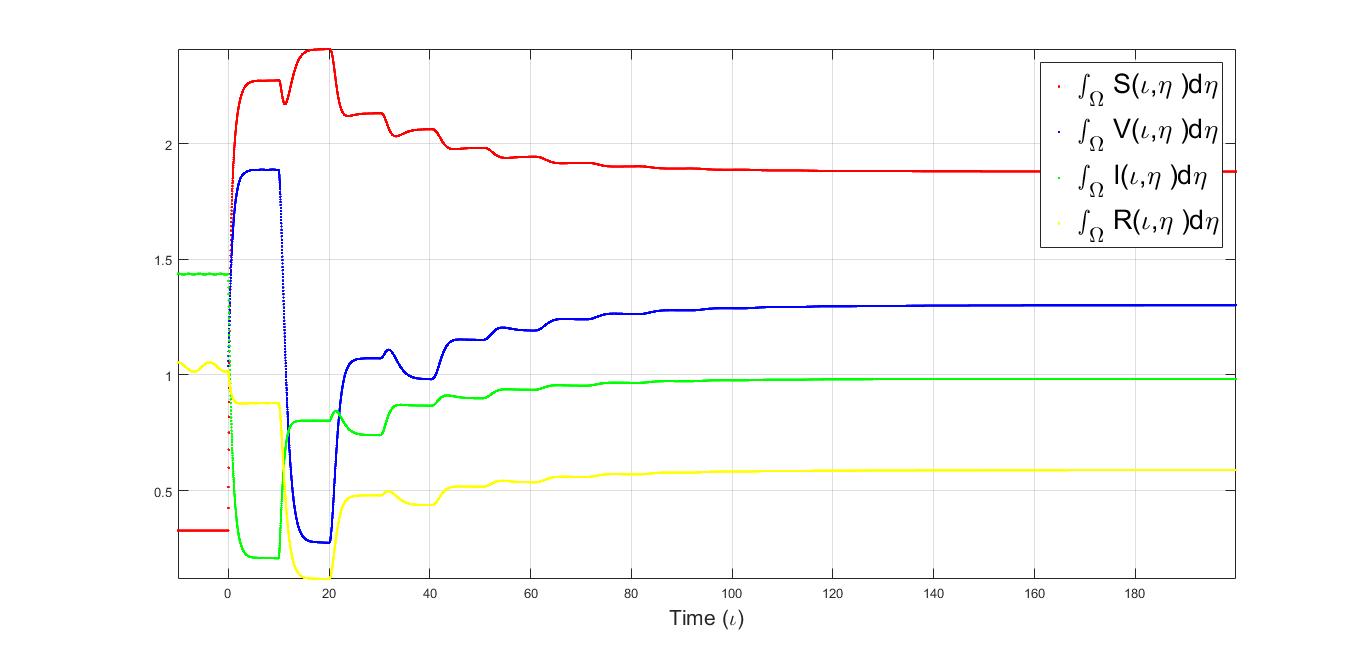
Finally, for $\beta_{R}(\eta)=53\cdot 10^{-1}$ and $\mathcal{R}_{1}=2.1894>1$ , the infected-immune steady state $H_{2}$ is globally asymptotically stable; see Figure 4.

9. Conclusions

This paper presents and examines a model of nonlocal dispersal viral infection that includes humoral immunity, intracellular delay, and transmissions from virus to cell as well as cell to cell.

We have proved that the global dynamics of system (2)–(3) is determined by the basic reproduction number of infection $\Re_{0}$ and the basic reproduction number of immunity $\Re_{1}$ . By analyzing the characteristic equations and constructing Lyapunov functionals, we have obtained the following conclusions: if $\Re_{0}<1$ , then the infection-free steady state $H_{0}$ is globally asymptotically stable; if $\Re_{1}\leqslant 1<\Re_{0}$ , then the immunity-free infected steady state $H_{1}$ is globally asymptotically stable. We note that constructing a Lyapunov functional for a delayed nonlocal diffusive problem is not straightforward.

Additionally, using a set of assertions that confirm every assumption of Theorem 3 in [18], we demonstrated the system’s uniform persistence. As a result, the semiflow $\Xi(\iota)$ is uniformly persistent, and the system admits at least one positive steady state. Finally, we supported our findings using graphical representations.

References

[1] M.A. Nowak, C.R.M. Bangham, Population dynamics of immune responses to persistent viruses, Science, 272 (1996), pp. 74–79.
[2] J. Lin, R. Xu, X. Tian, Threshold dynamics of an HIV-1 virus model with both virus-to-cell and cell-to-cell transmissions, intracellular delay, and humoral immunity, Appl. Math. Comput., 315 (2017), pp. 516–530.
[3] J. Garcia-Melian, J.D. Rossi, On the principal eigenvalue of some nonlocal diffusion problems, J. Differential Equations, 246 (2009), pp. 21–38.
[4] K.J. Engel and R. Nagel, One-Parameter Semigroups for Linear Evolution Equations, Graduate Texts in Mathematics, Springer, New York, 2000.
[5] A. Pazy, Semigroups of Linear Operators and Applications to Partial Differential Equations, Springer, New York, 1983.
[6] S. Han and C. Lei, Stability of equilibria of a diffusive SEIR epidemic model with nonlinear incidence, Appl. Math. Lett., 98 (2019), pp. 114–120.
[7] G. Webb, Theory of Nonlinear Age-Dependent Population Dynamics, CRC Press, 1985.
[8] F.Y. Yang and W.T. Li, Dynamics of a nonlocal dispersal SIS epidemic model, Commun. Pure Appl. Anal., 16 (2017), p. 781.
[9] K. Allali, S. Harroudi, D.F.M. Torres, Analysis and optimal control of an intracellular delayed HIV model with CTL immune response, J. Math. Comput. Sci., 12 (2018), pp. 111–127.
[10] G. Zhao and S. Ruan, Spatial and temporal dynamics of a nonlocal viral infection model, SIAM J. Appl. Math., 78 (2018) no. 4, pp. 1954–1980.
[11] J.K. Hale, Asymptotic Behavior of Dissipative Systems, Mathematical Surveys and Monographs, vol. 25, American Mathematical Society, Providence, RI, 1988.
[12] P. Magal and X.Q. Zhao, Global attractors and steady states for uniformly persistent dynamical systems, SIAM J. Math. Anal., 37 (2005) no. 1, pp. 251–275.
[13] H.R. Thieme, Spectral bound and reproduction number for infinite-dimensional population structure and time heterogeneity, SIAM J. Math. Anal., 70 (2009), pp. 188–211.
[14] X.Q. Zhao, Dynamical Systems in Population Biology, vol. 16, Springer, New York, 2017.
[15] A.M. Elaiw, A.A. Raezah, K. Hattaf, Stability of HIV-1 infection with saturated virus-target and infected-target incidences and CTL immune response, Int. J. Biomath., 10 (2017), 1750070.
[16] W. Desch and W. Schappacher, Linearized stability for nonlinear semigroups, in Differential Equations in Banach Spaces, Lecture Notes in Mathematics, A. Favini and E. Obrecht (eds.), Springer-Verlag, Berlin, Heidelberg, 1986, pp. 61–67.
[17] K. Hattaf and N. Yousfi, A generalized HBV model with diffusion and two delays, Comput. Math. Appl., 69 (2015), pp. 31–40.
[18] H.L. Smith and X.Q. Zhao, Robust persistence for semidynamical systems, Nonlinear Anal., 47 (2001) no. 9, pp. 6169–6179.
[19] W. Shen and A. Zhang, Spreading speeds for monostable equations with nonlocal dispersal in space periodic habitats, J. Differential Equations, 249 (2010) no. 4, pp. 747–795.
[20] W. Wang and X.Q. Zhao, Basic reproduction numbers for reaction–diffusion epidemic models, SIAM J. Appl. Dyn. Syst., 11 (2012), pp. 1652–1673.
[21] C. Qin, Y. Chen, X. Wang, Global dynamics of a delayed diffusive virus infection model with cell-mediated immunity and cell-to-cell transmission, Math. Biosci. Eng., 17 (2020) no. 5, pp. 4678–4705.
[22] Y. Yang, T. Zhang, J. Zhou, Global attractivity of a time-delayed viral infection model with spatial heterogeneity, Appl. Math. Lett., 116 (2021), 107035.
[23] S. Djilali, Threshold asymptotic dynamics for a spatial age-dependent cell-to-cell transmission model with nonlocal dispersal, Discrete Contin. Dyn. Syst., 28 (2023) no. 7, pp. 4108–4143.
[24] L. Liu, R. Xu, Z. Jin, Global dynamics of a spatial heterogeneous viral infection model with intracellular delay and nonlocal diffusion, Appl. Math. Model., 82 (2020), pp. 150–167.

This work is licensed under a Creative Commons Attribution 4.0 International License.

		$\displaystyle\\|V(\iota;.)\\|\leq$
		$\displaystyle\leq e^{-\beta_{V}\iota}\\|V_{0}\\|$
		$\displaystyle\quad+\int\limits_{0}^{\iota}e^{-\beta_{V}(\iota-\sigma)}e^{-\mu\tau_{V}}\\|S(\sigma-\tau_{v},\cdot)\\|(\\|\beta\\|\\|I(\sigma-\tau_{v},\cdot)\\|+\\|\alpha\\|\\|V(\sigma-\tau_{v},\cdot)\\|)d\sigma,$
		$\displaystyle\leq e^{-\beta_{V}\iota}\\|V_{0}\\|+Ke^{-\mu\tau_{V}}\int\limits_{0}^{\iota}e^{-\beta_{V}(\iota-\sigma)}(\\|\beta\\|\\|I(\sigma-\tau_{v},\cdot)\\|+\\|\alpha\\|\\|V(\sigma-\tau_{v},\cdot)\\|)d\sigma,$
		$\displaystyle\leq e^{-\beta_{V}\iota}\\|V_{0}\\|+K\beta^{\ast}e^{-\mu\tau_{V}}\int\limits_{0}^{\iota}e^{-\beta_{V}(\iota-\sigma)}(\\|I(\sigma-\tau_{v},\cdot)\\|+\\|V(\sigma-\tau_{v},\cdot)\\|)d\sigma,$

		$\displaystyle\\|V(\iota,\cdot)\\|\leq$
		$\displaystyle\leq e^{-\beta_{V}\iota}\\|V_{0}\\|+K\beta^{\ast}e^{-\mu\tau_{V}}\int\limits_{\tau_{v}}^{\iota-\tau_{v}}e^{-\beta_{V}(\iota-\tau_{v}-\sigma)}(\\|I(\sigma,\cdot)\\|+\\|V(\sigma,\cdot)\\|)d\sigma$
		$\displaystyle\leq e^{-\beta_{V}\iota}\\|V_{0}\\|+K\beta^{\ast}e^{-\mu\tau_{V}}\int\limits_{\tau_{v}}^{\iota-\tau_{v}}e^{-\beta_{V}(\iota-\tau_{v}-\sigma)}\\|V(\sigma,\cdot)\\|d\sigma$
		$\displaystyle\quad+K\beta^{\ast}e^{-\mu\tau_{V}}\int\limits_{\tau_{v}}^{\iota-\tau_{v}}e^{-\beta_{V}(\iota-\tau_{v}-\sigma)}\\|I(\sigma,\cdot)\\|d\sigma.$

		$\displaystyle\\|V(\iota,\cdot)\\|\leq$
		$\displaystyle\leq e^{-\beta_{V}\iota}\\|V_{0}\\|+K\beta^{\ast}e^{-\mu\tau_{V}}\int\limits_{\tau_{v}}^{\iota-\tau_{v}}e^{-\beta_{V}(\iota-\tau_{v}-\sigma)}\\|V(\sigma,\cdot)\\|d\sigma$
		$\displaystyle\quad+K\beta^{\ast}e^{-\mu\tau_{V}}\int\limits_{\tau_{v}}^{\iota-\tau_{v}}e^{-\beta_{V}(\iota-\tau_{v}-\sigma)}\left\{e^{-\lambda\sigma}\\|I_{0}\\|+\\|\beta_{1}\\|_{0}^{\sigma}e^{-\lambda(\sigma-s)}\\|V(s,\cdot)\\|ds\right\}d\sigma$
		$\displaystyle\leq e^{-\beta_{V}\iota}\\|V_{0}\\|+K\beta^{\ast}e^{-\mu\tau_{V}}\int\limits_{\iota_{v}}^{\iota-\tau_{v}}e^{-\beta_{V}(\tau-\tau_{v}-\sigma)}\\|V(\sigma,\cdot)\\|d\sigma$
		$\displaystyle\quad+K\beta^{\ast}e^{-\mu\tau_{V}}\\|I_{0}\\|\int\limits_{-\tau_{v}}^{\iota-\tau_{v}}e^{-\beta_{V}(\iota-\tau_{v}-\sigma)}e^{-\lambda\sigma}d\sigma$
		$\displaystyle\quad+\\|\beta_{1}\\|K\beta^{\ast}e^{-\mu\tau_{V}}\int\limits_{-\tau_{v}}^{\iota-\tau_{v}}e^{-\beta_{V}(\iota-\tau_{v}-\sigma)}\int\limits_{-\tau_{v}}^{\sigma}e^{-\lambda(\sigma-s)}\\|V(s,\cdot)\\|dsd\sigma$
		$\displaystyle\leq e^{-\beta_{V}\iota}\\|V_{0}\\|+K\beta^{\ast}e^{-\mu\tau_{V}}\int\limits_{-\tau_{v}}^{\iota-\tau_{v}}e^{-\beta_{V}(\tau-\tau_{v}-\sigma)}\\|V(\sigma,\cdot)\\|d\sigma$
		$\displaystyle\quad+K\beta^{\ast}e^{-\mu\tau_{V}}\\|I_{0}\\|\int\limits_{-\tau_{v}}^{\iota-\tau_{v}}e^{-\lambda\sigma}d\sigma$
		$\displaystyle\quad+\\|\beta_{1}\\|M\beta^{\ast}e^{-\mu\tau_{V}}\int\limits_{-\tau_{v}}^{\iota-\tau_{v}}e^{-\beta_{V}(\iota-\tau_{v}-\sigma)}\int\limits_{-\tau_{v}}^{\sigma}e^{-\lambda(\sigma-s)}\\|V(s,.)\\|dsd\sigma.\text{ }$

		$\displaystyle\\|V(\iota,\cdot)\\|\leq$
		$\displaystyle\leq e^{-\beta_{V}\iota}\\|V_{0}\\|+K\beta^{\ast}e^{-\mu\tau_{V}}\int\limits_{-\tau_{v}}^{\iota-\tau_{v}}e^{-\beta_{V}(\tau-\tau_{v}-\sigma)}\\|V(\sigma,\cdot)\\|d\sigma$
		$\displaystyle\quad+K\beta^{\ast}e^{-\mu\tau_{V}}\\|I_{0}\\|\tfrac{e^{\lambda\tau_{v}}-e^{-\lambda(\iota-\tau_{v})}}{\lambda}$
		$\displaystyle\quad+\\|\beta_{1}\\|K\beta^{\ast}e^{-\mu\tau_{V}}e^{-\beta_{V}(\iota-\tau_{v})}\int\limits_{-\tau_{v}}^{\iota-\tau_{v}}e^{\lambda s}\\|V(s,\cdot)\\|\int\limits_{s}^{\iota-\tau_{v}}e^{(\beta_{V}-\lambda)\sigma}d\sigma ds$
		$\displaystyle\leq e^{-\beta_{V}\tau}\\|V_{0}\\|+K\beta^{\ast}e^{-\mu\tau_{V}}\int\limits_{-\tau_{v}}^{\iota-\tau_{v}}e^{-\beta_{V}(\tau-\tau_{v}-\sigma)}\\|V(\sigma,\cdot)\\|d\sigma$
		$\displaystyle\quad+K\beta^{\ast}e^{-\mu\tau_{V}}\\|I_{0}\\|\tfrac{e^{\lambda\tau_{v}}-e^{-\lambda(\iota-\tau_{v})}}{\lambda}$
		$\displaystyle\quad+\\|\beta_{1}\\|K\beta^{\ast}e^{-\mu\tau_{V}}\tfrac{e^{-\varpi(\tau-\tau_{v})}}{\lambda-\beta_{V}}\int\limits_{-\tau_{v}}^{\iota-\tau_{v}}e^{\varpi s}\\|V(s,\cdot)\\|ds$
		$\displaystyle\leq\\|V_{0}\\|+K\beta^{\ast}e^{-\mu\tau_{V}}\int\limits_{-\tau_{v}}^{\iota-\tau_{v}}e^{-\varpi(\tau-\tau_{v}-\sigma)}\\|V(\sigma,\cdot)\\|d\sigma$
		$\displaystyle\quad+K\beta^{\ast}e^{-\mu\tau_{V}}\\|I_{0}\\|\tfrac{e^{\lambda\tau_{v}}}{\lambda}$
		$\displaystyle\quad+\tfrac{\\|\beta_{1}\\|K\beta^{\ast}e^{-\mu\tau_{V}}}{\lambda-\beta_{V}}\int\limits_{-\tau_{v}}^{\iota-\tau_{v}}e^{-\varpi(\iota-\tau_{v}-s)}\\|V(s,\cdot)\\|ds$
		$\displaystyle\leq C_{1}+C_{2}\int\limits_{-\tau_{v}}^{\iota-\tau_{v}}\\|V(s,\cdot)\\|ds,$

	$\displaystyle\\|I(\iota,\cdot)\\|$	$\displaystyle\leq\\|I_{0}\\|+\tfrac{C_{1}\\|\beta_{1}\\|e^{C_{2}\iota}}{\lambda}=C_{3},$
	$\displaystyle\\|I(\iota,\cdot)\\|$	$\displaystyle\leq\\|I_{0}\\|e^{-\lambda\iota}+\\|\beta_{1}\\|\int_{0}^{\iota}e^{-\lambda(\iota-\sigma)}\\|V(\sigma,\cdot)\\|d\sigma$
		$\displaystyle\leq\\|I_{0}\\|e^{-\lambda\iota}+C_{1}\\|\beta_{1}\\|\int_{0}^{\iota}e^{-\lambda(\iota-\sigma)}e^{C_{2}\iota}d\sigma$
		$\displaystyle\leq\\|I_{0}\\|+\tfrac{C_{1}\\|\beta_{1}\\|e^{C_{2}\iota}}{\lambda}=C_{3}.$

Abstract.

Key words and phrases:

2005 Mathematics Subject Classification

1. Introduction

2. Preliminaries

Lemma .

Proof.

Theorem 1.

Proof.

Theorem 2.

Proof.

3. Compactness

Lemma .

Proof.

Lemma .

Proof.

Lemma .

Proof.

4. Basic reproduction number and steady-state

Lemma .

Proof.

Lemma .

5. Extinction scenario of virus

Theorem 3.

Proof.

Lemma .

Proof.

Remark .

Theorem 4.

Proof.

6. Uniform persistence

Theorem 5.

Proof.

Claim .

Claim .

Claim .

Claim .

7. Global behavior analysis

Theorem 6.

Proof.

8. Graphical representation

9. Conclusions

References

Information

Indexing and abstracting

Publisher