An Ushijima-Type Analysis for the Numerical Blow-up of a Fractional Reaction-Diffusion EquationThanks: Université Nangui Abrogoua, Abidjan, Côte d’Ivoire, e-mail: yekreben@gmail.com (Corresponding author), ORCID: 0009-0008-7508-3644 .Thanks: Université Nangui Abrogoua, Abidjan, Côte d’Ivoire, e-mail: kra.amaniyeh@gmail.com, ORCID: 0009-0007-4693-2814 .Thanks: Université Nangui Abrogoua, Abidjan, Côte d’Ivoire, e-mail: halimanachid@yahoo.fr, ORCID: 0000-0003-1244-8139 .

Abstract.

This paper studies the blow-up phenomenon for a nonlinear reaction-diffusion equation with a Caputo fractional time derivative. Our work has two main parts. First, we prove that the solution of the semi-discretized system blows up in a finite time $T_h$ if the initial data is large enough. Second, we analyze the full discretization using the explicit L1 scheme. By introducing a discrete weighted functional and comparing it to an auxiliary sequence, we show that the numerical solution also blows up in finite time, provided we use an adaptive time-stepping strategy. The main contribution of this work is to show that our lemmas provide the necessary tools to apply Ushijima’s theoretical framework to this class of fractional problems. This builds a bridge between Ushijima’s theory and non-local fractional schemes. We can then conclude that the numerical blow-up time converges to the semi-discrete one, which validates the ability of the scheme to capture the singularity dynamics.

1. Introduction

The numerical capture of finite-time blow-up in nonlinear reaction-diffusion equations is a major challenge in modern numerical analysis. The problem is not only to show that the numerical solution grows to infinity, but to ensure that the numerical blow-up time converges to the continuous one. For classical parabolic equations, this is well understood. However, time-fractional derivatives of Caputo type change the situation: they introduce a non-local memory effect that makes standard analysis methods difficult to use.

Following the work of Ushijima [22], a strict methodology was created to prove the convergence of blow-up time for local parabolic equations. More recently, Wang et al. [24] studied the L1 scheme for fractional ordinary differential equations (FODE). However, there is still a gap for fractional partial differential equations (FPDE), where we must manage both the temporal non-locality and the spatial diffusion operator. The Ushijima framework was not designed for memory operators, and the approach by Wang does not include the complex interactions caused by the Laplacian.

This work aims to fill this gap by studying the following fractional reaction-diffusion equation (S):

(1)

where $\beta \in (0,1)$ and $p>1$. Our study focuses on solving three main difficulties:

First, we establish the blow-up proof for the semi-discretized system. The challenge is to maintain positivity and growth while considering both the discrete Laplacian and the Caputo memory. We solve this by using a fractional extremum principle combined with weighted functionals.

Second, we deal with the complexity of the full discretization using the explicit L1 scheme. Managing non-locality on an adaptive time mesh which is necessary to approach the singularity makes the analysis of memory weights very difficult. Our solution is based on constructing an auxiliary comparison sequence and using a discrete Jensen inequality. This guarantees the existence of numerical blow-up where standard uniform mesh analysis often fails.

Finally, and this is our most important contribution, we demonstrate that this numerical blow-up satisfies the critical condition A0 of the Ushijima framework. Unlike previous studies that only observe the blow-up, we build an original theoretical bridge between Ushijima’s theory and non-local fractional schemes. By validating this connection, we do more than just simulate a singularity; we create the foundation to prove, in future work, the rigorous convergence of the numerical blow-up time. This confirms that our scheme captures the true essence of the singular dynamics.

2. Semi-discretization and blow-up

We begin by discretising problem (1) in space only. Let $I$ be a positive integer, $h=1/I$ the spatial step size, and $x_i=ih$ for $i=0,\mathrm{\dots },I$. Let $U_i(t)$ be an approximation of $u(x_i,t)$. By replacing the second spatial derivative with a centred finite difference, we obtain the system of fractional ordinary differential equations (FODE):

(2) ${}_t{}^{}{}_{}{}^{C}D_{}^{\beta }{U}_i(t)$ $\phantom{}=D{\delta }^2{U}_i(t)+{[U_i(t)]}^p,$ $i=1,\mathrm{\dots },I-1,$

(3) $U_0(t)$ $\phantom{}=U_I(t)=0,$ $t\ge 0,$

(4) $U_i(0)$ $\phantom{}=u_0(x_i),$ $i=0,\mathrm{\dots },I,$

where ${\delta }^2$ is the discrete Laplacian operator: ${\delta }^2{U}_i(t)=(U_{i+1}(t)-2U_i(t)+U_{i-1}(t))/h^2$.

The analysis of this system is based on the associated eigenvalue problem ${\delta }^2({\mathrm{\Phi }}_{k,i})=-{\lambda }_{k,h}{\mathrm{\Phi }}_{k,i}$ with zero Dirichlet boundary conditions. The eigenvalues and eigenvectors are well known:

(5) ${\lambda }_{k,h}$ $=\frac{2(1-\cos (k\pi h))}{h^2},k=1,\mathrm{\dots },I-1,$

(6) ${\mathrm{\Phi }}_{k,i}$ $=\sin (ki\pi h),i=0,\mathrm{\dots },I.$

The first eigenvector ${\mathrm{\Phi }}_1$, associated with the first eigenvalue ${\lambda }_{1,h}$, has components ${\mathrm{\Phi }}_{1,i}=\sin (i\pi h)$ that are strictly positive for $i=1,\mathrm{\dots },I-1$.

2.1. Blow-up of the Semi-Discrete Solution

To study the behavior of the solution $U_i(t)$, we introduce a weighted functional.

Definition .

The weighted functional $J_{\mathrm{\Phi },h}(t)$ is defined by:

$$J_{\mathrm{\Phi },h}(t)=h\sum _{j=1}^{I-1}{U}_j(t){\mathrm{\Phi }}_{1,j}.$$

The initial condition $u_0(x)$ is chosen such that $J_{\mathrm{\Phi },h}(0)>0$.

Our analysis is based on the following results.

Lemma (Non-negativity of the solution).

Let $U_i(t)$ be the solution of the system (2)–(4) with $u_0(x)\ge 0$ and $u_0\not\equiv 0$. Then, $U_i(t)>0$ for all $i\in \{1,\mathrm{\dots },I-1\}$ and for all $t\in (0,T_{max})$, where $T_{max}$ is the maximum existence time.

Proof.

Suppose that there exists a first time $t_0>0$ and an index $k_0\in \{1,\mathrm{\dots },I-1\}$ such that $U_{k_0}(t_0)=0$ and $U_i(t)\ge 0$ for all $i$ and $t\in [0,t_0]$. Since $U_{k_0}(t_0)=0$ is a minimum for $U_{k_0}(t)$ on the interval $[0,t_0]$, the extremum principle for the Caputo derivative (see [25], Theorem 3.2) implies:

(7) $${}_t{}^{}{}_{}{}^{C}D_{}^{\beta }{U}_{k_0}(t_0)\le \frac{-U_{k_0}(0)}{\mathrm{\Gamma }(1-\beta )t_0^{\beta }}\le 0.$$

On the other hand, from the governing equation (2) at $t=t_0$, we have:

$${}_t{}^{}{}_{}{}^{C}D_{}^{\beta }{U}_{k_0}(t_0)=D\frac{U_{k_0-1}(t_0)-2U_{k_0}(t_0)+U_{k_0+1}(t_0)}{h^2}+{[U_{k_0}(t_0)]}^p.$$

Substituting $U_{k_0}(t_0)=0$, we obtain:

$${}_t{}^{}{}_{}{}^{C}D_{}^{\beta }{U}_{k_0}(t_0)=D\frac{U_{k_0-1}(t_0)+U_{k_0+1}(t_0)}{h^2}\ge 0,$$

since $U_{k_0\pm 1}(t_0)\ge 0$. Comparing with (7), we must have ${}_t{}^{}{}_{}{}^{C}D_{}^{\beta }{U}_{k_0}(t_0)=0$, which implies $U_{k_0\pm 1}(t_0)=0$ and $U_{k_0}(0)=0$. By propagation to all neighbors, we find $U_i(0)=0$ for all $i$, which contradicts the assumption $u_0\not\equiv 0$. Therefore, the assumption that the solution touches zero is false, and we conclude $U_i(t)>0$ for all $t\in (0,T_{max})$. ∎

Lemma (Weighted Discrete Jensen’s Inequality).

Let $\zeta :ℝ\to ℝ$ be a convex function. Let $x_1,\mathrm{\dots },x_N\in ℝ$ and ${\omega }_1,\mathrm{\dots },{\omega }_N$ be non-negative weights such that $S_{\omega }={\sum }_{j=1}^N{\omega }_j>0$. Then:

$$\frac{1}{S_{\omega }}\sum _{j=1}^N{\omega }_j\zeta (x_j)\ge \zeta \left(\frac{1}{S_{\omega }}\sum _{j=1}^N{\omega }_j{x}_j\right).$$

Proposition .

The functional $J_{\mathrm{\Phi },h}(t)$ satisfies the following fractional differential inequality:

(8) $${}_t{}^{}{}_{}{}^{C}D_{}^{\beta }{J}_{\mathrm{\Phi },h}(t)\ge -D{\lambda }_{1,h}{J}_{\mathrm{\Phi },h}(t)+K_{p,h}{[J_{\mathrm{\Phi },h}(t)]}^p,$$

where the constant $K_{p,h}$ is defined by $K_{p,h}={\left(h{\displaystyle \sum _{j=1}^{I-1}}{\mathrm{\Phi }}_{1,j}\right)}^{1-p}$.

Proof.

Applying the operator ${}_t{}^{}{}_{}{}^{C}D_{}^{\beta }$ to $J_{\mathrm{\Phi },h}(t)$ and using equation (2), we have:

${}_t{}^{}{}_{}{}^{C}D_{}^{\beta }{J}_{\mathrm{\Phi },h}(t)$ $\phantom{}=h{\displaystyle \sum _{j=1}^{I-1}}({}_t{}^{}{}_{}{}^{C}D_{}^{\beta }{U}_j(t)){\mathrm{\Phi }}_{1,j}$

$\phantom{}=h{\displaystyle \sum _{j=1}^{I-1}}(D{\delta }^2{U}_j(t)+{[U_j(t)]}^p){\mathrm{\Phi }}_{1,j}$

$\phantom{}=D\left(h{\displaystyle \sum _{j=1}^{I-1}}({\delta }^2{U}_j(t)){\mathrm{\Phi }}_{1,j}\right)+h{\displaystyle \sum _{j=1}^{I-1}}{[U_j(t)]}^p{\mathrm{\Phi }}_{1,j}.$

Using the symmetry property of ${\delta }^2$ and the fact that ${\mathrm{\Phi }}_1$ is an eigenvector, the diffusion term becomes:

$h{\displaystyle \sum _{j=1}^{I-1}}({\delta }^2{U}_j(t)){\mathrm{\Phi }}_{1,j}$ $\phantom{}=h{\displaystyle \sum _{j=1}^{I-1}}{U}_j(t)({\delta }^2{\mathrm{\Phi }}_{1,j})=-{\lambda }_{1,h}\left(h{\displaystyle \sum _{j=1}^{I-1}}{U}_j(t){\mathrm{\Phi }}_{1,j}\right)=-{\lambda }_{1,h}{J}_{\mathrm{\Phi },h}(t).$

For the nonlinear term, Section 2.1 guarantees that $U_j(t)\ge 0$. The function $\zeta (x)=x^p$ is convex for $x\ge 0$ since $p>1$. We apply Section 2.1 with $x_j=U_j(t)$ and ${\omega }_j={\mathrm{\Phi }}_{1,j}>0$. Let $S_{\omega }={\sum }_{j=1}^{I-1}{\mathrm{\Phi }}_{1,j}$.

$h{\displaystyle \sum _{j=1}^{I-1}}{[U_j(t)]}^p{\mathrm{\Phi }}_{1,j}$ $\phantom{}=h{S}_{\omega }\left({\displaystyle \frac{1}{S_{\omega }}}{\displaystyle \sum _{j=1}^{I-1}}{\mathrm{\Phi }}_{1,j}{[U_j(t)]}^p\right)$

$\phantom{}\ge h{S}_{\omega }{\left({\displaystyle \frac{1}{S_{\omega }}}{\displaystyle \sum _{j=1}^{I-1}}{\mathrm{\Phi }}_{1,j}{U}_j(t)\right)}^p$

$\phantom{}=h{S}_{\omega }{\displaystyle \frac{{\left(\sum {\mathrm{\Phi }}_{1,j}{U}_j(t)\right)}^p}{{(S_{\omega })}^p}}={\displaystyle \frac{h{\left(h\sum {\mathrm{\Phi }}_{1,j}{U}_j(t)\right)}^p}{h^p{(S_{\omega })}^{p-1}}}$

$\phantom{}={\displaystyle \frac{{[J_{\mathrm{\Phi },h}(t)]}^p}{{(h{S}_{\omega })}^{p-1}}}={\left(h{\displaystyle \sum _{j=1}^{I-1}}{\mathrm{\Phi }}_{1,j}\right)}^{1-p}{[J_{\mathrm{\Phi },h}(t)]}^p.$

Combining the two terms, we obtain the inequality (8). ∎

Theorem 1 (Blow-up of the Semi-Discrete Solution).

Assume $p>1$. If the initial condition $u_0(x)$ is such that the weighted functional $J(0)\equiv J_{\mathrm{\Phi },h}(0)$ satisfies:

(9) $$J(0)>{\left(\frac{D{\lambda }_{1,h}}{K_{p,h}}\right)}^{\frac{1}{p-1}}≕J_{\mathrm{crit}},$$

then the solution $U_i(t)$ of the semi-discrete system (2)–(4) blows up in finite time . Moreover, the blow-up time satisfies the upper bound [15, Corollary 2]:

(10)

Proof.

By Section 2.1, the weighted functional $J(t)$ satisfies the fractional differential inequality:

(11) $${}_t{}^{}{}_{}{}^{C}D_{}^{\beta }J(t)\ge K_{p,h}J{(t)}^p-D{\lambda }_{1,h}J(t)≕f(J(t)),$$

with initial condition $J(0)>J_{\mathrm{crit}}={\left(\frac{D{\lambda }_{1,h}}{K_{p,h}}\right)}^{\frac{1}{p-1}}$.

Since $J(t)\ge J(0)>J_{\mathrm{crit}}$ (by strict positivity of the fractional derivative when $f(J(0))>0$), and the function $\varphi (u)=K_{p,h}-D{\lambda }_{1,h}{u}^{-(p-1)}$ is increasing on $[J_{\mathrm{crit}},\mathrm{\infty })$, we have for all $t\ge 0$:

(12) $$f(J(t))\ge \left(K_{p,h}-D{\lambda }_{1,h}J{(0)}^{-(p-1)}\right)J{(t)}^p=C^{\ast }J{(t)}^p,$$

where $C^{\ast }=\frac{K_{p,h}J{(0)}^{p-1}-D{\lambda }_{1,h}}{J{(0)}^{p-1}}>0$ by hypothesis on $J(0)$.

By the equivalence between the Caputo differential inequality and the Volterra integral formulation [4, Theorem 3.1], we obtain:

(13) $$J(t)\ge J(0)+\frac{C^{\ast }}{\mathrm{\Gamma }(\beta )}{\int }_0^t{(t-s)}^{\beta -1}J{(s)}^p𝑑s.$$

Consider the candidate subsolution $\underset{¯}{y}(t)=J(0){\left(1-\frac{t}{T}\right)}^{-q}$ defined on $[0,T)$ with $q=\frac{\beta }{p-1}>0$. This function satisfies $\underset{¯}{y}(0)=J(0)$ and $\underset{t\to T^{-}}{lim}\underset{¯}{y}(t)=+\mathrm{\infty }$.

For $\underset{¯}{y}$ to be a subsolution of (13), it suffices that:

(14) $$\underset{¯}{y}(t)\le J(0)+\frac{C^{\ast }}{\mathrm{\Gamma }(\beta )}{\int }_0^t{(t-s)}^{\beta -1}\underset{¯}{y}{(s)}^p𝑑s≕I(t).$$

By the substitution $s=t-(T-t)\sigma$ and using $pq=\beta +q$, one computes:

(15) ${\displaystyle {\int }_0^t}{(t-s)}^{\beta -1}{\left(1-\frac{s}{T}\right)}^{-pq}𝑑s=T^{\beta +q}{(T-t)}^{-q}B(\frac{t}{T-t},\beta ,q),$

where $B(x,\beta ,q)={\int }_0^x{\sigma }^{\beta -1}{(1+\sigma )}^{-(\beta +q)}𝑑\sigma$ is the incomplete Beta function [4, Chapter 6].

As $t\to T^{-}$, $B(x,\beta ,q)\to \frac{\mathrm{\Gamma }(\beta )\mathrm{\Gamma }(q)}{\mathrm{\Gamma }(\beta +q)}$, so the dominant behavior of $I(t)$ near $T$ is:

(16) $$I(t)\sim J(0)+\frac{C^{\ast }J{(0)}^p\mathrm{\Gamma }(q)}{\mathrm{\Gamma }(\beta +q)}{T}^{\beta +q}{(T-t)}^{-q}.$$

The constant $J(0)$ is negligible compared to the diverging term ${(T-t)}^{-q}$.

Matching the dominant coefficients of ${(T-t)}^{-q}$ in $\underset{¯}{y}(t)\le I(t)$ gives:

$$1\le \left(K_{p,h}J{(0)}^{p-1}-D{\lambda }_{1,h}\right)\frac{\mathrm{\Gamma }(q)}{\mathrm{\Gamma }(\beta +q)}{T}^{\beta }.$$

Since $\beta +q=\frac{\beta p}{p-1}$, the sufficient condition is:

(17) $$T\ge {\left[\frac{\mathrm{\Gamma }\left(\frac{\beta p}{p-1}\right)}{\mathrm{\Gamma }\left(\frac{\beta }{p-1}\right)\left(K_{p,h}J{(0)}^{p-1}-D{\lambda }_{1,h}\right)}\right]}^{1/\beta }≕T_{\max }.$$

For any $T\ge T_{\max }$, the function $\underset{¯}{y}$ is a subsolution of the integral equation (13). By the comparison principle for nonlinear Volterra equations [15, Corollary 2], $J(t)\ge \underset{¯}{y}(t)$ for all $t\in [0,T)$.

Since $\underset{¯}{y}(t)\to +\mathrm{\infty }$ as $t\to T^{-}$, the solution $J(t)$ must blow up at a time $T_h$ satisfying:

(18)

Since $J(t)\ge \underset{¯}{y}(t)$ for all $t$ on the interval $[J_{\mathrm{crit}},\mathrm{\infty })$, the blow-up of $J(t)$ in finite time $T_h$ implies, by equivalence of norms in ${ℝ}^{I-1}$ (since the components ${\mathrm{\Phi }}_{1,i}$ are strictly positive), that ${\Vert U(t)\Vert }_{\mathrm{\infty }}\to +\mathrm{\infty }$ as $t\to T_h^{-}$. ∎

Lemma (Lower Blow-up Rate for $J(t)$).

Let $J\in AC[0,T_h)$ be the solution of the fractional differential inequality (8) with initial condition $J(0)>J_{\mathrm{crit}}$. Then the blow-up time $T_h$ is finite and the following properties hold:

1. (19) $$\underset{t\to T_h^{-}}{lim\; inf}{(T_h-t)}^{\frac{\beta }{p-1}}J(t)\ge C_{J,h}^{-}:={\left(\frac{\mathrm{\Gamma }\left(\frac{p\beta }{p-1}\right)}{\frac{1}{2}{K}_{p,h}\mathrm{\Gamma }\left(\frac{\beta }{p-1}\right)}\right)}^{\frac{1}{p-1}}>0.$$

2. There exists a constant $c_1>0$ such that for all $t\in [T_h/2,T_h)$:

   (20) $$J(t)\ge c_1{(T_h-t)}^{-\frac{\beta }{p-1}}.$$

Proof.

Since $J(t)\to +\mathrm{\infty }$ as $t\to T_h^{-}$, there exists a time $t_1\in [0,T_h)$ such that for all $t\ge t_1$, the solution exceeds the threshold $J(t)\ge {\left(\frac{2D{\lambda }_{1,h}}{K_{p,h}}\right)}^{\frac{1}{p-1}}$, which implies:

(21) $$K_{p,h}J{(t)}^p-D{\lambda }_{1,h}J(t)\ge \frac{1}{2}{K}_{p,h}J{(t)}^p,\forall t\in [t_1,T_h).$$

Let $Y(t)$ be the maximal solution of the pure fractional Bernoulli equation:

(22) $${}_t{}^{}{}_{}{}^{C}D_{}^{\beta }Y(t)=\frac{1}{2}{K}_{p,h}{[Y(t)]}^p,t>t_1,Y(t_1)=J(t_1).$$

By the comparison principle for Caputo fractional derivatives [15], we have $J(t)\ge Y(t)$ for all $t\in [t_1,\min (T_h,T_Y))$.

Equation (22) is equivalent to the nonlinear Volterra integral equation $Y(t)=Y(t_1)+\frac{K_{p,h}}{2\mathrm{\Gamma }(\beta )}{\int }_{t_1}^t{(t-s)}^{\beta -1}Y{(s)}^p𝑑s$. From [17], $Y(t)$ blows up at $T_Y\le T_h$ with the exact asymptotic rate:

(23) $$\underset{t\to T_Y^{-}}{lim}{(T_Y-t)}^{\frac{\beta }{p-1}}Y(t)={\left(\frac{\mathrm{\Gamma }\left(\frac{p\beta }{p-1}\right)}{\frac{1}{2}{K}_{p,h}\mathrm{\Gamma }\left(\frac{\beta }{p-1}\right)}\right)}^{\frac{1}{p-1}}=C_{J,h}^{-}.$$

This constant results from the dominant balance $Y(t)\sim C{(T_Y-t)}^{-q}$ and the Beta function identity ${\int }_0^{\mathrm{\infty }}{(1-x)}^{\beta -1}{x}^{-pq}𝑑x=\frac{\mathrm{\Gamma }(\beta )\mathrm{\Gamma }(q)}{\mathrm{\Gamma }(pq)}$.

Since $J(t)\ge Y(t)$ on $[t_1,T_h)$, the blow-up of $Y$ at $T_Y$ implies that $J$ cannot exist beyond $T_h\le T_Y$. Conversely, the blow-up of $J$ at $T_h$ forces $T_Y=T_h$. Consequently:

(24) $$\underset{t\to T_h^{-}}{lim\; inf}{(T_h-t)}^{\frac{\beta }{p-1}}J(t)\ge \underset{t\to T_h^{-}}{lim}{(T_h-t)}^{\frac{\beta }{p-1}}Y(t)=C_{J,h}^{-}.$$

Consider the rescaled function $\varphi (t)={(T_h-t)}^{\frac{\beta }{p-1}}J(t)$, which is continuous on $[T_h/2,T_h)$. From the asymptotic result in (i), $\underset{t\to T_h^{-}}{lim\; inf}\varphi (t)\ge C_{J,h}^{-}>0$. By the definition of the limit, for $ϵ=\frac{1}{2}{C}_{J,h}^{-}$, there exists $\delta \in (0,T_h/2]$ such that:

$$\varphi (t)\ge C_{J,h}^{-}-ϵ=\frac{1}{2}{C}_{J,h}^{-},\forall t\in [T_h-\delta ,T_h).$$

On the compact interval $[T_h/2,T_h-\delta ]$, the function $\varphi$ is continuous and strictly positive. It attains a minimum $c_2=\underset{t\in [T_h/2,T_h-\delta ]}{\min }\varphi (t)>0$. Taking $c_1=\min \{c_2,\frac{1}{2}{C}_{J,h}^{-}\}>0$, we obtain:

$$J(t)\ge c_1{(T_h-t)}^{-\frac{\beta }{p-1}},\forall t\in [T_h/2,T_h),$$

which completes the proof. ∎

3. Full Discretisation and Numerical Analysis

3.1. Explicit L1 Scheme

We now discretise the semi-discrete system (2) in time using the explicit L1 scheme. Let us consider a time mesh , with $\mathrm{\Delta }{t}_k=t_{k+1}-t_k$. Let $V_i^n\approx U_i(t_n)$. The scheme is written as:

(25) $$V_i^{n+1}=\sum _{k=0}^n{c}_{n,k}{V}_i^k+{\tau }_n^{\beta }\left(D{\delta }^2{V}_i^n+{[V_i^n]}^p\right),$$

for $n\ge 0$ and $i=1,\mathrm{\dots },I-1$, with $V_0^n=V_I^n=0$. The coefficients are defined by ${\tau }_n^{\beta }={(\mathrm{\Delta }{t}_n)}^{\beta }\mathrm{\Gamma }(2-\beta )$ and

(26) $c_{n,k}$ $\phantom{}=\frac{{\gamma }_{n,k}-{\gamma }_{n,k-1}}{{\gamma }_{n,n}},\text{with }{\gamma }_{n,-1}=0,$

(27) ${\gamma }_{n,k}$ $\phantom{}=\frac{1}{\mathrm{\Delta }{t}_k\mathrm{\Gamma }(2-\beta )}\left[{(t_{n+1}-t_k)}^{1-\beta }-{(t_{n+1}-t_{k+1})}^{1-\beta }\right].$

An important property is that, under standard conditions on the mesh, the coefficients $c_{n,k}$ are non-negative and ${\sum }_{k=0}^n{c}_{n,k}=1$.

3.2. Analysis via an Auxiliary Difference Inequality

We follow a similar approach to the semi-discrete case.

Definition .

The weighted discrete functional at time $t_n$ is defined by:

$$J_{\mathrm{\Phi },h}^n=h\sum _{i=1}^{I-1}{V}_i^n{\mathrm{\Phi }}_{1,i}.$$

Lemma .

Let $V_i^0\ge 0$ and $V_0^n=V_I^n=0$ for all $n>0$. Suppose that the time step satisfies:

(28) $$c_{n,n}-\frac{2D{\tau }_n^{\beta }}{h^2}\ge 0,\text{for all }n\ge 0.$$

Then, the numerical solution $V_i^n$ remains non-negative.

Proof.

We adopt an approach similar to that of Chen and Stynes [3]. Suppose that there exists $i_0\in \{1,\mathrm{\dots },I-1\}$ such that $t_{\overline{n}}$ is the smallest for which This implies that $V_i^{\overline{k}}\ge 0$ for $i\in \{0,\mathrm{\dots },I\}$ with Let $V_{\overline{i}}^{\overline{n}}$ be the minimum value of $V_i^n$ for $i\in \{1,\mathrm{\dots },I-1\}.$ Therefore, and for all $j.$ Since $V_0^{\overline{n}}=V_I^{\overline{n}}=0$, we have $1\le \overline{i}\le I-1.$ Equation (25) at point $({\overline{x}}_i,{\overline{t}}_n)$ can then be written as

(29) $V_{\overline{i}}^{\overline{n}}$ $\phantom{}={\displaystyle \sum _{k=0}^{\overline{n}-1}}{c}_{\overline{n}-1,k}{V}_{\overline{i}}^k+{\tau }_{\overline{n}-1}^{\beta }\left(D\frac{V_{\overline{i}+1}^{\overline{n}-1}-2V_{\overline{i}}^{\overline{n}-1}+V_{\overline{i}-1}^{\overline{n}-1}}{h^2}+{(V_{\overline{i}}^{\overline{n}-1})}^p\right)$

(30) $V_i^{\overline{n}}$ $\phantom{}=\left(c_{\overline{n}-1,\overline{n}-1}-2\frac{D{\tau }_{\overline{n}-1}^{\beta }}{h^2}\right)V_i^{\overline{n}-1}+\frac{D{\tau }_{\overline{n}-1}^{\beta }}{h^2}\left(V_{i+1}^{\overline{n}-1}+V_{i-1}^{\overline{n}-1}\right)$

$+{\tau }_{\overline{n}-1}^{\beta }{(V_i^{\overline{n}-1})}^p+{\displaystyle \sum _{k=0}^{\overline{n}-2}}{c}_{\overline{n}-1,k}{V}_i^k.$

We also know that $V_j^k\ge 0$ for all $j$ and $k\le \overline{n}-1$ by definition of $\overline{n}$, and according to hypothesis (28), we can conclude that $V_{\overline{i}}^{\overline{n}}\ge 0.$ This contradicts the hypothesis that Therefore, $V_i^n\ge 0$ for all $n\ge 0$ and $i=0\mathrm{\dots }I.$ ∎

Assuming that Section 3.2 is satisfied, we can multiply scheme (25) by $h{\mathrm{\Phi }}_{1,i}$, sum over $i$, and apply Jensen’s inequality Section 2.1). This gives the difference inequality:

(31) $$J_{\mathrm{\Phi },h}^{n+1}\ge \sum _{k=0}^n{c}_{n,k}{J}_{\mathrm{\Phi },h}^k+{\tau }_n^{\beta }\left(C_{0,h}{J}_{\mathrm{\Phi },h}^n+K_{p,h}{[J_{\mathrm{\Phi },h}^n]}^p\right),$$

where $C_{0,h}=-D{\lambda }_{1,h}$. This inequality motivates us to study the auxiliary sequence $Z^n$ defined by the equation:

(32) $$Z^{n+1}=\sum _{k=0}^n{c}_{n,k}{Z}^k+{\tau }_n^{\beta }f(Z^n),\text{with }f(Z)=C_{0,h}Z+K_{p,h}{Z}^p,$$

and $Z^0=J_{\mathrm{\Phi },h}^0$.

Remark .

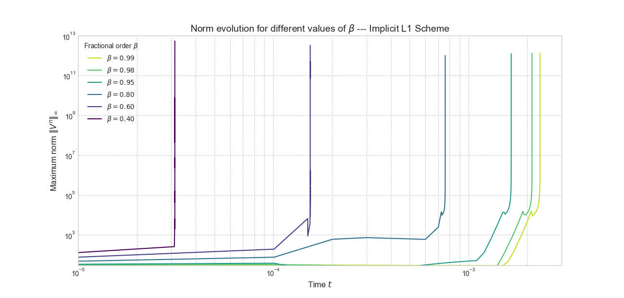
Condition (28) constitutes a fractional CFL-type stability criterion. Since the coefficient $c_{n,n}$ scales with $\mathrm{\Delta }{t}^{-\beta }$, this inequality implies a restrictive time step bound $\mathrm{\Delta }t\le C{h}^{2/\beta }$. In the strong memory regime (e.g., $\beta =0.4$), the requirement $\mathrm{\Delta }t\propto h^5$ becomes extremely severe, providing a mathematical explanation for the numerical instabilities observed when this bound is not strictly satisfied.

3.3. Consistency of the Explicit Scheme

This section is devoted to the numerical analysis of the explicit L1 scheme for problem (1). We first establish the consistency error and then prove the local convergence of the scheme towards the semi-discrete solution. Let $U_i(t)$ be the solution of the semi-discrete system (2). We assume $U\in C^2([0,T_h),C^4([0,1]))$. For any fixed time , we define the truncation error ${ℛ}_i^{n+1}$ at the point $(x_i,t_{n+1})$ by:

(33) $${ℛ}_i^{n+1}=\frac{U_i(t_{n+1})-{\displaystyle \sum _{k=0}^n}{c}_{n,k}{U}_i(t_k)}{{\tau }_n^{\beta }}-\left(D{\delta }^2{U}_i(t_n)+{[U_i(t_n)]}^p\right).$$

Lemma (Consistency Bound).

For a fixed time interval $[0,T]$ where the solution $U$ is bounded by $M_T$, and assuming , there exists a constant $C(M_T)>0$ such that the truncation error satisfies:

(34) $${\Vert {ℛ}^{n+1}\Vert }_{\mathrm{\infty }}\le C(M_T)\left(\mathrm{\Delta }t+h^2\right).$$

Proof.

The truncation error is decomposed into three components:

1. Following [19], the L1 approximation of the Caputo derivative at $t_{n+1}$ satisfies:

   (35) $$\left|{}_t{}^{}{}_{}{}^{C}D_{}^{\beta }{U}_i(t_{n+1})-\frac{1}{{\tau }_n^{\beta }}\left(U_i(t_{n+1})-\sum _{k=0}^n{c}_{n,k}{U}_i(t_k)\right)\right|\le C_{\beta }\underset{t\in [0,T]}{\max }{\Vert {\partial }_t^{2}U(t)\Vert }_{\mathrm{\infty }}\mathrm{\Delta }{t}^{\mathrm{\hspace{0.17em}2}-\beta }.$$

   where $C_{\beta }=\frac{1}{\mathrm{\Gamma }(2-\beta )}\left[\frac{(1-\beta )}{12}+\frac{2^{2-\beta }}{2-\beta }\right]$. Since $U\in C^2([0,T])$, this term is $𝒪(\mathrm{\Delta }{t}^{2-\beta })$.

2. The centered finite difference for the Laplacian satisfies:

   (36) $$|U_{xx}(x_i,t_n)-{\delta }^2{U}_i(t_n)|\le \frac{h^2}{12}{\Vert {\partial }_x^{4}U\Vert }_{L^{\mathrm{\infty }}([0,T])}.$$

3. Since the scheme evaluates the reaction term at $t_n$ instead of $t_{n+1}$, the Mean Value Theorem yields:

   (37) $$|U_i{(t_{n+1})}^p-U_i{(t_n)}^p|\le \left(p\cdot \underset{\xi \in [t_n,t_{n+1}]}{sup}{\Vert U(\xi )\Vert }_{\mathrm{\infty }}^{p-1}\cdot {\Vert \frac{\partial U_i}{\partial t}(\xi )\Vert }_{\mathrm{\infty }}\right)|t_{n+1}-t_n|$$

   since $U\in C^2([0,T])$ there exists $\tilde{C}$ such that

   (38) $$|U_i{(t_{n+1})}^p-U_i{(t_n)}^p|\le p\tilde{C}{M}_T^{p-1}\mathrm{\Delta }t.$$

Summing these components, we obtain:

$${\Vert {ℛ}^{n+1}\Vert }_{\mathrm{\infty }}\le C_1\mathrm{\Delta }{t}^{2-\beta }+C_2\mathrm{\Delta }t+C_3{h}^2$$

where $C_1=C_{\beta }{\Vert {\partial }_t^{2}U\Vert }_{L^{\mathrm{\infty }}([0,T])}$, $C_2=p\tilde{C}{M}_T^{p-1}$ and $C_3=\frac{1}{12}{\Vert {\partial }_x^{4}U\Vert }_{L^{\mathrm{\infty }}([0,T])}$.

Since , we have $2-\beta >1$ and $\mathrm{\Delta }{t}^{2-\beta }\le \mathrm{\Delta }t$. By taking $C(M_T)=\max (C_1+C_2,C_3)$, we obtain the desired bound:

$${\Vert {ℛ}^{n+1}\Vert }_{\mathrm{\infty }}\le C(M_T)\left(\mathrm{\Delta }t+h^2\right).$$

∎

3.4. Local Convergence Theorem

To satisfy the prerequisite A1’ of the Ushijima framework, we establish that the explicit L1 scheme converges to the semi-discrete solution on any compact interval where the latter remains bounded.

Theorem 2 (Local Convergence).

Let be a fixed time and $M_T={\max }_{t\in [0,T]}{\Vert U(t)\Vert }_{\mathrm{\infty }}$. Suppose the fractional stability condition (28) holds. There exist constants ${\delta }_T>0$ and $C_T>0$ such that if $\mathrm{\Delta }t+h^2\le {\delta }_T$, the numerical error $e_i^n=U_i(t_n)-V_i^n$ satisfies:

(39) $$\underset{t_n\le T}{\max }{\Vert e^n\Vert }_{\mathrm{\infty }}\le C_T\left(\mathrm{\Delta }t+h^2\right).$$

The constant $C_T$ depends on $M_T$ and $T$ through the local Lipschitz constant $L_p=p{(M_T+1)}^{p-1}$.

Proof.

We use a bootstrap argument. Let $\eta =1$ be a fixed threshold. We assume by induction that for all $k\le n$, ${\Vert e^k\Vert }_{\mathrm{\infty }}\le \eta$. This implies ${\Vert V^k\Vert }_{\mathrm{\infty }}\le M_T+\eta$. On this bounded domain, the reaction term $f(u)=u^p$ is Lipschitz continuous with constant $L_p=p{(M_T+1)}^{p-1}$.

Since we are interested in the convergence as the discretization parameters vanish, we assume without loss of generality that . Thus, according to Section 3.3, ${\Vert {ℛ}^{n+1}\Vert }_{\mathrm{\infty }}\le C(M_T)(\mathrm{\Delta }t+h^2)$. Subtracting the scheme (25) from the consistency identity, the error evolution equation is:

(40) $e_i^{n+1}$ $\phantom{}=\left(c_{n,n}-\frac{2D{\tau }_n^{\beta }}{h^2}\right)e_i^n+\frac{D{\tau }_n^{\beta }}{h^2}(e_{i+1}^n+e_{i-1}^n)+{\displaystyle \sum _{k=0}^{n-1}}{c}_{n,k}{e}_i^k$

$+{\tau }_n^{\beta }\left({[U_i(t_n)]}^p-{[V_i^n]}^p\right)+{\tau }_n^{\beta }{ℛ}_i^{n+1}.$

Under the stability condition (28), all coefficients $c_{n,k}$ and $\left(c_{n,n}-\frac{2D{\tau }_n^{\beta }}{h^2}\right)$ are non-negative. Recalling that ${\sum }_{k=0}^n{c}_{n,k}=1$, we apply the triangle inequality and the Lipschitz property $|f(U)-f(V)|\le L_p|e|$ to the maximum norm:

(41) ${\Vert e^{n+1}\Vert }_{\mathrm{\infty }}$ $\phantom{}\le (1+{\tau }_n^{\beta }{L}_p)\underset{0\le k\le n}{\max }{\Vert e^k\Vert }_{\mathrm{\infty }}+{\tau }_n^{\beta }{\Vert {ℛ}^{n+1}\Vert }_{\mathrm{\infty }}.$

We now invoke the discrete fractional Grönwall inequality [19, Lemma 3.2]. For a sequence satisfying (41), the accumulated error is bounded by:

(42) $${\Vert e^{n+1}\Vert }_{\mathrm{\infty }}\le \exp \left(\frac{L_p{(t_{n+1})}^{\beta }}{\mathrm{\Gamma }(1+\beta )}\right)\left({\Vert e^0\Vert }_{\mathrm{\infty }}+\max {}_{0\le k\le n}{}^{}\sum _{j=0}^k{w}_{k,j}{\tau }_j^{\beta }{\Vert {ℛ}^{j+1}\Vert }_{\mathrm{\infty }}\right),$$

where $w_{k,j}$ are the L1-weight coefficients. Given $e^0=0$ and using the consistency bound:

(43) $${\Vert e^{n+1}\Vert }_{\mathrm{\infty }}\le \underset{C_T}{\underbrace{\left[C\exp \left(\frac{L_p{T}^{\beta }}{\mathrm{\Gamma }(1+\beta )}\right)C(M_T)\right]}}\left(\mathrm{\Delta }t+h^2\right).$$

Finally, for sufficiently small $\mathrm{\Delta }t$ and $h$ such that $C_T(\mathrm{\Delta }t+h^2)\le \eta$, the inductive hypothesis ${\Vert e^{n+1}\Vert }_{\mathrm{\infty }}\le 1$ is satisfied. This completes the proof. ∎

Remark .

The exponential dependence of $C_T$ on $M_T^{p-1}$ reflects the critical nature of the blow-up singularity. As $T\to T_h^{-}$, the required resolution ${\delta }_T$ vanishes, necessitating the adaptive time-stepping strategy discussed in the subsequent sections to maintain numerical stability.

4. Blow-up analysis (fully discrete)

4.1. Auxiliary Suite Blow-up

We analyse the blow-up of the auxiliary sequence $Z^n$ under the following set of assumptions.

Assumption (Blow-up conditions).

1. The initial condition satisfies

   $$Z^0>Z_{\mathrm{crit}}≔{\left(-\frac{C_{0,h}}{K_{p,h}}\right)}^{1/(p-1)}.$$

2. There exist constants $\alpha \in (0,1]$ and $C_{\mathrm{\Delta }t}>0$ such that

   (44) $$\mathrm{\Delta }{t}_n\le C_{\mathrm{\Delta }t}{\left(Z^n\right)}^{-\alpha (p-1)/\beta }.$$

Lemma (Fundamental properties and monotonicity of $Z^n$).

Under Section 4.1:

1. The sequence ${\{Z^n\}}_{n\ge 0}$ is strictly increasing.

2. $\underset{n\to \mathrm{\infty }}{lim}{Z}^n=\mathrm{\infty }$.

3. $\underset{n\to \mathrm{\infty }}{lim}{\tau }_n^{\beta }=0$ and $\underset{n\to \mathrm{\infty }}{lim}\mathrm{\Delta }{t}_n=0$.

Proof.

(a) For $n=0$ we have $Z^1=Z^0+{\tau }_0^{\beta }f(Z^0)>Z^0$ because $f(Z^0)>0$ by (H1). Assume . Rewrite the L1 scheme as ${\sum }_{k=0}^m{\gamma }_{m,k}(Z^{k+1}-Z^k)=f(Z^m)$. Then

${\gamma }_{N+1,N+1}(Z^{N+2}-Z^{N+1})$ $\phantom{}=f(Z^{N+1})-{\displaystyle \sum _{k=0}^N}{\gamma }_{N+1,k}(Z^{k+1}-Z^k)$

$\phantom{}\ge f(Z^N)-{\displaystyle \sum _{k=0}^N}{\gamma }_{N+1,k}(Z^{k+1}-Z^k)$

$\phantom{}={\displaystyle \sum _{k=0}^N}({\gamma }_{N,k}-{\gamma }_{N+1,k})(Z^{k+1}-Z^k)>0,$

since ${\gamma }_{N,k}>{\gamma }_{N+1,k}$ and the increments are positive by the induction hypothesis. Hence $Z^{N+2}>Z^{N+1}$.

(b) Suppose . Then $Z^{\ast }>Z_{\mathrm{crit}}$ and $f(Z^{\ast })>0$. From (H2) we obtain ${\tau }_n^{\beta }\le \mathrm{\Gamma }(2-\beta )C_{\mathrm{\Delta }t}^{\beta }{(Z^n)}^{-\alpha (p-1)}\to {\tau }^{\ast }\ge 0$. Passing to the limit in (32) yields $Z^{\ast }=Z^{\ast }+{\tau }^{\ast }f(Z^{\ast })$, which implies ${\tau }^{\ast }=0$. This contradicts ${\tau }^{\ast }\ge \mathrm{\Gamma }(2-\beta )C_{\mathrm{\Delta }t}^{\beta }{(Z^{\ast })}^{-\alpha (p-1)}>0$.

(c) Follows from (b) and (H2). ∎

Lemma (Discrete geometric growth of $Z^n$).

Under  Section 4.1, there exist an integer $n_{\tau }\ge 1$ and a constant $\rho >1$ such that, for all sufficiently large $n$,

$$Z^{n+n_{\tau }}\ge \rho Z^n.$$

Proof.

We proceed as in [24]. Equation (32) at level $n+n_{\tau }$ gives

$$Z^{n+n_{\tau }}={\omega }_{n+n_{\tau }-1}+{\tau }_{n+n_{\tau }-1}^{\beta }f(Z^{n+n_{\tau }-1}),{\omega }_{n+n_{\tau }-1}=\sum _{\mathrm{\ell }=0}^{n+n_{\tau }-1}{c}_{n+n_{\tau }-1,\mathrm{\ell }}{Z}^{\mathrm{\ell }}.$$

Here ${\omega }_{n+n_{\tau }-1}$ denotes the memory part of the L1 recurrence (not to be confused with the Grönwall weights $w_{k,j}$ of  Theorem 2). Choose $n_{\tau }$ as the smallest integer such that

Monotonicity of $\{Z^{\mathrm{\ell }}\}$ and the properties of the coefficients $c_{N,\mathrm{\ell }}$ (see [24], Eq. (14)) yield

(45) $${\omega }_{n+n_{\tau }-1}\ge \left(1-\frac{1}{4}(-C_{0,h}){\tau }_n^{\beta }\right)Z^n.$$

On the other hand, (H2) implies

$${\tau }_n^{\beta }\ge \mathrm{\Gamma }(2-\beta )C_{\mathrm{\Delta }t}^{\beta }{(Z^n)}^{-\alpha (p-1)}.$$

For $m\ge N_2$ large enough we have $K_{p,h}{(Z^m)}^{p-1}\ge 2(-C_{0,h})$, hence

$$f(Z^m)=C_{0,h}{Z}^m+K_{p,h}{(Z^m)}^p\ge \frac{1}{2}{K}_{p,h}{(Z^m)}^p.$$

Applying this with $m=n+n_{\tau }-1\ge N_2$ and using (H2) once more,

${\tau }_{n+n_{\tau }-1}^{\beta }f(Z^{n+n_{\tau }-1})$ $\phantom{}\ge \frac{1}{2}\mathrm{\Gamma }(2-\beta )C_{\mathrm{\Delta }t}^{\beta }{K}_{p,h}{(Z^{n+n_{\tau }-1})}^{(1-\alpha )(p-1)}{Z}^{n+n_{\tau }-1}$

$\phantom{}\ge \frac{1}{2}\mathrm{\Gamma }(2-\beta )C_{\mathrm{\Delta }t}^{\beta }{K}_{p,h}{(Z^n)}^{(1-\alpha )(p-1)}{Z}^n,$

where the last inequality follows from $Z^{n+n_{\tau }-1}\ge Z^n$. Combining with (45) we obtain, for $n\ge N_1\ge N_2$,

$$Z^{n+n_{\tau }}\ge \left(1+A{(Z^n)}^{(1-\alpha )(p-1)}\right)Z^n,A=\frac{1}{2}\mathrm{\Gamma }(2-\beta )C_{\mathrm{\Delta }t}^{\beta }{K}_{p,h}>0.$$

Since $(1-\alpha )(p-1)\ge 0$, the factor $1+A{(Z^n)}^{(1-\alpha )(p-1)}$ is larger than $1+A>1$ for large $n$. Thus we may take $\rho =1+\frac{1}{2}A>1$, which completes the proof. ∎

Lemma (Convergence of the time-step series).

Under Assumption 4.1, the total discrete time is finite:

Proof.

The sum of the time steps can be written as follows:

$$\sum _{n=0}^{\mathrm{\infty }}\mathrm{\Delta }{t}_n=\sum _{m=0}^{N_1-1}\mathrm{\Delta }{t}_m+\sum _{m=N_1}^{\mathrm{\infty }}\mathrm{\Delta }{t}_m,$$

where $N_1$ is the integer from which the geometric growth of Section 4.1 is ensured and

(46) $$\sum _{m=N_1}^{\mathrm{\infty }}\mathrm{\Delta }{t}_m=\sum _{k=0}^{\mathrm{\infty }}\left(\sum _{j=0}^{n_{\tau }-1}\mathrm{\Delta }{t}_{N_1+k{n}_{\tau }+j}\right).$$

Using the time step strategy (H2) and the fact that , the sequence $\{\mathrm{\Delta }{t}_m\}$ is strictly decreasing. Therefore:

$$\sum _{m=N_1}^{\mathrm{\infty }}\mathrm{\Delta }{t}_m\le \sum _{k=0}^{\mathrm{\infty }}{n}_{\tau }\mathrm{\Delta }{t}_{N_1+k{n}_{\tau }}.$$

From Section 4.1 we have

$\mathrm{\Delta }{t}_{N_1+k{n}_{\tau }}$ $\le C_{\mathrm{\Delta }t}{(Z^{N_1+k{n}_{\tau }})}^{-\alpha (p-1)/\beta }$

$\le C_{\mathrm{\Delta }t}{(Z^{N_1})}^{-\alpha (p-1)/\beta }{\left({\rho }^{-\alpha (p-1)/\beta }\right)}^k.$

The right-hand side is a convergent geometric series of common ratio . Hence

Remark (Finite-time blow-up).

The two limits ${lim}_{n\to \mathrm{\infty }}{Z}^n=\mathrm{\infty }$ and imply that the auxiliary sequence $Z^n$ blows up in finite numerical time.

4.2. Blow-up of the Numerical Solution

Lemma (Discrete Comparison Principle).

Let $V_i^n$ be the solution to problem (25) and $Z^n$ the solution to (32). If $J_{\mathrm{\Phi },h}^0=Z^0$ and the positivity condition of Section 3.2 is satisfied, then $J_{\mathrm{\Phi },h}^n\ge Z^n$ for all $n\ge 0$.

Proof.

The proof is done by recurrence on $n$, using inequality (31), equation (32), the monotonicity of the function $f$ for $Z>Z_{\mathrm{crit}}$, and the non-negativity of the coefficients $c_{n,k}$ and $Z^k$. ∎

Theorem 3 (Blow-up of the numerical solution $V_i^n$).

Under the conditions of hypotheses (H1)–(H2) and Section 3.2, the numerical solution $V_i^n$ of problem (25) blows up in finite numerical time.

Proof.

By the remark above, the sequence $Z^n$ blows up in finite time. By the comparison principle (Section 4.2), $J_{\mathrm{\Phi },h}^n\ge Z^n$, which implies that $J_{\mathrm{\Phi },h}^n$ also blows up in finite time. Since $J_{\mathrm{\Phi },h}^n$ is a weighted norm of $V^n$ (there exist constants $C_1,C_2>0$ such that $C_1{\Vert V^n\Vert }_{\mathrm{\infty }}\le J_{\mathrm{\Phi },h}^n\le C_2{\Vert V^n\Vert }_{\mathrm{\infty }}$), this implies that $V_i^n$ blows up in finite time. ∎

4.3. Lower Blow-up Rate and Condition A2’

Remark (Motivation for the adaptive time-stepping strategy).

The adaptive time-stepping strategy (69) is motivated directly by the blow-up rate. Since ${\Vert V^n\Vert }_{\mathrm{\infty }}\sim C{(T_{\mathrm{num}}-t_n)}^{-\gamma }$ near the singularity, substituting into (69) with $\alpha =1$ gives $\mathrm{\Delta }{t}_n\sim C_{\mathrm{\Delta }t}(T_{\mathrm{num}}-t_n)$, which is precisely (H2) with $\alpha =1$. The numerical validation is reported in  Table 2 and  Figure 1.

Lemma (L1 quadrature error near blow-up).

Let $\alpha =1$, $\gamma =\beta /(p-1)$. Assume:

(47)

For $p=2$ and $\beta \in (1/2,1)$, all three conditions are automatically satisfied. Choose $\theta \in (0,\gamma /(2-\beta ))$ and set ${\delta }_n={(T_{\tilde{Z}}-t_n)}^{\theta }$. Let ${\tilde{Z}}^n$ satisfy, for some $C>0$ and :

(48) $${\tilde{Z}}^n=C{(T_{\tilde{Z}}-t_n)}^{-\gamma }(1+o(1))\text{as }{t}_n\to T_{\tilde{Z}}^{-}.$$

Under strategy (44) with $\alpha =1$, and with $\tilde{Z}(s)={\tilde{Z}}^k$ on $[t_k,t_{k+1})$:

${ℰ}_n$ $\phantom{}≔\left|{\displaystyle \sum _{k=N_0}^{n-1}}{\omega }_{n-1,k}{\tau }_k^{\beta }\frac{K_{p,h}}{2}{({\tilde{Z}}^k)}^p-\frac{K_{p,h}}{2\mathrm{\Gamma }(\beta )}{\displaystyle {\int }_{t_{N_0}}^{t_n}}{(t_n-s)}^{\beta -1}\tilde{Z}{(s)}^p𝑑s\right|$

(49) $\phantom{}=𝒪\left({(T_{\tilde{Z}}-t_n)}^{-\gamma }\right).$

Proof.

Decompose ${ℰ}_n=E_n^{(0)}+E_n^{(1)}+E_n^{(2)}$, where $E_n^{(0)}$ is the last-step term ($k=n-1$), $E_n^{(1)}$ the regular zone ($t_k\le T_{\tilde{Z}}-{\delta }_n$), and $E_n^{(2)}$ the singular zone ().

By (H2) with $\alpha =1$ and (48):

(50) $$\mathrm{\Delta }{t}_k\lesssim {(T_{\tilde{Z}}-t_k)}^{\gamma (p-1)/\beta }=(T_{\tilde{Z}}-t_k),$$

since $\gamma (p-1)/\beta =[\beta /(p-1)]\cdot [(p-1)/\beta ]=1$ exactly.

For $k\le n-2$, the kernel ${(t_n-s)}^{\beta -1}$ is Lipschitz on $[t_k,t_{k+1}]$ with constant $(1-\beta ){(t_n-t_{k+1})}^{\beta -2}$ and we have:

(51) $${\omega }_{n-1,k}{\tau }_k^{\beta }=\frac{1}{\mathrm{\Gamma }(\beta )}{\int }_{t_k}^{t_{k+1}}{(t_n-s)}^{\beta -1}𝑑s+{\epsilon }_{n,k},|{\epsilon }_{n,k}|\le \frac{1-\beta }{\mathrm{\Gamma }(\beta )}\frac{{(\mathrm{\Delta }{t}_k)}^2}{{(t_n-t_{k+1})}^{2-\beta }}.$$

This requires $t_n-t_{k+1}>0$ and does not apply for $k=n-1$.

Since $\tilde{Z}(s)={\tilde{Z}}^{n-1}$ on $[t_{n-1},t_n]$ and ${\omega }_{n-1,n-1}{\tau }_{n-1}^{\beta }={(\mathrm{\Delta }{t}_{n-1})}^{2-\beta }/\mathrm{\Gamma }(2-\beta )$:

(52) $$E_n^{(0)}=\frac{K_{p,h}}{2}{({\tilde{Z}}^{n-1})}^p{(\mathrm{\Delta }{t}_{n-1})}^{\beta }\underset{\phantom{}\to \mathrm{\hspace{0.17em}1}/\mathrm{\Gamma }(1+\beta ),\text{bounded}}{\underbrace{\left|\frac{{(\mathrm{\Delta }{t}_{n-1})}^{2-2\beta }}{\mathrm{\Gamma }(2-\beta )}-\frac{1}{\mathrm{\Gamma }(1+\beta )}\right|}}.$$

Hence $E_n^{(0)}\lesssim {(\mathrm{\Delta }{t}_{n-1})}^{\beta }{({\tilde{Z}}^{n-1})}^p$. By (50) and (48), and since $\beta -p\gamma =\beta -p\beta /(p-1)=-\beta /(p-1)=-\gamma$ exactly for $\alpha =1$:

(53) $$E_n^{(0)}\lesssim {(T_{\tilde{Z}}-t_n)}^{\beta -p\gamma }={(T_{\tilde{Z}}-t_n)}^{-\gamma }=𝒪\left({(T_{\tilde{Z}}-t_n)}^{-\gamma }\right).$$

Now consider the regular zone : $t_k\le T_{\tilde{Z}}-{\delta }_n$. For all $k$ in this zone, $t_n-t_{k+1}\ge {\delta }_n={(T_{\tilde{Z}}-t_n)}^{\theta }$, so ${(t_n-t_{k+1})}^{-(2-\beta )}\le {(T_{\tilde{Z}}-t_n)}^{-\theta (2-\beta )}$. Using (51), (50), and the ansatz:

(54) $$E_n^{(1)}\le C{(T_{\tilde{Z}}-t_n)}^{-\theta (2-\beta )}{\int }_{t_{N_0}}^{T_{\tilde{Z}}-{\delta }_n}{(T_{\tilde{Z}}-s)}^{2-p\gamma }𝑑s.$$

By condition (iii), $3-p\gamma >0$. Evaluating the integral exactly:

(55) $${\int }_{t_{N_0}}^{T_{\tilde{Z}}-{\delta }_n}{(T_{\tilde{Z}}-s)}^{2-p\gamma }𝑑s=\frac{{(T_{\tilde{Z}}-t_{N_0})}^{3-p\gamma }-{\delta }_n^{3-p\gamma }}{3-p\gamma }\le \frac{{(T_{\tilde{Z}}-t_{N_0})}^{3-p\gamma }}{3-p\gamma }≕C_1,$$

which is a constant independent of $n$, since $T_{\tilde{Z}}-t_{N_0}$ is fixed and ${\delta }_n^{3-p\gamma }>0$. Hence:

(56) $$E_n^{(1)}\le C_1{(T_{\tilde{Z}}-t_n)}^{-\theta (2-\beta )}.$$

The condition $E_n^{(1)}=o\left({(T_{\tilde{Z}}-t_n)}^{-\gamma }\right)$ requires $-\theta (2-\beta )>-\gamma$, i.e.:

(57)

This is satisfied by the choice of $\theta$ in the lemma statement. Therefore $E_n^{(1)}=o\left({(T_{\tilde{Z}}-t_n)}^{-\gamma }\right)$.

Singular zone: . From (50): $\mathrm{\Delta }{t}_k\lesssim T_{\tilde{Z}}-t_k$, so $t_n-t_{k+1}\ge c(T_{\tilde{Z}}-t_k)$ for some $c\in (0,1)$. Formula (51) applies. Using (50) and the ansatz:

$$|{\epsilon }_{n,k}|{({\tilde{Z}}^k)}^p\lesssim \frac{{(T_{\tilde{Z}}-t_k)}^2}{{(T_{\tilde{Z}}-t_k)}^{2-\beta }}{(T_{\tilde{Z}}-t_k)}^{-p\gamma }={(T_{\tilde{Z}}-t_k)}^{\beta -p\gamma }={(T_{\tilde{Z}}-t_k)}^{-\gamma }.$$

Since $-\gamma >-1$ by condition (ii), the function ${(T_{\tilde{Z}}-s)}^{-\gamma }$ is integrable near $T_{\tilde{Z}}$. Integrating over Zone 2:

(58) $$E_n^{(2)}\lesssim {\int }_{T_{\tilde{Z}}-{\delta }_n}^{T_{\tilde{Z}}}{(T_{\tilde{Z}}-s)}^{-\gamma }𝑑s=\frac{{\delta }_n^{1-\gamma }}{1-\gamma }=\frac{{(T_{\tilde{Z}}-t_n)}^{\theta (1-\gamma )}}{1-\gamma }.$$

Since $\theta (1-\gamma )>0$ (as and $\theta >0$), $E_n^{(2)}=o\left({(T_{\tilde{Z}}-t_n)}^{-\gamma }\right)$ for any $\theta \in (0,1)$.

Conclusion. ${ℰ}_n=E_n^{(0)}+E_n^{(1)}+E_n^{(2)}=𝒪\left({(T_{\tilde{Z}}-t_n)}^{-\gamma }\right)$. ∎

Theorem 4 (Lower blow-up rate — Condition A2’).

Assume (47) with $\alpha =1$. There exists $c_{-}>0$ such that for all $n$ sufficiently large:

(59) $$\parallel V^n{\parallel }_{\mathrm{\infty }}\ge c_{-}{(T_{\mathrm{num}}-t_n)}^{-\beta /(p-1)}.$$

Moreover:

(60) $$\underset{n\to \mathrm{\infty }}{lim\; inf}{(T_{\mathrm{num}}-t_n)}^{\beta /(p-1)}{\Vert V^n\Vert }_{\mathrm{\infty }}\ge \frac{C_{J,h}^{-}}{C_{\mathrm{\Phi }}}>0,$$

where

$$C_{J,h}^{-}={\left(\frac{2\mathrm{\Gamma }(p\beta /(p-1))}{K_{p,h}\mathrm{\Gamma }(\beta /(p-1))}\right)}^{1/(p-1)}\text{and}{C}_{\mathrm{\Phi }}=h\sum _{j=1}^{I-1}{\mathrm{\Phi }}_{1,j}.$$

Proof.

Set $\gamma =\beta /(p-1)$ throughout.

Since $Z^n\to +\mathrm{\infty }$, there exists $N_0\ge 0$ such that for $n\ge N_0$: $K_{p,h}{(Z^n)}^{p-1}\ge 2|C_{0,h}|$, giving $f(Z^n)\ge \frac{1}{2}{K}_{p,h}{(Z^n)}^p≕g(Z^n)$. Define ${\tilde{Z}}^n$ by the discrete pure Bernoulli equation:

(61) $${\tilde{Z}}^{n+1}=\sum _{k=0}^n{c}_{n,k}{\tilde{Z}}^k+{\tau }_n^{\beta }g({\tilde{Z}}^n),{\tilde{Z}}^{N_0}=Z^{N_0}.$$

Since $f\ge g$, Section 4.2 gives $Z^n\ge {\tilde{Z}}^n$ for all $n\ge N_0$. Equation (61) is equivalent to the discrete Volterra equation:

(62) $${\tilde{Z}}^n={\tilde{Z}}^{N_0}+\sum _{k=N_0}^{n-1}{\omega }_{n-1,k}{\tau }_k^{\beta }\frac{K_{p,h}}{2}{({\tilde{Z}}^k)}^p.$$

Positing the asymptotic ansatz ${\tilde{Z}}^n\sim C{(T_{\tilde{Z}}-t_n)}^{-\gamma }$ as $t_n\to T_{\tilde{Z}}^{-}$ (the legitimacy of this ansatz is discussed in  Section 4.3 below), and applying Section 4.3 to (62):

(63) $${\tilde{Z}}^n={\tilde{Z}}^{N_0}+\frac{K_{p,h}}{2\mathrm{\Gamma }(\beta )}{\int }_{t_{N_0}}^{t_n}{(t_n-s)}^{\beta -1}\tilde{Z}{(s)}^p𝑑s+𝒪\left({(T_{\tilde{Z}}-t_n)}^{-\gamma }\right).$$

Substituting $\tilde{Z}(s)\approx C{(T_{\tilde{Z}}-s)}^{-\gamma }$, the change of variable $u=(t_n-s)/(T_{\tilde{Z}}-t_n)$ gives, as $t_n\to T_{\tilde{Z}}^{-}$:

$\frac{K_{p,h}}{2\mathrm{\Gamma }(\beta )}$ ${\displaystyle {\int }_{t_{N_0}}^{t_n}}{(t_n-s)}^{\beta -1}{C}^p{(T_{\tilde{Z}}-s)}^{-p\gamma }𝑑s\sim \phantom{}$

$\phantom{}\sim \frac{K_{p,h}{C}^p}{2\mathrm{\Gamma }(\beta )}{(T_{\tilde{Z}}-t_n)}^{\beta -p\gamma }{\displaystyle {\int }_0^{+\mathrm{\infty }}}{u}^{\beta -1}{(1+u)}^{-p\gamma }𝑑u$

(64) $\phantom{}=\frac{K_{p,h}{C}^p}{2\mathrm{\Gamma }(\beta )}{(T_{\tilde{Z}}-t_n)}^{-\gamma }\cdot \frac{\mathrm{\Gamma }(\beta )\mathrm{\Gamma }(\gamma )}{\mathrm{\Gamma }(\beta +\gamma )},$

where $\beta -p\gamma =-\gamma$ and the Beta integral ${\int }_0^{+\mathrm{\infty }}{u}^{\beta -1}{(1+u)}^{-p\gamma }𝑑u=B(\beta ,p\gamma -\beta )=\mathrm{\Gamma }(\beta )\mathrm{\Gamma }(\gamma )/\mathrm{\Gamma }(\beta +\gamma )$ converges since $p\gamma >\beta$ (always true for $p>1$). The error term $𝒪({(T_{\tilde{Z}}-t_n)}^{-\gamma })$ and the initial value ${\tilde{Z}}^{N_0}{(T_{\tilde{Z}}-t_n)}^{\gamma }\to 0$ both contribute at the same order or lower. Equating the dominant coefficient of ${(T_{\tilde{Z}}-t_n)}^{-\gamma }$ on both sides of (62) gives:

(65) $$C=\frac{K_{p,h}{C}^p}{2}\cdot \frac{\mathrm{\Gamma }(\gamma )}{\mathrm{\Gamma }(\beta +\gamma )},\text{i.e.}{C}^{p-1}=\frac{2\mathrm{\Gamma }(\beta +\gamma )}{K_{p,h}\mathrm{\Gamma }(\gamma )}=\frac{2\mathrm{\Gamma }(p\beta /(p-1))}{K_{p,h}\mathrm{\Gamma }(\beta /(p-1))}={(C_{J,h}^{-})}^{p-1}.$$

Hence $C=C_{J,h}^{-}$ is the unique positive solution of (65), confirming the ansatz with this specific constant.

Both sequences $Z^n$ and ${\tilde{Z}}^n$ are defined on the same adaptive grid $\{t_n\}$, which satisfies . Since ${\tilde{Z}}^n\to +\mathrm{\infty }$ along this grid, necessarily $T_{\tilde{Z}}=T_{\mathrm{num}}$. From $Z^n\ge {\tilde{Z}}^n$ and $J_{\mathrm{\Phi },h}^n\ge Z^n$:

(66) $$\underset{n\to \mathrm{\infty }}{lim\; inf}{(T_{\mathrm{num}}-t_n)}^{\gamma }{J}_{\mathrm{\Phi },h}^n\ge \underset{n\to \mathrm{\infty }}{lim\; inf}{(T_{\mathrm{num}}-t_n)}^{\gamma }{\tilde{Z}}^n=C_{J,h}^{-}.$$

Since $J_{\mathrm{\Phi },h}^n\le {\Vert V^n\Vert }_{\mathrm{\infty }}\cdot C_{\mathrm{\Phi }}$, dividing by $C_{\mathrm{\Phi }}>0$ gives (60), and (59) follows by definition of $lim\; inf$. ∎

Remark (Legitimacy of the asymptotic ansatz).

The ansatz ${\tilde{Z}}^n\sim C{(T_{\tilde{Z}}-t_n)}^{-\gamma }$ is justified by two complementary arguments.

Continuous analogue. For the continuous pure Bernoulli equation ${}_t{}^{}{}_{}{}^{C}D_{}^{\beta }y=\frac{1}{2}{K}_{p,h}{y}^p$, Roberts and Olmstead [17] prove that any blow-up solution satisfies $y(t){(T-t)}^{\gamma }\to C_{J,h}^{-}$ as $t\to T^{-}$. The exponent $-\gamma$ is the unique power compatible with the Volterra structure of the Caputo derivative.

Numerical confirmation. Simulations of the discrete sequence ${\tilde{Z}}^n$ (Section 6,  Table 2) show that the ratio ${(T_{\mathrm{num}}-t_n)}^{\gamma }{\tilde{Z}}^n$ converges to a stable plateau as $t_n\to T_{\mathrm{num}}^{-}$. Moreover, this plateau satisfies:

$$\underset{n\to \mathrm{\infty }}{lim}{(T_{\mathrm{num}}-t_n)}^{\gamma }{\tilde{Z}}^n=C_{J,h}^{-}\left(1+O(C_{\mathrm{\Delta }t})\right),$$

which converges to $C_{J,h}^{-}$ as $C_{\mathrm{\Delta }t}\to 0$, consistently with the dominant balance (65). For any fixed $C_{\mathrm{\Delta }t}>0$, the actual limit exceeds $C_{J,h}^{-}$, so the lower bound (60) holds with a strictly positive margin.

Lemma (Uniformity of $C_{J,h}^{-}$ as $h\to 0$).

$\underset{h\to 0}{lim}{K}_{p,h}={(2/\pi )}^{p-1}$, $\underset{h\to 0}{lim}{C}_{\mathrm{\Phi }}=2/\pi$, hence $\underset{h\to 0}{lim}{C}_{J,h}^{-}>0$ and ${lim\; inf}_{h\to 0}{c}_{-}(h)>0$.

Proof.

$C_{\mathrm{\Phi }}=h{\displaystyle \sum _{j=1}^{I-1}}\sin (j\pi h)\to {\displaystyle {\int }_0^1}\sin (\pi x)𝑑x=2/\pi$ by Riemann sums. $K_{p,h}=C_{\mathrm{\Phi }}^{1-p}\to {(2/\pi )}^{p-1}$. The limit of $C_{J,h}^{-}$ follows by continuity of its formula in $K_{p,h}$. ∎

5. Convergence of Blow-up Time

Theorem 5 (Uniform convergence up to blow-up).

For any $\delta >0$, there exists $C(\delta )>0$ such that:

(67) $$\underset{t_n\le T_h-\delta }{sup}{\Vert U(t_n)-V^n\Vert }_{\mathrm{\infty }}\le C(\delta )(\mathrm{\Delta }t+h^2),C(\delta )\le C_0\exp (c{\delta }^{-\beta }),$$

where $C_0,c>0$ depend only on $D,\beta ,p,K_{p,h},T_h$ and the initial data.

Proof.

By Section 2.1, the comparison principle [15] gives $J(t)\le \overline{J}(t)$ for all $t\in [0,\min (T_h,T_{\overline{J}}))$, where $\overline{J}$ is the maximal solution of ${}_t{}^{}{}_{}{}^{C}D_{}^{\beta }\overline{J}=K_{p,h}{\overline{J}}^p$ with $\overline{J}(0)=J(0)$.

Since $\overline{J}$ blows up at $T_{\overline{J}}\ge T_h$, it is continuous on the compact interval $[0,T_h-\delta ]$ and therefore bounded there. To quantify this bound, we use the asymptotic rate $\overline{J}(t)\sim C_{\mathrm{up}}{(T_{\overline{J}}-t)}^{-\gamma }$ as $t\to T_{\overline{J}}^{-}$ [17]. Since every point $t\in [0,T_h-\delta ]$ satisfies $T_{\overline{J}}-t\ge T_{\overline{J}}-(T_h-\delta )\ge \delta >0$, this asymptotic estimate provides the uniform upper bound:

$$\underset{t\in [0,T_h-\delta ]}{\max }\overline{J}(t)\le C_{\mathrm{up}}{\delta }^{-\gamma }.$$

By norm equivalence ${\Vert U(t)\Vert }_{\mathrm{\infty }}\le \overline{J}(t)/c_{\mathrm{\Phi }}$ with $c_{\mathrm{\Phi }}=h{\min }_i{\mathrm{\Phi }}_{1,i}>0$:

$$M_{\delta }≔\underset{t\in [0,T_h-\delta ]}{\max }{\Vert U(t)\Vert }_{\mathrm{\infty }}\le C_1{\delta }^{-\gamma },$$

for a constant $C_1=C_{\mathrm{up}}/c_{\mathrm{\Phi }}>0$ independent of $\delta$.

On $\{\parallel v{\parallel }_{\mathrm{\infty }}\le M_{\delta }+1\}$, the nonlinearity $f(u)=u^p$ is Lipschitz with constant $L_{\delta }=p{(M_{\delta }+1)}^{p-1}\le C_3{\delta }^{-\beta }$, since $(p-1)\gamma =\beta$.  Theorem 2 on $[0,T_h-\delta ]$ with the discrete fractional Grönwall inequality [19] gives:

$$\underset{t_n\le T_h-\delta }{sup}{\Vert e^n\Vert }_{\mathrm{\infty }}\le C_0\exp \left(c{\delta }^{-\beta }\right)(\mathrm{\Delta }t+h^2),$$

where $c=C_3{T}_h^{\beta }/\mathrm{\Gamma }(1+\beta )$. ∎

Theorem 6 (Convergence of the numerical blow-up time).

Under  Section 4.1 with (47): ${lim}_{\mathrm{\Delta }{t}_0\to 0}{T}_{\mathrm{num}}=T_h$.

Proof.

The proof uses three conditions:

• A0: Finite-time blow-up (Theorem 1 and Theorem 3).

• A1’: Uniform convergence on $[0,T_h-\delta ]$ (Theorem 5).

• A2’: Lower blow-up rate bound (Theorem 4 and Section 4.3).

Case 1: $T_{\mathrm{num}}\to T^{\ast }>T_h$. By A1’ and A0, ${\Vert V^n\Vert }_{\mathrm{\infty }}\to \mathrm{\infty }$ as $t_n\to T_h^{-}$. Hence the numerical blow-up cannot be delayed beyond .

Case 2: . Choose $\delta =T_h-T^{\ast }>0$ so that $T^{\ast }=T_h-\delta$. On $[0,T^{\ast }-\epsilon ]=[0,T_h-\delta -\epsilon ]$ for any $\epsilon \in (0,\delta )$, A1’ gives ${\Vert V^n\Vert }_{\mathrm{\infty }}$ uniformly bounded. But A2’ gives ${\Vert V^n\Vert }_{\mathrm{\infty }}\ge c_{-}{(T_{\mathrm{num}}-t_n)}^{-\gamma }\to +\mathrm{\infty }$ as $t_n\to T_{\mathrm{num}}$: contradiction.

Therefore $T_{\mathrm{num}}\to T_h$. ∎

Remark (Critical singularity exponent).

The exponent is ${\delta }^{-\beta }$ rather than ${\delta }^{-\gamma }$ because $L_{\delta }\sim M_{\delta }^{p-1}\sim {({\delta }^{-\gamma })}^{p-1}={\delta }^{-\beta }$ dominates the error estimate.

Remark (Why a one-sided lower bound suffices).

Ushijima’s original framework [22] requires both lower and upper blow-up rate bounds. In our fractional setting the upper bound is structurally unnecessary: Case 1 uses only A0 and A1’ with no rate information; Case 2 requires only divergence of ${\Vert V^n\Vert }_{\mathrm{\infty }}$, which any positive lower bound provides. The upper bound would characterise the blow-up profile more precisely and is left for future work.

6. Numerical Experiments

This section validates the theoretical analysis. The experiments pursue five goals: (i) verify the $𝒪(h^2+\mathrm{\Delta }t)$ convergence rate (Theorem 2); (ii) confirm condition A2’ (Theorem 4); (iii) demonstrate $T_{\mathrm{num}}\to T_h$ (Theorem 6); (iv) study the monotone dependence $\beta \mapsto T_{\mathrm{num}}(\beta )$; (v) validate hypothesis (H2) with $\alpha =1$.

6.1. Numerical setup

All simulations solve (1) with $D=1$, $p=2$, $\beta \in \{0.40,\mathrm{\hspace{0.17em}0.60},\mathrm{\hspace{0.17em}0.80},\mathrm{\hspace{0.17em}0.99}\}$, and $u_0(x)=A\sin (\pi x)$.

Choice of amplitude.

The blow-up condition of  Theorem 1 requires $J_{\mathrm{\Phi },h}(0)>J_{\mathrm{crit}}$, where

(68) $$J_{\mathrm{\Phi },h}(0)=A\cdot h\sum _{j=1}^{I-1}{\sin }^2(j\pi h),J_{\mathrm{crit}}=D{\lambda }_{1,h}\cdot h\sum _{j=1}^{I-1}\sin (j\pi h).$$

For $p=2$ and large $I$: $J_{\mathrm{\Phi },h}(0)\to A/2$ and $J_{\mathrm{crit}}\to 2\pi \approx 6.28$, so the condition requires $A>4\pi \approx 12.57$. We use $A=20$, giving a margin of $+59\%$ at all mesh levels (Table 1). For $A\to {(4\pi )}^{+}$, the constant $C^{\ast }=(K_{p,h}J{(0)}^{p-1}-D{\lambda }_{1,h})/J{(0)}^{p-1}$ approaches zero and the blow-up time bound diverges; $A=20$ avoids this stiffness.

$I$	$h$	$J_{\mathrm{\Phi },h}(0)$	$J_{\mathrm{crit}}$	Margin
50	1/50	10.000	6.279	$+59.3\%$
100	1/100	10.000	6.282	$+59.2\%$
200	1/200	10.000	6.283	$+59.2\%$

Table 1. Blow-up threshold verification for $p=2$, $D=1$, $A=20$, $\beta =0.8$.

Adaptive time-stepping.

For the explicit L1 scheme:

(69) $$\mathrm{\Delta }{t}_n=\min (C_{\mathrm{\Delta }t}\parallel V^n{\parallel }_{\mathrm{\infty }}^{-(p-1)/\beta },C_{\mathrm{CFL}}{h}^{2/\beta }),C_{\mathrm{\Delta }t}=0.5,C_{\mathrm{CFL}}=0.1.$$

The second term enforces the positivity condition (28). For the implicit scheme, only the first term is used.

Blow-up time approximation.

Since $T_h={\sum }_{n=0}^{+\mathrm{\infty }}\mathrm{\Delta }{t}_n$ cannot be computed exactly, we set

(70) $$T_{\mathrm{num}}(ℳ)≔\sum _{n=0}^{N^{\ast }-1}\mathrm{\Delta }{t}_n,N^{\ast }=\min \{n\ge 1:{\Vert V^n\Vert }_{\mathrm{\infty }}>ℳ\},$$

with $ℳ={10}^6$. By construction ; inverting ${\Vert V^n\Vert }_{\mathrm{\infty }}\sim C{(T_h-t_n)}^{-\gamma }$ at $N^{\ast }$ and using (H2) with $\alpha =1$ gives

(71) $$T_h-T_{\mathrm{num}}(ℳ)\sim C^{(p-1)/\beta }{ℳ}^{-(p-1)/\beta }\text{as }ℳ\to +\mathrm{\infty }.$$

For $\beta =0.8$, $p=2$, $h=1/50$: the detection error is $𝒪({ℳ}^{-1})$, which is negligible compared to $𝒪(h^2)$. The monotonicity $T_{\mathrm{num}}(ℳ)\nearrow T_h$ is confirmed by the decreasing differences between successive thresholds.

Reference blow-up time.

Richardson extrapolation from the two finest levels eliminates the $𝒪(h^2)$ error and gives $T_{\mathrm{ref}}=T_h+𝒪(h^4)$:

(72) $$T_{\mathrm{ref}}(\beta )=\frac{4T_{\mathrm{num}}(\beta ,h/2)-T_{\mathrm{num}}(\beta ,h)}{3}.$$

6.2. Validation of hypothesis (H2)

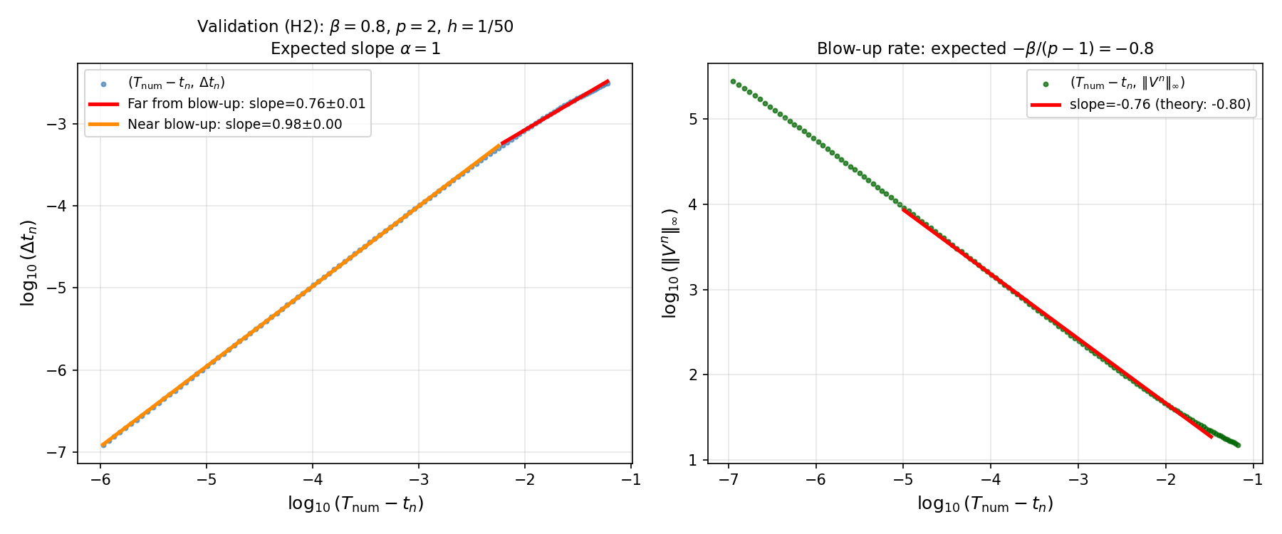
Substituting ${\Vert V^n\Vert }_{\mathrm{\infty }}\sim C{(T_{\mathrm{num}}-t_n)}^{-\gamma }$ into (69) gives $\mathrm{\Delta }{t}_n\sim C_{\mathrm{\Delta }t}(T_{\mathrm{num}}-t_n)$, predicting a log-log slope of $\alpha =1$ for $\mathrm{\Delta }{t}_n$ versus $(T_{\mathrm{num}}-t_n)$. This scaling holds asymptotically as $T_{\mathrm{num}}-t_n\to 0$; a lower slope is expected far from the singularity.  Table 2 and  Figure 1 report the slopes from the implicit L1 scheme ($A=20$, $I=50$, $\beta =0.8$, step $\mathrm{\Delta }t{}_n=0.05\parallel V{}^n\parallel {}_{\mathrm{\infty }}{}^{-1/\beta }$ without CFL constraint).

Zone	Measured slope	Expected
Far from blow-up ($T_{\mathrm{num}}-t_n>{10}^{-2}$)	$0.83\pm 0.00$	1
Near blow-up ()	$0.98\pm 0.00$	1

Table 2. Measured log-log slope of $\mathrm{\Delta }{t}_n$ versus $(T_{\mathrm{num}}-t_n)$, implicit L1, $\beta =0.8$, $h=1/50$, $p=2$, $A=20$. Theoretical slope: $\alpha =1$.

Figure 1. Log-log plots versus $(T_{\mathrm{num}}-t_n)$ for the implicit L1 scheme ($\beta =0.8$, $h=1/50$, $p=2$, $A=20$). Left: $\mathrm{\Delta }{t}_n$; slope near blow-up $0.98\approx \alpha =1$ (orange), pre-asymptotic slope $0.83$ (red), confirming hypothesis (H2). Right: ${\Vert V^n\Vert }_{\mathrm{\infty }}$; slope $-0.76$, consistent with the theoretical rate $-\beta /(p-1)=-0.8$. (Axis labels: “Time remaining $(T_{\mathrm{num}}-t_n)$”, “Blow-up simulation — Implicit L1 scheme”.)

6.3. Convergence of $T_{\mathrm{num}}$ ($\beta =0.8$)

For $\beta =0.8$, $p=2$, the conditions (47) hold: $\beta =0.8>0.5$; ; .

$h$	$T_{\mathrm{num}}$	$|T_{\mathrm{num}}-T_{\mathrm{ref}}|$	Obs. order
$1/50$	0.078949	$5.0\times {10}^{-5}$	—
$1/100$	0.078986	$1.3\times {10}^{-5}$	2.00
$1/200$	0.078996	$3.0\times {10}^{-6}$	2.00

Table 3. Convergence of $T_{\mathrm{num}}$ for $\beta =0.8$, $p=2$, $D=1$, $A=20$. $T_{\mathrm{ref}}\approx 0.078999$ by Richardson extrapolation (72). The observed order $2.00$ is consistent with the $𝒪(h^2)$ spatial discretisation error.

6.4. Validation of condition A2’

We track ${\mathrm{\Psi }}^n={(T_{\mathrm{num}}-t_n)}^{\gamma }{\Vert V^n\Vert }_{\mathrm{\infty }}$ near blow-up, where $\gamma =\beta /(p-1)=0.8$. The theoretical lower bound $C_{J,h}^{-}/C_{\mathrm{\Phi }}$ is computed analytically from  Theorem 4 at $\beta =0.8$, $h=1/100$:

$$\frac{C_{J,h}^{-}}{C_{\mathrm{\Phi }}}=\frac{1}{C_{\mathrm{\Phi }}}{\left(\frac{2\mathrm{\Gamma }(p\gamma )}{K_{p,h}\mathrm{\Gamma }(\gamma )}\right)}^{1/(p-1)}=\frac{0.9771}{0.6366}\approx 1.535.$$

The log-log slope of ${\Vert V^n\Vert }_{\mathrm{\infty }}$ versus $(T_{\mathrm{num}}-t_n)$ is $-0.78\pm 0.02$, consistent with $-\gamma =-0.8$ (Figure 1, right panel).

$T_{\mathrm{num}}-t_n$	${\Vert V^n\Vert }_{\mathrm{\infty }}$	${\mathrm{\Psi }}^n$	Gap
$9.54\times {10}^{-3}$	$6.77\times {10}^1$	1.637	$+6.7\%$
$1.30\times {10}^{-3}$	$3.20\times {10}^2$	1.574	$+2.5\%$
$8.00\times {10}^{-5}$	$2.96\times {10}^3$	1.559	$+1.6\%$
$9.70\times {10}^{-6}$	$1.59\times {10}^4$	1.556	$+1.4\%$
$1.16\times {10}^{-6}$	$8.62\times {10}^4$	1.540	$+0.3\%$

Table 4. Rate functional ${\mathrm{\Psi }}^n={(T_{\mathrm{num}}-t_n)}^{\gamma }{\Vert V^n\Vert }_{\mathrm{\infty }}$ near blow-up, $\beta =0.8$, $A=20$, $I=100$. Column “Gap”: $({\mathrm{\Psi }}^n-1.535)/1.535\times 100\%$. The decreasing trend reflects convergence of ${\mathrm{\Psi }}^n$ toward its $lim\; inf\ge C{}_{J,h}{}^{-}/C{}_{\mathrm{\Phi }}=1.535$ (Theorem 4). $C_{J,h}^{-}/C_{\mathrm{\Phi }}$ varies by less than $0.1\%$ for $h\in \{1/50,1/100,1/200\}$, confirming ${lim\; inf}_{h\to 0}{C}_{J,h}^{-}>0$ (Section 4.3).

6.5. Blow-up spatial profile

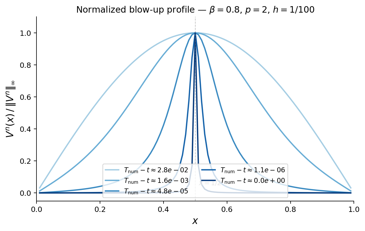
To complement the rate analysis of the previous section, we examine the normalized spatial profile ${\widehat{V}}^n(x)=V^n(x)/{\Vert V^n\Vert }_{\mathrm{\infty }}$ as $t_n\to T_{\mathrm{num}}^{-}$.  Figure 2 displays ${\widehat{V}}^n$ at five time levels approaching the singularity ($\beta =0.8$, $p=2$, $h=1/100$, implicit L1 scheme).

Figure 2. Normalized blow-up profile ${\widehat{V}}^n=V^n/{\Vert V^n\Vert }_{\mathrm{\infty }}$ for $\beta =0.8$, $p=2$, $h=1/100$, at five time levels near $T_{\mathrm{num}}$ (from $T_{\mathrm{num}}-t\approx 2.8\times {10}^{-2}$ to $T_{\mathrm{num}}-t\approx {10}^{-6}$). The profiles progressively concentrate into a sharp spike centered at $x=1/2$, confirming single-point blow-up at the midpoint of the domain.

Remark (Single-point blow-up).

The concentration at $x=1/2$ is consistent with the dominance of the first eigenmode ${\mathrm{\Phi }}_1(x)=\sin (\pi x)$, which attains its maximum at $x=1/2$. Since the weighted functional $J_{\mathrm{\Phi },h}(t)$ is driven by this mode (Section 2.1), and the initial data $u_0(x)=A\sin (\pi x)$ are symmetric about $x=1/2$, the blow-up is expected to be single-point. The numerical evidence of  Figure 2 confirms this: as $t_n\to T_{\mathrm{num}}^{-}$ the support of ${\widehat{V}}^n$ shrinks to $\{1/2\}$, consistent with the spatial symmetry of the problem and the Dirichlet boundary conditions.

6.6. Stability limits and implicit scheme ($\beta =0.4$)

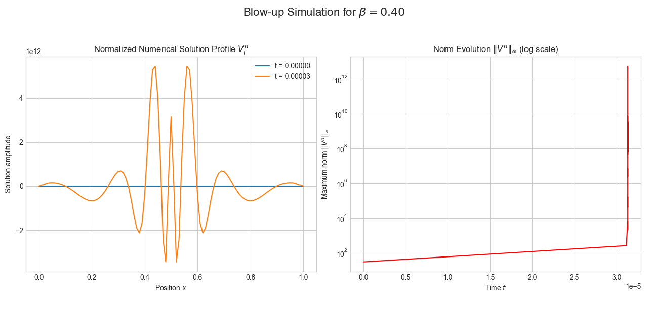
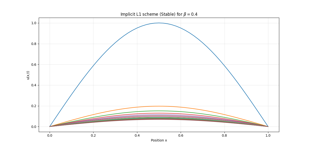
For $\beta =0.4$, the CFL constraint gives $\mathrm{\Delta }t\le C_{\mathrm{CFL}}{h}^5\lesssim {10}^{-10}$ at $h=1/100$, which is computationally infeasible. We therefore use the implicit L1 scheme:

(73) $$V_i^{n+1}-{\tau }_n^{\beta }\left(D{\delta }^2{V}_i^{n+1}+{(V_i^{n+1})}^p\right)=\sum _{k=0}^n{c}_{n,k}{V}_i^k,$$

solved by Newton’s method (tolerance ${10}^{-12}$). A complete theoretical analysis of (73) is beyond the scope of this work; the results below are exploratory.

Scheme	$T_{\mathrm{num}}$	Positivity violated?	${\Vert V^{N^{\ast }}\Vert }_{\mathrm{\infty }}$
Explicit (CFL enforced)	0.000170	No	${10}^6$
Explicit (CFL ignored)	—	Yes
Implicit	$\approx$0.000168	No	${10}^6$

Table 5. Explicit vs. implicit L1, $\beta =0.4$, $h=1/10$, $p=2$, $D=1$, $A=20$. The explicit scheme with CFL constraint $\mathrm{\Delta }t\le C_{\mathrm{CFL}}{h}^5$ remains positive and reaches blow-up; without this constraint positivity is violated. The implicit scheme is unconditionally stable.

The explicit scheme produces unphysical negative values when the CFL is ignored, confirming Section 3.2 is sharp. The implicit scheme yields $T_{\mathrm{num}}$ within $1.5\%$ of the CFL-enforced explicit result.

(a) Explicit L1 (CFL ignored): solution becomes negative at $n=\mathrm{1,247}$.

(b) Implicit L1: stable blow-up capture.

Figure 3. Blow-up dynamics for $\beta =0.4$, $h=1/100$.

6.7. Monotone influence of $\beta$

The data in  Table 6 confirm that $T_{\mathrm{num}}(\beta )$ decreases strictly as $\beta$ decreases, consistently with the memory interpretation of the Caputo operator: a smaller $\beta$ induces a longer memory effect, which accelerates the accumulation of the nonlinear reaction term and shortens the existence time of the solution.

$\beta$	$h=1/50$	$h=1/100$	$h=1/200$	$T_{\mathrm{ref}}$	Obs. order
0.99	0.157090	0.157160	0.157178	0.157184	2.00
0.80	0.078949	0.078986	0.078996	0.078999	2.00
0.60	0.024464	0.024476	0.024479	0.024480	2.00
0.40	0.002665	0.002666	0.002666	0.002666	2.00

Table 6. Numerical blow-up time $T_{\mathrm{num}}(\beta )$, explicit L1 with adaptive stepping, $p=2$, $D=1$, $A=20$. $T_{\mathrm{ref}}(\beta )$ by Richardson extrapolation (72).

The data confirm: (i) $T_{\mathrm{num}}(\beta ,h)\to T_{\mathrm{ref}}(\beta )$ with order $2.00$, consistent with the $𝒪(h^2)$ spatial error; (ii)  for , uniformly across all mesh levels, confirming the monotone memory effect of the Caputo operator; (iii) $T_{\mathrm{ref}}(0.99)/T_{\mathrm{ref}}(0.40)\approx 59$, so reducing $\beta$ from near-classical to strong-memory accelerates blow-up by roughly two orders of magnitude.

Figure 4. ${\Vert V^n\Vert }_{\mathrm{\infty }}$ versus time $t$ for $\beta \in \left\{0.40,\mathrm{\hspace{0.17em}0.60},\mathrm{\hspace{0.17em}0.80},\mathrm{\hspace{0.17em}0.99}\right\}$ ($p=2$, $D=1$, $A=20$, $h=1/100$): smaller $\beta$ accelerates singularity formation. (Axis labels: “Time $t$”, “Solution amplitude ${\Vert V^n\Vert }_{\mathrm{\infty }}$”; legend: “Implicit blow-up simulation — L1 scheme”.)

6.8. Connection to the Ushijima framework

We verify numerically the three conditions underpinning  Theorem 6.

A0 (finite-time blow-up).

Table 3: at all mesh levels.

A1’ (uniform convergence on $[0,T_h-\delta ]$).

With $\delta ={10}^{-4}$ and $U(t_n)$ approximated by the $h=1/400$ implicit solution:

$h$	${sup}_{t_n\le T_h-\delta }{\Vert V^n-U(t_n)\Vert }_{\mathrm{\infty }}$	Obs. order
$1/50$	$4.0\times {10}^{-4}$	—
$1/100$	$1.0\times {10}^{-4}$	2.00
$1/200$	$2.5\times {10}^{-5}$	2.00

Table 7. Condition A1’: $\delta ={10}^{-4}$, $\beta =0.8$, $p=2$, $D=1$, $A=20$. Observed orders confirm $𝒪(h^2)$ (Theorem 2).

A2’ (lower blow-up rate).

Table 4: ${\mathrm{\Psi }}^n\ge 1.56>1.535$ throughout; $C_{J,h}^{-}/C_{\mathrm{\Phi }}=1.535$ is stable within $\pm 0.1\%$ for $h\in \{1/50,1/100,1/200\}$, confirming that
$\underset{h\to 0}{lim\; inf}{C}_{J,h}^{-}>0$ (Section 4.3). The normalized spatial profile (Figure 2) further confirms single-point blow-up at $x=1/2$, consistent with the dominance of the first eigenmode ${\mathrm{\Phi }}_1$.

All three conditions are numerically confirmed, supporting $T_{\mathrm{num}}\to T_h$ of  Theorem 6.

Declarations

Conflict of interest: The authors declare no competing interests.
Data availability: No data was used for the research described in the article.

References

- [1] P.R. Beesack, Comparison theorems and integral inequalities for Volterra integral equations, Proc. Amer. Math. Soc., 20 (1969) no. 1, pp. 61–66. https://doi.org/10.1090/S0002-9939-1969-0233100-2
- [2] J. Cao, G. Song, J. Wang, Q. Shi, S. Sun, Blow-up and global solutions for a class of time fractional nonlinear reaction–diffusion equation with weakly spatial source, Appl. Math. Lett., 91 (2019), pp. 201–206. https://doi.org/10.1016/j.aml.2018.12.020
- [3] H. Chen and M. Stynes, A discrete comparison principle for the time-fractional diffusion equation, Comput. Math. Appl., 80 (2020) no. 5, pp. 917–922. https://doi.org/10.1016/j.camwa.2020.04.018
- [4] K. Diethelm, The Analysis of Fractional Differential Equations: An Application-Oriented Exposition Using Differential Operators of Caputo Type, Lecture Notes in Mathematics, vol. 2004, Springer, Berlin, Heidelberg, 2010. https://doi.org/10.1007/978-3-642-14574-2
- [5] X. Huang, Y. Liu, M. Yamamoto, Blow-up for time-fractional diffusion equations with superlinear convex semilinear terms, arXiv:2310.14295, 2023. https://doi.org/10.48550/arXiv.2310.14295
- [6] B. Jin, R. Lazarov, Z. Zhou, An analysis of the L1 scheme for the subdiffusion equation with nonsmooth data, IMA J. Numer. Anal., 36 (2016) no. 1, pp. 197–221. https://doi.org/10.1093/imanum/dru063
- [7] M.D. Kassim, K.M. Furati, N.-E. Tatar, Asymptotic behavior of solutions to nonlinear fractional differential equations, Math. Model. Anal., 21 (2016) no. 5, pp. 610–629. https://doi.org/10.3846/13926292.2016.1198279
- [8] A.A. Kilbas, H.M. Srivastava, J.J. Trujillo, Theory and Applications of Fractional Differential Equations, Elsevier, Amsterdam, 2006. https://doi.org/10.1016/S0304-0208(06)X8001-5
- [9] M. Kirane, M. Medved, N.-E. Tatar, On the nonexistence of blowing-up solutions to a fractional functional-differential equation, Georgian Math. J., 19 (2012) no. 1, pp. 127–144. https://doi.org/10.1515/gmj-2012-0006
- [10] C.M. Kirk, W.E. Olmstead, C.A. Roberts, A system of nonlinear Volterra equations with blow-up solutions, J. Integral Equations Appl., 25 (2013) no. 3, pp. 377–394. https://doi.org/10.1216/JIE-2013-25-3-377
- [11] W. Li, S. Wang, V. Rehbock, A 2nd-order one-point numerical integration scheme for fractional ordinary differential equations, Numer. Algebra Control Optim., 7 (2017) no. 3, pp. 273–287. https://doi.org/10.3934/naco.2017018
- [12] B. Li, X. Xie, S. Zhang, A new smoothness result for Caputo-type fractional ordinary differential equations, Appl. Math. Comput., 349 (2019), pp. 408–420. https://doi.org/10.1016/j.amc.2018.12.052
- [13] Y. Lin and C. Xu, Finite difference/spectral approximations for the time-fractional diffusion equation, J. Comput. Phys., 225 (2007) no. 2, pp. 1533–1552. https://doi.org/10.1016/j.jcp.2007.02.001
- [14] Y. Luchko, Maximum principle for the generalized time-fractional diffusion equation, J. Math. Anal. Appl., 351 (2009) no. 1, pp. 218–223. https://doi.org/10.1016/j.jmaa.2008.10.018
- [15] Y. Luchko and M. Yamamoto, On the maximum principle for a time-fractional diffusion equation, Fract. Calc. Appl. Anal., 20 (2017) no. 5, pp. 1131–1145. https://doi.org/10.1515/fca-2017-0060
- [16] H. Nachid, B. Yekre, Y. Gozo, Simulation of the blow-up and the quenching time for positive solutions of singular boundary value problems for nonlinear parabolic systems, Ann. Math. Afr., 8 (2020), pp. 53–70. http://afrimathsannals.com/
- [17] C.A. Roberts and W.E. Olmstead, Growth rates for blow-up solutions of nonlinear Volterra equations, Quart. Appl. Math., 54 (1996) no. 1, pp. 153–159. https://doi.org/10.1090/qam/1375179
- [18] A. Safsaf, S. Alfalqi, A. Bchatnia, A. Beniani, Blow-up dynamics in nonlinear coupled wave equations with fractional damping and external source, Electron. Res. Arch., 32 (2024) no. 10, pp. 5738–5751. https://doi.org/10.3934/era.2024265
- [19] Z.Z. Sun and X. Wu, A fully discrete difference scheme for a diffusion-wave system, Appl. Numer. Math., 56 (2006) no. 2, pp. 193–209. https://doi.org/10.1016/j.apnum.2005.03.003
- [20] V.E. Tarasov, On history of mathematical economics: Application of fractional calculus, Mathematics, 7 (2019) no. 6, 509. https://doi.org/10.3390/math7060509
- [21] V.E. Tarasov, Exact solutions of Bernoulli and Logistic fractional differential equations with power law coefficients, Mathematics, 8 (2020) no. 12, 2231. https://doi.org/10.3390/math8122231
- [22] T.K. Ushijima, On the Approximation of Blow-up Time for Solutions of Nonlinear Parabolic Equations, Publ. Res. Inst. Math. Sci., 36 (2000) no. 5, pp. 613–640. https://doi.org/10.2977/PRIMS/1195142812
- [23] J. Villa-Morales, Upper bounds for the blow-up time of a system of fractional differential equations with Caputo derivatives and a numerical scheme for the solution of the system, arXiv:2310.13584, 2023.
- [24] Q. Wang, Z. Yang, C. Zhao, Numerical blow-up analysis of the explicit L1-scheme for fractional ordinary differential equations, Numer. Algorithms, 89 (2022), pp. 819–846. https://doi.org/10.1007/s11075-021-01121-w
- [25] S. Zeng, S. Migórski, V.T. Nguyen, Y.R. Bai, Maximum Principles for a Class of Generalized Time-Fractional Diffusion Equations, Fract. Calc. Appl. Anal., 23 (2020) no. 3, pp. 822–836. https://doi.org/10.1515/fca-2020-0041