On a generalization of the Stancu-Schurer operator of higher orderThanks: ^†Tiberiu Popoviciu Institute of Numerical Analysis, Romanian Academy, P.O. Box 66-1, Cluj-Napoca, RomaniaThanks: ^‡Faculty of Mathematics and Computer Science, Babeş-Bolyai University, Str. M. Kogălniceanu 1, 400084 Cluj-Napoca, Romania, email: grigoriciuc@ictp.acad.ro andra.malina@ictp.acad.ro.

Abstract.

In this paper, we introduce a generalization of the higher-order Stancu–Schurer operator. Starting from a particular form of the operator recently introduced by the authors, we extend the convex combination of two terms appearing in its expression to a convex combination of $m$ functions, where $m\in \mathbb{N}$ with $m\ge 1$. For these generalized operators, we study classical properties such as linearity, positivity, monotonicity, moments, and certain convexity properties. We conclude the paper with some remarks on a nonlinear extension with data-dependent weights.

1. Introduction

For $f\in C[0,1]$ and $n\in \mathbb{N}$, Bernstein introduced in [3] the linear and positive operators

(1) $${ℬ}_{n}f(x)=\sum _{k=0}^n{b}_{n,k}(x)f\left(\frac{k}{n}\right),$$

with the basis polynomials $b_{n,k}$ given by

(2) $$b_{n,k}(x)=\left(\genfrac{}{}{0pt}{}{n}{k}\right)x^k{(1-x)}^{n-k},$$

for $k\in \{0,\mathrm{\dots },n\}$ and $x\in [0,1]$. Another important family of operators was introduced by Stancu in [21] using a probabilistic approach. We denote these positive and linear operators by

(3) $$S_{n}f(x)=\sum _{k=0}^{n-r}{b}_{n-r,k}(x)\left[(1-x)f\left(\frac{k}{n}\right)+xf\left(\frac{k+r}{n}\right)\right],$$

where the polynomials $b_{n-r,k}$ are given by (2), $f\in C[0,1]$, $x\in [0,1]$ and $r$ is a non-negative integer satisfying $n>2r$, for every $n\in \mathbb{N}$.

Let $m\in \mathbb{N}$ with $m\ge 1$. Also, let $n,r_1,\mathrm{\dots },r_m,R\in \mathbb{N}$ be such that $n>2R$, where $R=r_1+\mathrm{\dots }+r_m$. For every function $f\in C[0,1]$, the authors introduced in [17] the generalized Stancu operator of order $m$, given by

(4) $$S_n^{m}f(x)=\sum _{k=0}^{n-R}{b}_{n-R,k}(x)\left[\left(1-\sum _{j=1}^m{x}^j\right)f\left(\frac{k}{n}\right)+\sum _{j=1}^m{x}^{j}f\left(\frac{k+r_j}{n}\right)\right],$$

where the polynomials $b_{n-R,k}$ are given by (2), for all $x\in D_m$, where

$$D_m=\{x\in [0,1]:\mathrm{\hspace{0.17em}1}-\sum _{j=1}^m{x}^j\ge 0\}\subseteq [0,1].$$

It is clear that for $m=1$ the operator $S_n^1$ reduces to the classical Stancu operator $S_n$ given by (3). Moreover, if $R=0$, then the operator $S_n^m$ reduces to the Bernstein operator given by (1).

Remark 1.

The definition of the domain $D_m$ is important for obtaining the positivity of the considered operators. Although $D_m=[0,1]$ if and only if $m=1$, it can nevertheless be easily shown that $D_m\to \left[0,1/2\right]$, when $m\to \mathrm{\infty }$. Hence, the domain of definition is not negligible for an arbitrary value of the order $m\in \mathbb{N}$. Concrete examples of the domains $D_m$ can be obtained, as follows:

$$D_1=[0,1],D_2=\left[0,\frac{\sqrt{5}-1}{2}\right],D_3=\left[0,\alpha \right],$$

where $\alpha =\frac{1}{3}\left(\sqrt[3]{17+3\sqrt{33}}+\sqrt[3]{17-3\sqrt{33}}-1\right)$. In general,

$$D_m=\left[0,{\alpha }_m\right],$$

where ${\alpha }_m\in [0,1]$ is the root of the equation $x+x^2+\mathrm{\dots }+x^m-1=0$. Moreover, if $m\to \mathrm{\infty }$ and $x\in [0,1)$, then

$$\underset{m\to \mathrm{\infty }}{lim}\left(x+x^2+\mathrm{\dots }+x^m\right)-1=\frac{x}{1-x}-1=\frac{2x-1}{1-x}$$

and the root of the considered equation is $x=\frac{1}{2}$, i.e. $D_{\mathrm{\infty }}=[0,1/2]$.

To generalize the previous operator, a small modification can be made to its definition. Similarly to what has been done in [19] (see also [12], [18]), we consider $p\in \mathbb{N}$ with $p\ge 0$ and $C[0,1+p]$ the space of continuous functions on the interval $[0,1+p]$. Then we obtain the generalized Stancu-Schurer operator of order $m$, given by

$$S_{n,p}^{m}f(x)=\sum _{k=0}^{n+p-R}{b}_{n+p-R,k}(x)\left[\left(1-\sum _{j=1}^m{x}^j\right)f\left(\frac{k}{n}\right)+\sum _{j=1}^m{x}^{j}f\left(\frac{k+r_j}{n}\right)\right],$$

for all $x\in D_m$, where the polynomials $b_{n+p-R,k}$ are given by (2) and $f\in C[0,1+p]$.

An important step that can be undertaken is to replace the Bernstein polynomials $b_{n+p-R,k}$ with the generalized polynomials introduced by Cheney and Sharma in [14], constructed on the basis of Jensen’s formulas. This approach was considered by the authors in [17] in the context of generalized higher-order Stancu–Schurer operators or by T. Bostanci and G. Başcanbaz-Tunca in [4] for a Stancu-type extension of the Cheney-Sharma operator. Such a study falls within the research direction established by T. Cătinaş in the works [5], [6], [8], [9] and [10], where Cheney–Sharma type operators are investigated on various domains. This direction was also followed by the authors in the works [16] and [17]. Another direction that was considered by T. Cătinaş in [7] consists of a Stancu-type extension for another linear and positive operator, namely the Campiti-Metafune operator. Recently, some of the previously mentioned operators have also been studied in a complex setting (see [11], [12], [13], [15]).

2. The generalized Stancu-Schurer operator of higher order

Let $m\in \mathbb{N}$ with $m\ge 1$. Also, let $n,r_1,\mathrm{\dots },r_m,R\in \mathbb{N}$ be such that $n>2R$, where $R=r_1+\mathrm{\dots }+r_m$. For simplicity, let us denote $\lambda =n+p-R$. Then, for every function $f\in C[0,1+p]$, we denote by

(5) $${ℳ}_{\lambda }^{m}f(x)=\sum _{k=0}^{\lambda }{b}_{\lambda ,k}(x)\left[A_{\lambda ,k}(x)f\left(\frac{k}{n}\right)+\sum _{j=1}^m{B}_{\lambda ,k,j}(x)f\left(\frac{k+r_j}{n}\right)\right],$$

where the polynomials $b_{\lambda ,k}$ are given by (2) and the functions $A_{\lambda ,k}$, $B_{\lambda ,k,j}$ have the properties

(6) $$A_{\lambda ,k}(x)\in [0,1],B_{\lambda ,k,j}(x)\ge 0$$

for every $j\in \{1,\mathrm{\dots },m\}$, $k\in \{0,\mathrm{\dots },\lambda \}$ and $x\in [0,1]$. Moreover, for a fixed $k\in \{0,\mathrm{\dots },\lambda \}$, we impose the condition

(7) $$A_{\lambda ,k}(x)+\sum _{j=1}^m{B}_{\lambda ,k,j}(x)=1,$$

for all $x\in [0,1]$. We call the operator ${ℳ}_{\lambda }^m$ given by (5) the generalized Stancu-Schurer operator of higher order (in particular, of order $m$). It is clear that ${ℳ}_{\lambda }^m$ is a generalization of the operator $S_{n,p}^m$ studied by the authors in [17]. Indeed, if

$$B_{\lambda ,k,j}(x)=x^j\text{and}{A}_{\lambda ,k}(x)=1-\sum _{j=1}^m{x}^j,$$

for all $x\in D_m$, then the assumptions for $A_{\lambda ,k}$ and $B_{\lambda ,k,j}$ presented above are fulfilled and ${ℳ}_{\lambda }^m$ reduces to $S_{n,p}^m$.

Remark 2.

Let us consider

(8) $$t_{\lambda ,k,m}(x)=\sum _{j=1}^m{B}_{\lambda ,k,j}(x)$$

such that $t_{\lambda ,k,m}(x)\in [0,1]$, for all $x\in [0,1]$. Then

$$A_{\lambda ,k}(x)=1-t_{\lambda ,k,m}(x)\in [0,1].$$

If $t_{\lambda ,k,m}(x)>0$, we can define

(9) $${\omega }_{\lambda ,k,j}(x)=\frac{B_{\lambda ,k,j}(x)}{t_{\lambda ,k,m}(x)}$$

with the property that ${\sum }_{j=1}^m{\omega }_{\lambda ,k,j}(x)=1$. Then the operator ${ℳ}_{\lambda }^m$ becomes

${ℳ}_{\lambda }^{m}f(x)$ $={\displaystyle \sum _{k=0}^{\lambda }}{b}_{\lambda ,k}(x)[(1-t_{\lambda ,k,m}(x))f\left({\displaystyle \frac{k}{n}}\right)+$

$+t_{\lambda ,k,m}(x){\displaystyle \sum _{j=1}^m}{\omega }_{\lambda ,k,j}(x)f\left({\displaystyle \frac{k+r_j}{n}}\right)],$

where the polynomials $b_{\lambda ,k}$ are given by (2) and the functions $t_{\lambda ,k,m}$ and ${\omega }_{\lambda ,k,j}$ are given by relation (8), respectively by (9). We notice here that the function $t_{\lambda ,k,m}$ plays the role of a mixing parameter indicating how much data is assigned to shifted nodes, while the function ${\omega }_{\lambda ,k,j}$ can be seen as a probability function that measures how the data is distributed among the shifts.

Remark 3.

According to the previous form of the operator ${ℳ}_{\lambda }^m$, it is not difficult to observe that for $m=1$ we obtain the operator

$${ℳ}_{\lambda }^{1}f(x)=\sum _{k=0}^{\lambda }{b}_{\lambda ,k}(x)\left[\left(1-t_{\lambda ,k,1}(x)\right)f\left(\frac{k}{n}\right)+t_{\lambda ,k,1}(x)f\left(\frac{k+r}{n}\right)\right]$$

that is a generalization of the Stancu operator defined by (3). The operator becomes a two point convex combination between the classical node $k/n$ and the shifted node $(k+r)/n$ with a mixing parameter $t_{\lambda ,k,1}(x)\in [0,1]$.

In particular, if $t_{\lambda ,k,1}(x)=x$, for all $x\in [0,1]$, then ${ℳ}_{\lambda }^1$ reduces to the classical Stancu-Schurer operator (see [12], [19]). Moreover, if $p=0$, then ${ℳ}_{n-r}^1$ is the Stancu operator given by (3).

3. Properties of the operator ${ℳ}_{\lambda }^m$

In this section, we consider some properties of the operator ${ℳ}_{\lambda }^m$. We mention that all the assumptions on $b_{\lambda ,k}$, $A_{\lambda ,k}$ and $B_{\lambda ,k,j}$, respectively for the parameters considered are the same as in the previous section. In the interest of brevity, we do not repeat them here; for details, we refer the reader to Section 2.

Proposition 4.

The operator ${ℳ}_{\lambda }^m$ is linear and positive on $C[0,1+p]$.

Proof.

In order to show that the operator ${ℳ}_{\lambda }^m$ is linear, let us consider $f,g\in C[0,1+p]$ and $\alpha ,\beta \in ℝ$. Then

${ℳ}_{\lambda }^m(\alpha f+\beta g)(x)$ $={\displaystyle \sum _{k=0}^{\lambda }}{b}_{\lambda ,k}(x)[A_{\lambda ,k}(x)(\alpha f+\beta g)\left({\displaystyle \frac{k}{n}}\right)$

$+{\displaystyle \sum _{j=1}^m}{B}_{\lambda ,k,j}(x)(\alpha f+\beta g)\left({\displaystyle \frac{k+r_j}{n}}\right)]$

$={\displaystyle \sum _{k=0}^{\lambda }}{b}_{\lambda ,k}(x)[A_{\lambda ,k}(x)(\alpha f\left({\displaystyle \frac{k}{n}}\right)+\beta g\left({\displaystyle \frac{k}{n}}\right))$

$+{\displaystyle \sum _{j=1}^m}{B}_{\lambda ,k,j}(x)(\alpha f\left({\displaystyle \frac{k+r_j}{n}}\right)+\beta g\left({\displaystyle \frac{k+r_j}{n}}\right))]$

$={\displaystyle \sum _{k=0}^{\lambda }}{b}_{\lambda ,k}(x)[\alpha A_{\lambda ,k}(x)f\left({\displaystyle \frac{k}{n}}\right)+{\displaystyle \sum _{j=1}^m}\alpha B_{\lambda ,k,j}(x)f\left({\displaystyle \frac{k+r_j}{n}}\right)$

$+\beta A_{\lambda ,k}(x)g\left({\displaystyle \frac{k}{n}}\right)+{\displaystyle \sum _{j=1}^m}\beta B_{\lambda ,k,j}(x)g\left({\displaystyle \frac{k+r_j}{n}}\right)]$

$\phantom{}=\alpha {\displaystyle \sum _{k=0}^{\lambda }}{b}_{\lambda ,k}(x)\left[A_{\lambda ,k}(x)f\left({\displaystyle \frac{k}{n}}\right)+{\displaystyle \sum _{j=1}^m}{B}_{\lambda ,k,j}(x)f\left({\displaystyle \frac{k+r_j}{n}}\right)\right]$

$+\beta {\displaystyle \sum _{k=0}^{\lambda }}{b}_{\lambda ,k}(x)[A_{\lambda ,k}(x)g\left({\displaystyle \frac{k}{n}}\right)+{\displaystyle \sum _{j=1}^m}{B}_{\lambda ,k,j}(x)g\left({\displaystyle \frac{k+r_j}{n}}\right)]$

$\phantom{}=\alpha {ℳ}_{\lambda }^{m}f(x)+\beta {ℳ}_{\lambda }^{m}g(x)$

$\phantom{}=\left(\alpha {ℳ}_{\lambda }^{m}f+\beta {ℳ}_{\lambda }^{m}g\right)(x),$

for all $x\in D_m$. Moreover, since $b_{\lambda ,k}$, $A_{\lambda ,k}$ and $B_{\lambda ,k,j}$ are positive functions on $[0,1]$, it follows that for any positive function $f\in C[0,1+p]$ we obtain that

$${ℳ}_{\lambda }^{m}f(x)\ge 0,x\in D_m,$$

and this completes the proof. ∎

A direct consequence of the previous result is the monotonicity of the operator ${ℳ}_{\lambda }^m$.

Corollary 5.

Let $f,g\in C[0,1+p]$ be such that $f(x)\le g(x)$, for all $x\in [0,1+p]$. Then

$${ℳ}_{\lambda }^{m}f(x)\le {ℳ}_{\lambda }^{m}g(x),$$

for all $x\in D_m$.

Proof.

Let $f,g\in C[0,1+p]$ be two functions such that $f(x)\le g(x)$, for all $x\in [0,1+p]$. Then we consider $h\in C[0,1+p]$ such that $h(x)=g(x)-f(x)$, for all $x\in [0,1+p]$. It is clear that $h(x)\ge 0$ on $[0,1+p]$ and then ${ℳ}_{\lambda }^{m}h(x)\ge 0$, for all $x\in D_m$ according to Proposition 4. Moreover, based on the linearity of the operator ${ℳ}_{\lambda }^m$ we deduce that

$$0\le {ℳ}_{\lambda }^{m}h(x)={ℳ}_{\lambda }^m\left(g-f\right)(x)={ℳ}_{\lambda }^{m}g(x)-{ℳ}_{\lambda }^{m}f(x)$$

and then

$${ℳ}_{\lambda }^{m}f(x)\le {ℳ}_{\lambda }^{m}g(x),$$

for all $x\in D_m$ and this completes the proof. ∎

Another important result concerning the operator ${ℳ}_{\lambda }^m$ is the study of its moments, in particular the preservation (or approximation) of the test functions $e_0$, $e_1$ and $e_2$. This result is presented in a broader setting and extends in a natural way the result obtained by the authors in [17, Theorems 3.1 and 3.2].

Theorem 6.

Let $e_j(x)=x^j$, for every $j\in \{0,1,2\}$ and $x\in D_m$. Then

(10) $${ℳ}_{\lambda }^m(e_0,x)=1$$

and

(11) $${ℳ}_{\lambda }^m(e_1,x)=\frac{\lambda }{n}x+\frac{1}{n}\sum _{k=0}^{\lambda }{b}_{\lambda ,k}(x)\sum _{j=1}^m{r}_j{B}_{\lambda ,k,j}(x),$$

for all $x\in D_m$. Moreover,

(12) ${ℳ}_{\lambda }^m(e_2,x)$ $\phantom{}={\displaystyle \frac{\lambda (\lambda -1)}{n^2}}{x}^2+{\displaystyle \frac{\lambda }{n^2}}x+{\displaystyle \frac{2}{n^2}}{\displaystyle \sum _{k=0}^{\lambda }}k{b}_{\lambda ,k}(x){\displaystyle \sum _{j=1}^m}{r}_j{B}_{\lambda ,k,j}(x)$

$+{\displaystyle \frac{1}{n^2}}{\displaystyle \sum _{k=0}^{\lambda }}{b}_{\lambda ,k}(x){\displaystyle \sum _{j=1}^m}{r}_j^2{B}_{\lambda ,k,j}(x),$

for all $x\in D_m$.

Proof.

Using property (7) and the well-known expressions for the moments of the Bernstein polynomials (1), we obtain

$${ℳ}_{\lambda }^m(e_0,x)=\sum _{k=0}^{\lambda }{b}_{\lambda ,k}(x)\left(A_{\lambda ,k}(x)+\sum _{j=1}^m{B}_{\lambda ,k,j}(x)\right)=\sum _{k=0}^{\lambda }{b}_{\lambda ,k}(x)=1,$$

for all $x\in D_m$. Moreover, simple computations show that

${ℳ}_{\lambda }^m(e_1,x)$ $\phantom{}={\displaystyle \sum _{k=0}^{\lambda }}{b}_{\lambda ,k}(x)\left(A_{\lambda ,k}(x){\displaystyle \frac{k}{n}}+{\displaystyle \sum _{j=1}^m}{B}_{\lambda ,k,j}(x){\displaystyle \frac{k+r_j}{n}}\right)$

$\phantom{}={\displaystyle \sum _{k=0}^{\lambda }}{b}_{\lambda ,k}(x){\displaystyle \frac{k}{n}}+{\displaystyle \sum _{k=0}^{\lambda }}{b}_{\lambda ,k}(x){\displaystyle \sum _{j=1}^m}{\displaystyle \frac{r_j}{n}}{B}_{\lambda ,k,j}(x)$

$\phantom{}={\displaystyle \frac{\lambda }{n}}x+{\displaystyle \frac{1}{n}}{\displaystyle \sum _{k=0}^{\lambda }}{b}_{\lambda ,k}(x){\displaystyle \sum _{j=1}^m}{r}_j{B}_{\lambda ,k,j}(x),$

for all $x\in D_m$. Finally, we obtain that

${ℳ}_{\lambda }^m(e_2,x)$ $\phantom{}={\displaystyle \sum _{k=0}^{\lambda }}{b}_{\lambda ,k}(x)\left(A_{\lambda ,k}(x){\displaystyle \frac{k^2}{n^2}}+{\displaystyle \sum _{j=1}^m}{B}_{\lambda ,k,j}(x){\left({\displaystyle \frac{k+r_j}{n}}\right)}^2\right)$

$\phantom{}={\displaystyle \sum _{k=0}^{\lambda }}{b}_{\lambda ,k}(x){\displaystyle \frac{k^2}{n^2}}+{\displaystyle \frac{2}{n^2}}{\displaystyle \sum _{k=0}^{\lambda }}k{b}_{\lambda ,k}(x){\displaystyle \sum _{j=1}^m}{r}_j{B}_{\lambda ,k,j}(x)$

$+{\displaystyle \frac{1}{n^2}}{\displaystyle \sum _{k=0}^{\lambda }}{b}_{\lambda ,k}(x){\displaystyle \sum _{j=1}^m}{r}_j^2{B}_{\lambda ,k,j}(x)$

$\phantom{}={\displaystyle \frac{{\lambda }^2}{n^2}}{\displaystyle \sum _{k=0}^{\lambda }}{\displaystyle \frac{k^2}{{\lambda }^2}}{b}_{\lambda ,k}(x)+{\displaystyle \frac{2}{n^2}}{\displaystyle \sum _{k=0}^{\lambda }}k{b}_{\lambda ,k}(x){\displaystyle \sum _{j=1}^m}{r}_j{B}_{\lambda ,k,j}(x)$

$+{\displaystyle \frac{1}{n^2}}{\displaystyle \sum _{k=0}^{\lambda }}{b}_{\lambda ,k}(x){\displaystyle \sum _{j=1}^m}{r}_j^2{B}_{\lambda ,k,j}(x)$

$\phantom{}={\displaystyle \frac{{\lambda }^2}{n^2}}\left(x^2+{\displaystyle \frac{x(1-x)}{\lambda }}\right)+{\displaystyle \frac{2}{n^2}}{\displaystyle \sum _{k=0}^{\lambda }}k{b}_{\lambda ,k}(x){\displaystyle \sum _{j=1}^m}{r}_j{B}_{\lambda ,k,j}(x)$

$+{\displaystyle \frac{1}{n^2}}{\displaystyle \sum _{k=0}^{\lambda }}{b}_{\lambda ,k}(x){\displaystyle \sum _{j=1}^m}{r}_j^2{B}_{\lambda ,k,j}(x)$

$\phantom{}={\displaystyle \frac{\lambda (\lambda -1)}{n^2}}{x}^2+{\displaystyle \frac{\lambda }{n^2}}x+{\displaystyle \frac{2}{n^2}}{\displaystyle \sum _{k=0}^{\lambda }}k{b}_{\lambda ,k}(x){\displaystyle \sum _{j=1}^m}{r}_j{B}_{\lambda ,k,j}(x)$

$+{\displaystyle \frac{1}{n^2}}{\displaystyle \sum _{k=0}^{\lambda }}{b}_{\lambda ,k}(x){\displaystyle \sum _{j=1}^m}{r}_j^2{B}_{\lambda ,k,j}(x),$

for all $x\in D_m$ and this completes the proof. ∎

Remark 7.

In particular, if $B_{\lambda ,k,j}(x)=x^j$, for all $x\in [0,1]$ and $j\in \{1,\mathrm{\dots },m\}$, then Theorem 6 reduces to [17, Theorems 3.1 and 3.2]. Note that the remaining cases can be treated similarly, given the very general form of the proof of the previous result.

Lemma 8.

For all $x\in D_m$ and any $m\in \mathbb{N}$ with $m\ge 1$, the following relations hold:

1. $\underset{n\to \mathrm{\infty }}{lim}{ℳ}_{\lambda }^m(e_1,x)=x$;

2. ${ℳ}_{\lambda }^m(e_1,x)\in \left[0,{\displaystyle \frac{\lambda +r_{max}}{n}}\right]\subseteq [0,1+p]$, where $r_{max}=\max \{r_1,\mathrm{\dots },r_m\}$.

In particular, if $m=1$, then ${ℳ}_{\lambda }^m(e_1,x)\in \left[0,{\displaystyle \frac{n+p}{n}}\right]$. Moreover, if $p=0$, then ${ℳ}_{\lambda }^m(e_1,x)\in \left[0,1\right]$.

Proof.

In view of relation (11) we deduce immediately that

$$\underset{n\to \mathrm{\infty }}{lim}{ℳ}_{\lambda }^m(e_1,x)=x,$$

for all $x\in D_m$. On the other hand, according to the assumption imposed on $B_{\lambda ,k,j}$ in Section 2, it is not difficult to observe that

$$0\le \sum _{j=1}^m{r}_j{B}_{\lambda ,k,j}(x)\le r_{max}\sum _{j=1}^m{B}_{\lambda ,k,j}(x)=r_{max},$$

for all $x\in [0,1]$, where $r_{max}=\max \{r_1,\mathrm{\dots },r_m\}$. Since ${ℳ}_{\lambda }^m(e_1,x)$ is given by relation (11), we obtain that

$$0\le \frac{\lambda }{n}x\le {ℳ}_{\lambda }^m(e_1,x)\le \frac{\lambda x+r_{max}}{n}\le \frac{\lambda +r_{max}}{n},$$

for all $x\in D_m$. Moreover, it is clear that

$$r_{max}=\max \{r_1,\mathrm{\dots },r_m\}\le R=r_1+\mathrm{\dots }+r_m,$$

and then

$$\frac{\lambda +r_{max}}{n}=\frac{n+p-R+r_{max}}{n}\le \frac{n+p}{n}=1+\frac{p}{n}\le 1+p,$$

for all $n,p\in \mathbb{N}$ with $p\ge 0$ and $n>2R$. Finally, the particular cases presented are obtained by simple substitutions of the parameters in the derived relations and this completes the proof. ∎

Another important result concerning the operator ${ℳ}_{\lambda }^m$ is presented in the following proposition. It establishes that the operator is bounded in the space of continuous functions and, moreover, it preserves the uniform norm in the sense that it does not exceed the norm of the function on which it acts. For the particular case presented in Remark 7, one may consult [17, Proposition 3.3].

Proposition 9.

Let $f\in C[0,1+p]$. Then

$${\Vert {ℳ}_{\lambda }^{m}f\Vert }_{C(D_m)}\le {\Vert f\Vert }_{C[0,1+p]}.$$

Proof.

Let $x\in D_m$ and $f\in C[0,1+p].$ Using properties (6) and (7), we have that

$|{ℳ}_{\lambda }^{m}f(x)|$ $\phantom{}=\left|{\displaystyle \sum _{k=0}^{\lambda }}{b}_{\lambda ,k}(x)\left[A_{\lambda ,k}(x)f\left({\displaystyle \frac{k}{n}}\right)+{\displaystyle \sum _{j=1}^m}{B}_{\lambda ,k,j}(x)f\left({\displaystyle \frac{k+r_j}{n}}\right)\right]\right|$

$\phantom{}\le {\displaystyle \sum _{k=0}^{\lambda }}{b}_{\lambda ,k}(x)\left|A_{\lambda ,k}(x)f\left({\displaystyle \frac{k}{n}}\right)+{\displaystyle \sum _{j=1}^m}{B}_{\lambda ,k,j}(x)f\left({\displaystyle \frac{k+r_j}{n}}\right)\right|$

$\phantom{}\le {\displaystyle \sum _{k=0}^{\lambda }}{b}_{\lambda ,k}(x)\left[A_{\lambda ,k}(x)\left|f\left({\displaystyle \frac{k}{n}}\right)\right|+{\displaystyle \sum _{j=1}^m}{B}_{\lambda ,k,j}(x)\left|f\left({\displaystyle \frac{k+r_j}{n}}\right)\right|\right]$

$\phantom{}\le {\Vert f\Vert }_{C[0,1+p]}{\displaystyle \sum _{k=0}^{\lambda }}{b}_{\lambda ,k}(x)\left(A_{\lambda ,k}(x)+{\displaystyle \sum _{j=1}^m}{B}_{\lambda ,k,j}(x)\right)$

$\phantom{}={\Vert f\Vert }_{C[0,1+p]}{\displaystyle \sum _{k=0}^{\lambda }}{b}_{\lambda ,k}(x)$

$\phantom{}={\Vert f\Vert }_{C[0,1+p]}.$

∎

Among the properties of interest in the study of such operators is the convexity property. Below, we present a convexity result which extends the one obtained by the authors in [17, Subsection 3.2]. For more details, one may consult [2], [16] and [20].

Proposition 10.

If $f$ is a convex function on $[0,1+p]$, then

$${ℳ}_{\lambda }^{m}f(x)\ge f\left({ℳ}_{\lambda }^m(e_1,x)\right),$$

for all $x\in D_m$.

Proof.

In view of relation (5), we know that

$${ℳ}_{\lambda }^{m}f(x)=\sum _{k=0}^{\lambda }{b}_{\lambda ,k}(x)\left[A_{\lambda ,k}(x)f\left(\frac{k}{n}\right)+\sum _{j=1}^m{B}_{\lambda ,k,j}(x)f\left(\frac{k+r_j}{n}\right)\right],$$

for all $x\in D_m$. For simplicity, let us denote by $y_i=\frac{k+r_i}{n}$, for all $i\in \{0,\mathrm{\dots },m\}$ with $r_0=0$ and by ${\alpha }_{k,0}=A_{\lambda ,k}(x)\ge 0$, respectively by ${\alpha }_{k,i}=B_{\lambda ,k,i}(x)$, for all $i\in \{1,\mathrm{\dots },m\}$. According to the assumptions imposed in Section 2, we know that for a fixed $k\in \{0,\mathrm{\dots },\lambda \}$ the following relation holds:

$${\alpha }_{k,0}=1-\sum _{i=1}^m{\alpha }_{k,i}\in [0,1].$$

Then the operator ${ℳ}_{\lambda }^m$ can be written as

$${ℳ}_{\lambda }^{m}f(x)=\sum _{k=0}^{\lambda }{b}_{\lambda ,k}(x)\left[{\alpha }_{k,0}f(y_0)+\sum _{i=1}^m{\alpha }_{k,i}f(y_i)\right]=\sum _{k=0}^{\lambda }{b}_{\lambda ,k}(x)\sum _{i=0}^m{\alpha }_{k,i}f(y_i),$$

for all $x\in D_m$. Since $f$ is convex on $[0,1+p]$, it follows that

${ℳ}_{\lambda }^{m}f(x)$ $\phantom{}={\displaystyle \sum _{k=0}^{\lambda }}{b}_{\lambda ,k}(x){\displaystyle \sum _{i=0}^m}{\alpha }_{k,i}f(y_i)$

$\phantom{}\ge {\displaystyle \sum _{k=0}^{\lambda }}{b}_{\lambda ,k}(x)f\left({\displaystyle \sum _{i=0}^m}{\alpha }_{k,i}{y}_i\right)$

$\phantom{}\ge f\left({\displaystyle \sum _{k=0}^{\lambda }}{b}_{\lambda ,k}(x){\displaystyle \sum _{i=0}^m}{\alpha }_{k,i}{y}_i\right)$

$\phantom{}=f\left({\displaystyle \sum _{k=0}^{\lambda }}{b}_{\lambda ,k}(x)\left({\alpha }_{k,0}{y}_0+{\displaystyle \sum _{i=1}^m}{\alpha }_{k,i}{y}_i\right)\right)$

$\phantom{}=f\left({\displaystyle \sum _{k=0}^{\lambda }}{b}_{\lambda ,k}(x)\left(A_{\lambda ,k}(x){\displaystyle \frac{k}{n}}+{\displaystyle \sum _{j=1}^m}{B}_{\lambda ,k,j}(x){\displaystyle \frac{k+r_j}{n}}\right)\right)$

$\phantom{}=f\left({ℳ}_{\lambda }^m(e_1,x)\right),$

for all $x\in D_m$. Hence,

$${ℳ}_{\lambda }^{m}f(x)\ge f\left({ℳ}_{\lambda }^m(e_1,x)\right),$$

for all $x\in D_m$ and this completes the proof. ∎

The previous result can be further refined by imposing a simple condition on the parameters under consideration, as follows:

Lemma 11.

If $p\ge R$, then ${ℳ}_{\lambda }^m(e_1,x)\ge x$, for all $x\in D_m$.

Proof.

In view of Theorem 6 we know that

$${ℳ}_{\lambda }^m(e_1,x)=\frac{\lambda }{n}x+\frac{1}{n}\sum _{k=0}^{\lambda }{b}_{\lambda ,k}(x)\sum _{j=1}^m{r}_j{B}_{\lambda ,k,j}(x),$$

for all $x\in D_m$. Then

${ℳ}_{\lambda }^m(e_1,x)-x$ $\phantom{}={\displaystyle \frac{\lambda -n}{n}}x+{\displaystyle \frac{1}{n}}{\displaystyle \sum _{k=0}^{\lambda }}{b}_{\lambda ,k}(x){\displaystyle \sum _{j=1}^m}{r}_j{B}_{\lambda ,k,j}(x)$

$\phantom{}={\displaystyle \frac{p-R}{n}}x+{\displaystyle \frac{1}{n}}{\displaystyle \sum _{k=0}^{\lambda }}{b}_{\lambda ,k}(x){\displaystyle \sum _{j=1}^m}{r}_j{B}_{\lambda ,k,j}(x)$

$\phantom{}\ge {\displaystyle \frac{p-R}{n}}x,$

since $b_{\lambda ,k}$ and $B_{\lambda ,k,j}$ are positive functions on $[0,1]$ and $n,r_1,\mathrm{\dots },r_m\in \mathbb{N}$. Hence, if $p\ge R$, then

$${ℳ}_{\lambda }^m(e_1,x)-x\ge 0,$$

for all $x\in D_m$ and this completes the proof. ∎

We mention here that in the particular case $B_{\lambda ,k,j}(x)=x^j$, for all $x\in [0,1]$ we obtain the result proved by authors in [17, Lemma 3.1]. It is important to note that the condition imposed here is stronger than the one considered by the authors in [17]. However, in the particular case $B_{\lambda ,k,j}(x)=x^j$, for all $x\in [0,1]$ this condition can be relaxed, as in [17].

Theorem 12.

If $p\ge R$ and $f$ is an increasing convex function on $[0,1+p]$, then

(13) $${ℳ}_{\lambda }^{m}f(x)\ge f(x),$$

for all $x\in D_m$.

Proof.

In view of Proposition 10 we know that if $f$ is convex on $[0,1+p]$, then

(14) $${ℳ}_{\lambda }^{m}f(x)\ge f\left({ℳ}_{\lambda }^m(e_1,x)\right),$$

for all $x\in D_m$. Moreover, since $f$ is increasing on $[0,1+p]$, it follows that for any two points $u,v\in [0,1+p]$ with $u\le v$ we have that $f(u)\le f(v)$. In particular, for

$$u=x\in [0,1]\subseteq [0,1+p]$$

and

$$v={ℳ}_{\lambda }^m(e_1,x)\in \left[0,\frac{\lambda +r_{\max }}{n}\right]\subseteq [0,1+p]$$

we know (see Lemmas 8 and 11) that

$$u=x\le {ℳ}_{\lambda }^m(e_1,x)=v,$$

for all $x\in D_m$. Hence,

(15) $$f(x)=f(u)\le f(v)=f\left({ℳ}_{\lambda }^m(e_1,x)\right),$$

for all $x\in D_m$. In view of relations (14) and (15) we deduce that

$${ℳ}_{\lambda }^{m}f(x)\ge f(x),$$

for all $x\in D_m$ and this completes the proof. ∎

4. Particular examples for the functions $A_{\lambda ,k}$ and $B_{\lambda ,k,j}$

In [17] the authors obtained all the results presented above for the particular case $B_{\lambda ,k,j}(x)=x^j$, for all $x\in [0,1]$ and $j\in \{1,\mathrm{\dots },m\}$. In this section, we present other particular examples for the functions $A_{\lambda ,k}$ and $B_{\lambda ,k,j}$ that can be of interest for our study.

Example 13.

Let $B_{\lambda ,k,j}:[0,1]\to [0,1]$ be given by

$$B_{\lambda ,k,j}(x)=c_j{t}_{\lambda ,k,m}(x),$$

where

$$t_{\lambda ,k,m}(x)=4x(1-x)\frac{k(\lambda -k)}{{\lambda }^2},$$

for all $x\in [0,1]$ and $c_j\ge 0$ such that ${\sum }_{j=1}^m{c}_j=1$.

Example 14.

Let $B_{\lambda ,k,j}:[0,1]\to [0,1]$ be given by

$$B_{\lambda ,k,j}(x)=c_j{t}_{\lambda ,k,m}(x),$$

where

$$t_{\lambda ,k,m}(x)=\frac{(k+1)x^q}{(\lambda +1)\left[x^q+{(1-x)}^q\right]},$$

for all $x\in [0,1]$ and $c_j\ge 0$ such that ${\sum }_{j=1}^m{c}_j=1$ and $q\ge 1$.

Example 15.

Let $B_{\lambda ,k,j}:[0,1]\to [0,1]$ be given by

$$B_{\lambda ,k,j}(x)=c_j{t}_{\lambda ,k,m}(x),$$

where

$$t_{\lambda ,k,m}(x)=\frac{x}{2}\left(1+\sin \left(\frac{\pi k}{\lambda }\right)\right),$$

for all $x\in [0,1]$ and $c_j\ge 0$ such that ${\sum }_{j=1}^m{c}_j=1$.

Remark 16.

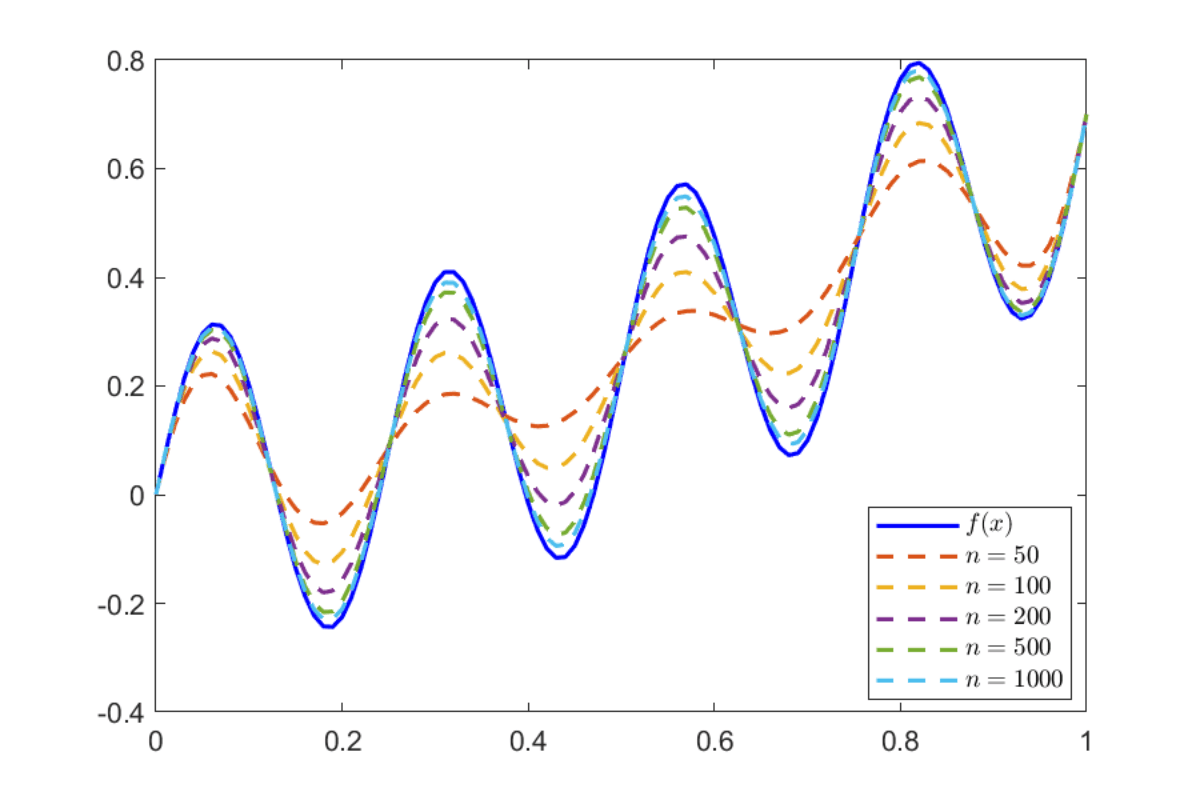
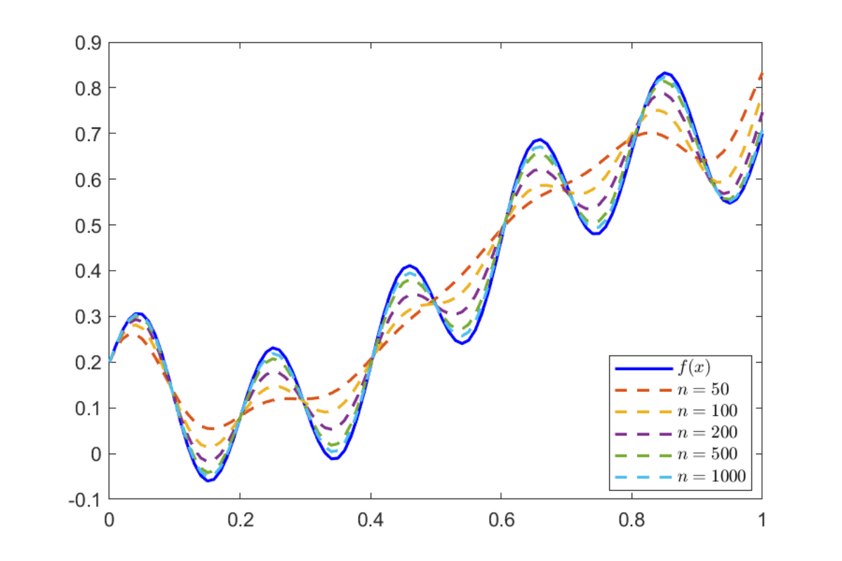
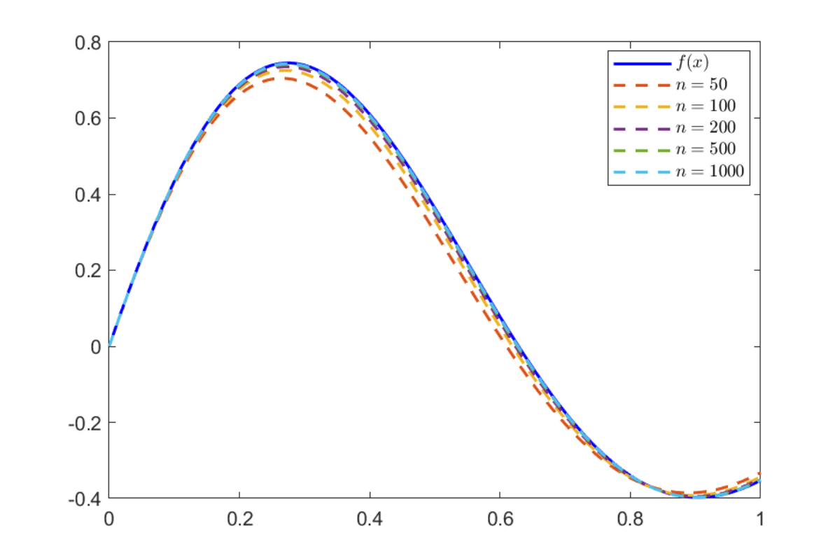
Based on the examples presented above, we consider the functions $f_1,f_2,f_3:[0,1]\to ℝ$, given by

$f_1(x)$ $\phantom{}=0.5x^2+0.3\sin (8\pi x)+0.2x,$

$f_2(x)$ $\phantom{}=0.3\sin (4\pi x)\cos (6\pi x)+0.5x^2+0.2,$

$f_3(x)$ $\phantom{}=\sin (5x)e^{-x},$

for $x\in [0,1]$. In Figure 1 we display the functions $f_i$ together with their corresponding operators ${ℳ}_{\lambda }^m{f}_i$, $i=1,2,3$ constructed using the functions $A_{\lambda ,k}$ and $B_{\lambda ,k,j}$ given in

• Example 13 for $i=1$,

• Example 14 for $i=2$,

• Example 15 for $i=3$, respectively.

Finally, Table 1 presents the maximum approximation errors for the operators ${ℳ}_{\lambda }^m{f}_i$, $i=1,2,3$, considering all the three cases given in Examples 13–15 and Table 2 presents the mean approximation errors. We consider the following parameters: $m=4$, $r_1=2,r_2=1,r_3=3,r_4=2$, $p=8$, $\lambda =n+p-R$ with $R=r_1+r_2+r_3+r_4$ and $n\in \{\mathrm{50,100,200,500},1000\}$.

$f_1\left(x\right)$

$f_2\left(x\right)$

$f_3\left(x\right)$

Figure 1. Functions $f_i,i=1,2,3$, and the corresponding ${ℳ}_{\lambda }^4{f}_i$ operators.

$f_i\backslash n$	Example	50	100	200	500	1000
$f_1$	1	$0.2549$	$0.1724$	$0.1014$	$0.0448$	$0.0231$
	2	$0.3118$	$0.1845$	$0.1041$	$0.0445$	$0.0229$
	3	$0.2742$	$0.1793$	$0.1059$	$0.0469$	$0.0243$
$f_2$	1	$0.1580$	$0.1142$	$0.0726$	$0.0339$	$0.0179$
	2	$0.1594$	$0.1197$	$0.0754$	$0.0349$	$0.0184$
	3	$0.1699$	$0.1252$	$0.0788$	$0.0367$	$0.0194$
$f_3$	1	$0.0472$	$0.0236$	$0.0118$	$0.0047$	$0.0024$
	2	$0.0411$	$0.0207$	$0.0106$	$0.0043$	$0.0022$
	3	$0.0631$	$0.0321$	$0.0162$	$0.0065$	$0.0033$

Table 1. Maximum approximation errors for ${ℳ}_{\lambda }^4{f}_i$, $i=1,2,3$.

$f_i\backslash n$	Example	50	100	200	500	1000
$f_1$	1	$0.1195$	$0.0767$	$0.0438$	$0.0190$	$0.0098$
	2	$0.1465$	$0.0912$	$0.0512$	$0.0219$	$0.0112$
	3	$0.1367$	$0.0864$	$0.0488$	$0.0211$	$0.0108$
$f_2$	1	$0.0724$	$0.0513$	$0.0314$	$0.0143$	$0.0075$
	2	$0.0841$	$0.0588$	$0.0353$	$0.0159$	$0.0083$
	3	$0.0798$	$0.0561$	$0.0340$	$0.0154$	$0.0080$
$f_3$	1	$0.0210$	$0.0105$	$0.0052$	$0.0021$	$0.0010$
	2	$0.0272$	$0.0139$	$0.0070$	$0.0028$	$0.0014$
	3	$0.0312$	$0.0157$	$0.0079$	$0.0032$	$0.0016$

Table 2. Mean approximation errors for ${ℳ}_{\lambda }^4{f}_i$, $i=1,2,3$.

5. A nonlinear extension with data-dependent weights

In this section, we present a nonlinear extension of the operator ${ℳ}_{\lambda }^m$ introduced in Section 2. By weakening the assumptions on the functions $A$ and $B$ defined in relation (6), we will consider that the weights appearing in the operator’s expression are themselves Bernstein-type operators. Thus, we obtain the operator ${ℳ}_{\lambda }^B$ defined by

(16) $${ℳ}_{\lambda }^{B}f(x)=\sum _{k=0}^{\lambda }{b}_{\lambda ,k}(x)\left[\left(1-{ℬ}_{n}f(x)\right)f\left(\frac{k}{n}\right)+{ℬ}_{n}f(x)f\left(\frac{k+r}{n}\right)\right],$$

where ${ℬ}_{n}f$ is the classical Bernstein operator given by (1) and $b_{\lambda ,k}$ are the Bernstein polynomials given by (2). Note that in this section we consider the particular case $m=1$ and then $\lambda =n+p-R$ reduces to $\lambda =n+p-r$, where $n,p,r\in \mathbb{N}$ with $p\ge 0$ and $n>2r$. It is clear that the operator is no longer linear, given the dependence of the weights on the function $f$. Moreover, the positivity of the operator is preserved only under certain conditions. Nevertheless, for the introduced operator, important properties in approximation theory can still be studied, as can be observed in this final section.

Remark 17.

Let ${ℳ}_{\lambda }^B$ be given by (16) and $f\in C[0,1+p]$. Then

$${ℳ}_{\lambda }^{B}f(0)=f(0)$$

and

$${ℳ}_{\lambda }^{B}f(1)=f\left(\frac{n+p}{n}\right).$$

In particular, if $p=0$, then ${ℳ}_{\lambda }^{B}f(1)=f(1).$ The proof of this result is very simple, according to the well-known properties of the Bernstein operator ${ℬ}_{n}f$.

Proposition 18.

Let $e_j(x)=x^j$, for every $j\in \{0,1,2\}$ and $x\in [0,1]$. Then

$${ℳ}_{\lambda }^B(e_0,x)=1$$

and

$${ℳ}_{\lambda }^B(e_1,x)=\frac{n+p}{n}x,$$

for all $x\in [0,1]$. Moreover,

$${ℳ}_{\lambda }^B(e_2,x)=\frac{1}{n^2}\left[\lambda x(1-x)+{\lambda }^2{x}^2+\left(2r\lambda x+r^2\right)\left(x^2+\frac{x(1-x)}{n}\right)\right],$$

for all $x\in [0,1]$.

Proof.

In view of Theorem 6 for $m=1$ and $B_{\lambda ,k,j}(x)={ℬ}_{n}f(x)$, for all $x\in [0,1]$, where ${ℬ}_{n}f$ is the Bernstein operator given by (1). ∎

It is not difficult to observe that for $p=0$ we obtain better results for the operator ${ℳ}_{\lambda }^B$ (in particular, we have that ${ℳ}_{\lambda }^B(e_1,x)=x$, for all $x\in [0,1]$) that are similar to those obtained for the Bernstein operator ${ℬ}_{n}f$ (see [21]).

Acknowledgements.

The authors thank the referee(s) for carefully reading the manuscript and providing helpful suggestions.

References

- [1]
- [2] G. Başcanbaz-Tunca, A. Erençin and F. Taşdelen, Some properties of Bernstein type Cheney and Sharma operators, Gen. Math., 24 (2016) nos.1-2, pp. 17-25.
- [3] S.N. Bernstein, Démonstration du théoréme de Weierstrass fondée sur le calcul des probabilités, Commun. Kharkov Math. Soc., 13 (1912/1913) no. 1, pp. 1-2.
- [4] T. Bostanci and G. Başcanbaz-Tunca, A Stancu type extension of Cheney and Sharma operator, J. Numer. Anal. Approx. Theory, 47 (2018) no. 2, pp. 124–134. https://doi.org/10.33993/jnaat472-1133
- [5] T. Cătinaş, Extension of Some Cheney-Sharma Type Operators to a Triangle With One Curved Side, Miskolc Math. Notes 21 (2020), pp. 101–111. https://dx.doi.org/10.18514/MMN.2020.2686
- [6] T. Cătinaş, Cheney–Sharma Type Operators on a Triangle with Straight Sides, Symmetry 14 (2022), no. 11, 2446. https://doi.org/10.3390/sym14112446
- [7] T. Cătinaş, A Stancu type extension of the Campiti-Metafune operator, J. Numer. Anal. Approx. Theory, 54 (2025) no. 2, pp. 229–236. DOI: 10.33993/jnaat542-1638
- [8] T. Cătinaş and I. Buda, An extension of the Cheney-Sharma operator of the first kind, J. Numer. Anal. Approx. Theory, 52 (2023) no. 2, pp. 172–181. https://doi.org/10.33993/jnaat522-1373
- [9] T. Cătinaş and D. Otrocol, Iterates of multivariate Cheney-Sharma operators, J. Comput. Anal. Appl. 15 (2013), No. 7, pp. 1240–1246.
- [10] T. Cătinaş and D. Otrocol, Iterates of Cheney-Sharma type operators on a triangle with curved side, J. Comput. Anal. Appl. 28 (2020), No. 4, pp. 737–744.
- [11] N. Çetin, A new generalization of complex Stancu operators, Math. Methods Appl. Sci. 42 (2019), pp 5582–5594.
- [12] N. Çetin, A new complex generalized Bernstein-Schurer operator, Carpathian J. Math., 37 (2021) no. 1, pp. 81-89.
- [13] N. Çetin and N.M. Mutlu, Complex generalized Stancu-Schurer operators, Math. Slovaca, 74 (2024) no.5, pp. 1215-1232.
- [14] E.W. Cheney and A. Sharma, On a generalization of Bernstein polynomials, Riv. Mat. Univ. Parma, 2 (1964), pp. 77-84.
- [15] S.G. Gal, Approximation by Complex Bernstein and Convolution Type Operators, Series on Concrete and Applicable Mathematics, vol. 8, World Scientific Publishing Co. Pte. Ltd., Hackensack, NJ, 2009.
- [16] E.S. Grigoriciuc, A Stancu type extension of the Cheney-Sharma Chlodovsky operators, J. Numer. Anal. Approx. Theory, 53 (2024) no. 1, pp. 103-117. DOI: 10.33993/jnaat531-1406
- [17] E.S. Grigoriciuc and A. Malina, A Stancu–Schurer type extension of higher order of the Cheney–Sharma operators, Math. Slovaca, 76 (2026) no. 1, pp. 225-244. DOI: 10.1515/ms-2025-1155
- [18] D. Miclăuş, The generalization of some results for Schurer and Schurer-Stancu operators, Rev. Anal. Numér. Théor. Approx., 40 (2011) no. 1, pp. 52-63.
- [19] F. Schurer, Linear positive operators in approximation theory, Math. Inst. Technol. Univ. Delft Rep., 1962.
- [20] D. Söylemez and F. Taşdelen, On Cheney-Sharma Chlodovsky operators, Bull. Math. Anal. Appl., 11 (2019) no. 1, pp. 36-43.
- [21] D.D. Stancu Quadrature formulas constructed by using certain linear positive operators, in Numerical Integration. ISNM 57: International Series of Numerical Mathematics, vol. 57, G. Hämmerlin, Ed., Basel, Birkhäuser, 1981, pp. 241-251.