Improving approximation via linear combinations of Bernstein operatorsThanks: ^∗1General Directorate of Basrah Education, Ministry of Education, 61001, Basrah, Iraq, e-mail: pgs.ali.jaddoa@uobasrah.edu.iq, ORCID: 0009-0009-4618-3395.Thanks: ²Department of Mathematics, University of Basrah, College of Education for Pure Sciences, Basrah, Iraq, e-mail: Hanadi.sattar@uobasrah.edu.iq, ORCID: 0000-0002-9989-2170. Thanks: ³Department of Computer Sciences, University of Basrah, College of Computer Sciences and Information Technology, Basrah, Iraq, e-mail: nasir.jasim@uobasrah.edu.iq, ORCID: 0000-0003-4545-4682.

Abstract.

In this paper we study linear combinations of Bernstein operators that admit the iterate ${𝒵}_n={ℬ}_n\circ {ℬ}_n$. Inside the span $\{{ℬ}_n,{ℬ}_{2n},{𝒵}_n\}$, which we adopt as an ansatz, requiring that constants be preserved and that the leading term of the second central moment vanish leaves a one-parameter family, of which Butzer’s operator ${𝒬}_n$ is the member using no iterate. The remaining parameter can annihilate the leading term of exactly one of the three central moments that enter the error at the leading order, so that the family has exactly three distinguished members; we study the one selected by the fourth moment, ${ℱ}_n$. We compute its moments and prove an error estimate of order $n^{-2}$ for $\phi \in C^4[0,1]$ with explicit constants, a refinement of it in which the contribution of ${\phi }^{(4)}$ is $o(n^{-2})$, an estimate in a modified fourth-order $K$-functional, uniform convergence on $C[0,1]$, and a Voronovskaja-type formula. The comparison with ${𝒬}_n$ is the point of the construction: the choice removes the ${\phi }^{(4)}$ term of the asymptotic error and introduces a ${\phi }^{\prime \prime }$ term, so that neither operator dominates the other. Numerical examples illustrate both regimes.

1. Introduction

In 1912, Bernstein [3] introduced a very famous operator in approximation theory. For a function $\phi \in C[0,1]$, it is defined as:

(1) $${ℬ}_n(\phi ,y)=\sum _{w=0}^n\left(\genfrac{}{}{0pt}{}{n}{w}\right)y^w{(1-y)}^{n-w}\phi \left(\frac{w}{n}\right),y\in [0,1].$$

This operator is widely used because of its simple binomial structure and its ability to preserve the shape of the function; however, its main drawback is the slow rate of convergence, which is only $𝒪(n^{-1})$, and this motivates the search for modified operators with better approximation behaviour. To fix this speed problem, various modification techniques have been developed in the literature. One common approach, initiated by Butzer in 1953 [4], involves forming linear combinations of Bernstein operators. This technique effectively reduces lower-order errors and accelerates the approximation process; the systematic theory of such combinations, together with the moduli of smoothness appropriate to them, is developed in [7]. A classic example is given by

(2) $${𝒬}_n=2{ℬ}_{2n}-{ℬ}_n,$$

which achieves a convergence rate of $𝒪(n^{-2})$. Combinations of arbitrary order $𝒪(n^{-k})$ are obtained in the same manner and have long been available; see May [14] for the general exponential-type framework and Ditzian and Ivanov [6] for the converse theory that accompanies them.

Another approach relies on iterating the operator, denoted as ${ℬ}_n^k$. Kelisky and Rivlin [11] were among the first to investigate this, followed by important results on behaviour and stability from Micchelli [15], Raşa [18], and recently Acu and Raşa [1]. Parallel to these developments, significant effort has been directed towards designing operators that reproduce specific functions or incorporate shape parameters to enhance modelling flexibility and accuracy [12, 10, 22, 16, 21, 17, 23]. A different device for raising the order, which we do not pursue here, is that of quasi-interpolants [20].

The combination studied here is not postulated but obtained from two structural requirements. Writing ${\psi }_y(t)=t-y$, consider all combinations, taken here as our ansatz,

$$L=a{ℬ}_{2n}+b{ℬ}_n+c{𝒵}_n,{𝒵}_n={ℬ}_n\circ {ℬ}_n,$$

subject to two structural requirements: preservation of constants, $a+b+c=1$, and the vanishing of the $𝒪(n^{-1})$ term of $L({\psi }_y^2,y)$, which reads $\frac{a}{2}+b+2c=0$. These two linear conditions leave one free parameter; solving them gives the one-parameter family

(3) $$L_c=(2+2c){ℬ}_{2n}-(1+3c){ℬ}_n+c{𝒵}_n,c\in ℝ,$$

whose member $c=0$ is exactly Butzer’s operator (2), in which the iterate plays no role; every $c\ne 0$ is a genuine use of iteration. Equivalently, writing $U_n=2{ℬ}_n-{𝒵}_n$ for the Boolean sum of the Bernstein operator [18], the family (3) is the affine line

$$L_c=(1+c){𝒬}_n-c{U}_n,$$

through Butzer’s operator and $U_n$, the parameter $c$ being the position on it.

All members of (3) share the approximation order $𝒪(n^{-2})$, so the parameter must be fixed by a finer criterion, and the central moments provide one. By Section 2, the leading term of $L_c({\psi }_y^m,y)$ is, for every $m\ge 2$, an affine function of $c$ with a single root; at the order $n^{-2}$ exactly three moments contribute, those of $m=2,3,4$, with roots $c=0$, $c=\frac{1}{5}$ and $c=\frac{1}{3}$. The case $m=2$ is no exception: the two conditions defining (3) remove the $𝒪(n^{-1})$ term of $L_c({\psi }_y^2,y)$ for every $c$, and what remains, $cy(y-1)n^{-2}$, vanishes only for $c=0$. The single free parameter can annihilate exactly one of the three terms, and no choice annihilates two, so (3) has exactly three distinguished members, $L_0={𝒬}_n$, $L_{1/5}$ and $L_{1/3}$, the first being Butzer’s operator and the other two new. We study the member selected by the fourth moment, the one that removes the term of highest differential order, and it is

(4) $${ℱ}_n(\phi ,y):=L_{1/3}(\phi ,y)=\frac{8}{3}{ℬ}_{2n}(\phi ,y)-2{ℬ}_n(\phi ,y)+\frac{1}{3}{𝒵}_n(\phi ,y),$$

for which the fourth central moment satisfies ${\mathrm{\Omega }}_{n,4}=𝒪(n^{-3})$, one power better than for a generic member of the family (here ${\mathrm{\Omega }}_{n,m}$ denotes the $m$-th central moment of ${ℱ}_n$; see Section 2). Throughout, $\Vert \phi \Vert ={\max }_{y\in [0,1]}|\phi (y)|$.

This choice is not a uniform improvement, and we do not claim it as one. The same computation shows that $c=0$ is the unique member of (3) reproducing $e_2$, and the unique one whose asymptotic error carries no ${\phi }^{\prime \prime }$ term. Admitting the iterate therefore trades a second-order term for the annihilation of a fourth-order one, so that ${ℱ}_n$ is advantageous precisely on functions with large high-order derivatives and inferior to ${𝒬}_n$ on ordinary smooth ones. We note at the outset that ${ℱ}_n$, like ${𝒬}_n$, is not a positive operator, so that the shape-preserving properties of ${ℬ}_n$ are not inherited (Section 2). The trade-off is made quantitative in Section 3 and confirmed numerically in Section 4 .

The paper is organized as follows. Section 2 records the moments of ${ℬ}_n$ and ${𝒵}_n$, establishes the selection identities of Section 2 and the choice $c=\frac{1}{3}$, and computes the moments and central moments of ${ℱ}_n$. Section 3 contains the quantitative error estimates and a Voronovskaja-type theorem for $\phi \in C^4[0,1]$, together with the explicit comparison with ${𝒬}_n$; the quantitative form of the Voronovskaja formula, for which we refer to Gonska [9], is not pursued here. Section 4 reports numerical experiments on both smooth and non-smooth test functions.

2. Preliminaries and Auxiliary Results

In this section we collect the auxiliary results needed later. We first record the moments and central moments of the classical Bernstein operator and of its second iterate ${𝒵}_n={ℬ}_n\circ {ℬ}_n$, then those of ${ℱ}_n$, and finally establish, in Section 2, the asymptotic identities on which the selection of $c=\frac{1}{3}$ rests.

Lemma .

For each $i\in {\mathbb{N}}_0$ let $e_i(t)=t^i$; the operators map functions of $t$ to functions of $y$. Then, for the classical Bernstein operator ${ℬ}_n$ and the composition ${𝒵}_n={ℬ}_n\circ {ℬ}_n$, the following equalities hold for any $y\in [0,1]$:

${ℬ}_n(e_0,y)={𝒵}_n(e_0,y)=1,{ℬ}_n(e_1,y)={𝒵}_n(e_1,y)=y,{ℬ}_n(e_2,y)=y^2+\frac{y(1-y)}{n},$

${𝒵}_n(e_2,y)=y^2+\frac{(2n-1)y(1-y)}{n^2},$

${ℬ}_n(e_3,y)=y^3+\frac{3y^2(1-y)}{n}+\frac{y(1-y)(1-2y)}{n^2},$

${𝒵}_n(e_3,y)=y^3+\frac{6y^2(1-y)}{n}+\frac{13y^3-18y^2+5y}{n^2}+\frac{-12y^3+18y^2-6y}{n^3}$

$+\frac{4y^3-6y^2+2y}{n^4},$

${ℬ}_n(e_4,y)=y^4-\frac{6y^3(y-1)}{n}+\frac{y^2(y-1)(11y-7)}{n^2}-\frac{y(y-1)(6y^2-6y+1)}{n^3},$

${𝒵}_n(e_4,y)=y^4-\frac{12y^3(y-1)}{n}+\frac{2y^2(y-1)(29y-16)}{n^2}$

$-\frac{3y(y-1)(48y^2-40y+5)}{n^3}+\frac{y(y-1)(193y^2-185y+31)}{n^4}$

$-\frac{y(y-1)(132y^2-132y+23)}{n^5}+\frac{6y(y-1)(6y^2-6y+1)}{n^6}.$

The corresponding formulas for ${ℬ}_{2n}$ follow by replacing $n$ with $2n$.

Proof.

The moments of ${ℬ}_n$ are standard [13]; explicitly,

$${ℬ}_n(e_m,y)=n^{-m}\sum _{k=0}^{m}S(m,k)n^{\underset{¯}{k}}{y}^k,$$

where $S(m,k)$ denote the Stirling numbers of the second kind and $n^{\underset{¯}{k}}=n(n-1)\cdots (n-k+1)$ is the falling factorial. Since ${ℬ}_n(e_m,\cdot )$ is a polynomial of degree $m$, the moments of the composition are obtained by substituting that polynomial into the outer operator and applying the same formula termwise:

$${𝒵}_n(e_m,y)=\sum _{j=0}^m{\left[{ℬ}_n(e_m,\cdot )\right]}_j{ℬ}_n(e_j,y),$$

${[\cdot ]}_j$ denoting the coefficient of $s^j$. This is consistent with the properties of iterates established in [15, 8]. ∎

Lemma .

The central moments of ${ℬ}_n$ and ${𝒵}_n$ are given by:

${ℬ}_n({\psi }_y^0,y)={𝒵}_n({\psi }_y^0,y)=1,{ℬ}_n({\psi }_y^1,y)={𝒵}_n({\psi }_y^1,y)=0,$

${ℬ}_n({\psi }_y^2,y)=\frac{y(1-y)}{n},{𝒵}_n({\psi }_y^2,y)=\frac{(2n-1)y(1-y)}{n^2},$

${ℬ}_n({\psi }_y^3,y)=\frac{y(2y^2-3y+1)}{n^2},{𝒵}_n({\psi }_y^3,y)=\frac{(5n^2-6n+2)y(1-y)(1-2y)}{n^4},$

${ℬ}_n({\psi }_y^4,y)=\frac{3y^2{(y-1)}^2}{n^2}-\frac{y(y-1)(6y^2-6y+1)}{n^3},$

${𝒵}_n({\psi }_y^4,y)=\frac{12y^2{(y-1)}^2}{n^2}-\frac{3y(y-1)(32y^2-32y+5)}{n^3}$

$+\frac{y(y-1)(177y^2-177y+31)}{n^4}-\frac{y(y-1)(132y^2-132y+23)}{n^5}$

$+\frac{6y(y-1)(6y^2-6y+1)}{n^6}.$

Again, the formulas for ${ℬ}_{2n}$ follow by replacing $n$ with $2n$. In particular, writing ${\sigma }^2={\sigma }^2(y)=y(1-y)$, ${𝒵}_n({\psi }_y^2,y)=2{\sigma }^2{n}^{-1}+𝒪(n^{-2})$ and ${𝒵}_n({\psi }_y^4,y)=3{(2{\sigma }^2)}^2{n}^{-2}+𝒪(n^{-3})$: the variance of the iterate is asymptotically twice that of ${ℬ}_n$.

Proof.

The results follow by expressing the central moments in terms of the raw moments of Section 2, using the linearity of the operators and the binomial expansion of ${(t-y)}^m$. ∎

Lemma .

Let ${ℱ}_n$ be the operator defined in (4). Then for $y\in [0,1]$:

$(i){ℱ}_n(e_0,y)=1,(\mathrm{ii}){ℱ}_n(e_1,y)=y,(\mathrm{iii}){ℱ}_n(e_2,y)=y^2+\frac{y(y-1)}{3n^2},$

$(\mathrm{iv}){ℱ}_n(e_3,y)=y^3+\frac{y(y-1)(5y-1)}{3n^2}-\frac{2y(y-1)(2y-1)}{n^3}$

$+\frac{2y(y-1)(2y-1)}{3n^4}.$

Proof.

The proof follows from the linearity of ${ℱ}_n$ and the moments of the component operators established in Section 2. Since ${ℬ}_n$, ${ℬ}_{2n}$ and ${𝒵}_n$ preserve linear functions, we immediately obtain

$$(i){ℱ}_n(e_0,y)=\frac{8}{3}{ℬ}_{2n}(e_0,y)-2{ℬ}_n(e_0,y)+\frac{1}{3}{𝒵}_n(e_0,y)=\frac{8}{3}-2+\frac{1}{3}=1,$$

$$(\mathrm{ii}){ℱ}_n(e_1,y)=\frac{8}{3}{ℬ}_{2n}(e_1,y)-2{ℬ}_n(e_1,y)+\frac{1}{3}{𝒵}_n(e_1,y)=\frac{8y}{3}-2y+\frac{y}{3}=y.$$

$(\mathrm{iii}){ℱ}_n(e_2,y)$ $\phantom{}=\frac{8}{3}{ℬ}_{2n}(e_2,y)-2{ℬ}_n(e_2,y)+\frac{1}{3}{𝒵}_n(e_2,y)$

$\phantom{}=\frac{8}{3}\left(y^2+\frac{y(1-y)}{2n}\right)-2\left(y^2+\frac{y(1-y)}{n}\right)$

$+\frac{1}{3}\left(y^2+\frac{(2n-1)y(1-y)}{n^2}\right)$

$\phantom{}=y^2+y(1-y)\left[\frac{4}{3n}-\frac{2}{n}+\frac{2n-1}{3n^2}\right]$

$\phantom{}=y^2+y(1-y)\frac{4n-6n+2n-1}{3n^2}=y^2+\frac{y(y-1)}{3n^2}.$

For $(\mathrm{iv})$, substituting the third moments of Section 2 and using
${ℬ}_{2n}(e_3,y)=y^3+\frac{3}{2}{y}^2(1-y)n^{-1}+\frac{1}{4}y(1-y)(1-2y)n^{-2}$ gives

${ℱ}_n(e_3,y)-y^3$ $=y^2(-y)[\frac{8}{3}\cdot \frac{3}{2}-\cdot 3+\frac{1}{3}\cdot 6]\frac{1}{n}+y(-y)(-2y)[\frac{8}{3}\cdot \frac{1}{4}-2]\frac{1}{n^2}$

$+\frac{1}{3}\left[\frac{13y^3-18y^2+5y}{n^2}+\frac{-12y^3+18y^2-6y}{n^3}+\frac{4y^3-6y^2+2y}{n^4}\right].$

The bracket multiplying $n^{-1}$ vanishes, and collecting the remaining terms yields the stated expression. ∎

Lemma .

Let ${\mathrm{\Omega }}_{n,m}(y)={ℱ}_n({\psi }_y^m,y)$ be the $m$-th central moment of ${ℱ}_n$. Then:

$(i){\mathrm{\Omega }}_{n,0}(y)=1,(\mathrm{ii}){\mathrm{\Omega }}_{n,1}(y)=0,(\mathrm{iii}){\mathrm{\Omega }}_{n,2}(y)=\frac{y(y-1)}{3n^2},$

$(\mathrm{iv}){\mathrm{\Omega }}_{n,3}(y)=\frac{y(y-1)(2y-1)}{3n^2}-\frac{2y(y-1)(2y-1)}{n^3}+\frac{2y(y-1)(2y-1)}{3n^4},$

$(v){\mathrm{\Omega }}_{n,4}(y)=-\frac{2y(y-1)(33y^2-33y+5)}{3n^3}+\frac{y(y-1)(177y^2-177y+31)}{3n^4}$

$+\frac{-y(y-1)(132y^2-132y+23)}{3n^5}+\frac{2y(y-1)(6y^2-6y+1)}{n^6}.$

In particular ${\mathrm{\Omega }}_{n,4}(y)=𝒪(n^{-3})$ uniformly on $[0,1]$.

Proof.

Using ${\mathrm{\Omega }}_{n,m}(y)={\sum }_{j=0}^m\left(\genfrac{}{}{0pt}{}{m}{j}\right){(-y)}^{m-j}{ℱ}_n(e_j,y)$ and substituting the values of Section 2 for $m\le 3$, and those of Section 2 for $m=4$, the results follow. Specifically, for $m=2$,

${\mathrm{\Omega }}_{n,2}(y)$ $\phantom{}={ℱ}_n(e_2,y)-2y{ℱ}_n(e_1,y)+y^2{ℱ}_n(e_0,y)$

$\phantom{}=\left(y^2+\frac{y(y-1)}{3n^2}\right)-2y^2+y^2=\frac{y(y-1)}{3n^2},$

and for $m=4$ the four displayed terms are obtained from the fourth moments of ${ℬ}_{2n}$, ${ℬ}_n$ and ${𝒵}_n$ recorded in Section 2. ∎

Lemma .

Let $c\in ℝ$ and ${\sigma }^2={\sigma }^2(y)=y(1-y)$.

1. Expansions. For every $k\ge 1$

   $${ℬ}_n({\psi }_y^{2k},y)=(2k-1)!!\frac{{\sigma }^{2k}}{n^k}+𝒪(n^{-k-1}),$$

   $${𝒵}_n({\psi }_y^{2k},y)=2^k(2k-1)!!\frac{{\sigma }^{2k}}{n^k}+𝒪(n^{-k-1}),$$

   and

   $${ℬ}_n({\psi }_y^{2k+1},y)=\frac{1}{3}k(2k+1)!!\frac{{\sigma }^{2k}(1-2y)}{n^{k+1}}+𝒪(n^{-k-2}),$$

   $${𝒵}_n({\psi }_y^{2k+1},y)=5\cdot 2^{k-1}\cdot \frac{1}{3}k(2k+1)!!\frac{{\sigma }^{2k}(1-2y)}{n^{k+1}}+𝒪(n^{-k-2}),$$

   the corresponding expansions for ${ℬ}_{2n}$ following on replacing $n$ by $2n$, that is on dividing them by $2^k$ and $2^{k+1}$ respectively.

2. Even orders. For every $k\ge 1$

   $$L_c({\psi }_y^{2k},y)=(2k-1)!!\frac{{\sigma }^{2k}}{n^k}{\kappa }_k(c)+𝒪(n^{-k-1}),{\kappa }_k(c)=\frac{2+2c}{2^k}-(1+3c)+c{\mathrm{\hspace{0.17em}2}}^k,$$

   where ${\kappa }_1(c)\equiv 0$, the second central moment being exact,

   $$L_c({\psi }_y^2,y)=cy(y-1)n^{-2},$$

   and where, for $k\ge 2$, ${\kappa }_k(c)=0$ if and only if $c={(2^k-1)}^{-1}$.

3. Odd orders. For every $k\ge 1$

   $L_c({\psi }_y^{2k+1},y)=\frac{1}{3}k(2k+1)!!\frac{{\sigma }^{2k}(1-2y)}{n^{k+1}}{\lambda }_k(c)+𝒪(n^{-k-2}),$

   ${\lambda }_k(c)=\frac{2+2c}{2^{k+1}}-(1+3c)+5c{\mathrm{\hspace{0.17em}2}}^{k-1}.$

   Here ${\lambda }_k(c)=0$ if and only if $c=2(2^k-1)/(5\cdot 4^k-6\cdot 2^k+2)$.

4. In particular, for ${ℱ}_n=L_{1/3}$, ${\mathrm{\Omega }}_{n,m}(y)=O\left(n^{-\lceil m/2\rceil }\right)$ for $m\ge 2$, the improved order $O\left(n^{-\lceil m/2\rceil -1}\right)$ holding only for $m\in \{2,4\}$.

Proof.

The expansions. Let $T_{n,m}(y)={ℬ}_n({\psi }_y^m,y)$; these satisfy the classical recurrence [13]

$$T_{n,m+1}(y)=\frac{{\sigma }^2}{n}\left[T_{n,m}^{\prime }(y)+m{T}_{n,m-1}(y)\right],T_{n,0}=1,T_{n,1}=0.$$

Induction on $m$ shows that $T_{n,m}$ is a polynomial in $y$ all of whose coefficients are $𝒪(n^{-\lceil m/2\rceil })$, so that differentiation does not change their order, and gives

$$T_{n,2k}=(2k-1)!!\frac{{\sigma }^{2k}}{n^k}+𝒪(n^{-k-1}),T_{n,2k+1}={\mu }_k\frac{{\sigma }^{2k}(1-2y)}{n^{k+1}}+𝒪(n^{-k-2}),$$

with ${\mu }_k=k(2k-1)!!+2k{\mu }_{k-1}$, that is ${\mu }_k=\frac{1}{3}k(2k+1)!!$; the base cases $T_{n,2}={\sigma }^2{n}^{-1}$ and $T_{n,3}={\sigma }^2(1-2y)n^{-2}$ are exact. Replacing $n$ by $2n$ gives the expansions for ${ℬ}_{2n}$, dividing them by $2^k$ and $2^{k+1}$ respectively. For the iterate, write ${(t-y)}^m={\sum }_j\left(\genfrac{}{}{0pt}{}{m}{j}\right){(t-s)}^j{(s-y)}^{m-j}$ and apply the inner operator at $s$, then the outer one at $y$:

$${𝒵}_n({\psi }_y^m;y)=\sum _{j=0}^m\left(\genfrac{}{}{0pt}{}{m}{j}\right){ℬ}_n({(\cdot -y)}^{m-j}{T}_{n,j}(\cdot );y).$$

Since $T_{n,j}=𝒪\left(n^{-\lceil j/2\rceil }\right)$ and ${ℬ}_n({\psi }_y^i,y)=𝒪\left(n^{-\lceil i/2\rceil }\right)$, expanding $T_{n,j}$ about $y$ shows that the term of index $j$ and Taylor order $r$ is $O\left(n^{-\lceil j/2\rceil -\lceil (m-j+r)/2\rceil }\right)$; this exponent is never below $\lceil m/2\rceil$, and equality determines the terms that contribute at leading order. When $m=2k$ is even, replacing $T_{n,j}(s)$ by $T_{n,j}(y)$ suffices, as the Taylor correction $T_{n,j}^{\prime }(y){ℬ}_n({\psi }_y^{m-j+1},y)$ is one power of $n$ smaller. When $m=2k+1$ is odd, for each even index $j=2r$ the main term $T_{n,2r}(y){ℬ}_n({\psi }_y^{2k+1-2r},y)$ and the Taylor derivative correction $T_{n,2r}^{\prime }(y){ℬ}_n({\psi }_y^{2k+2-2r},y)$ both contribute at the leading order $𝒪(n^{-k-1})$. Summing these combined contributions over all indices yields the factor $2^k$ for $m=2k$ and $5\cdot 2^{k-1}$ for $m=2k+1$, completing the proof of (i); the cases $m=2,3,4$ of Section 2 confirm the factors $2$, $5$ and $4$.

(ii). Substituting the three expansions into (3) and collecting the coefficient of $(2k-1)!!{\sigma }^{2k}{n}^{-k}$ yields ${\kappa }_k(c)$. Multiplying ${\kappa }_k(c)=0$ by $2^k$ gives
$c(4^k-3\cdot 2^k+2)=2^k-2$, and since $4^k-3\cdot 2^k+2=(2^k-1)(2^k-2)$ we obtain $c={(2^k-1)}^{-1}$ for $k\ge 2$, both sides vanishing identically for $k=1$. There the moment is exact: by Section 2,

$$L_c({\psi }_y^2,y)={\sigma }^2\left[\frac{2+2c}{2n}-\frac{1+3c}{n}+c\frac{2n-1}{n^2}\right]=-\frac{c{\sigma }^2}{n^2}=\frac{cy(y-1)}{n^2}.$$

(iii). The same substitution, with the factors $2^{-(k+1)}$ and $5\cdot 2^{k-1}$ in place of $2^{-k}$ and $2^k$, yields ${\lambda }_k(c)$; multiplying ${\lambda }_k(c)=0$ by $2^{k+1}$ gives
$c(5\cdot 4^k-6\cdot 2^k+2)=2^{k+1}-2$, whence the root, the coefficient of $c$ being positive. Section 2 confirms the case $k=1$, where ${\lambda }_1(c)=\frac{1}{2}(5c-1)$.

(iv). By part (i) each of the three components of (4) has $m$-th central moment $𝒪(n^{-\lceil m/2\rceil })$, so the triangle inequality gives ${\mathrm{\Omega }}_{n,m}=𝒪(n^{-\lceil m/2\rceil })$ for every $m\ge 2$. For $c=\frac{1}{3}$ part (ii) gives ${\kappa }_k=\frac{8}{3}{2}^{-k}-2+\frac{1}{3}{2}^k$, so that ${\kappa }_1={\kappa }_2=0$, ${\kappa }_3=1$, ${\kappa }_4=\frac{7}{2}$ and ${\kappa }_k>0$ for $k\ge 3$: the gain of one power of $n$ occurs for $m=2$ and $m=4$ and fails from $m=6$ onwards. By part (iii), ${\lambda }_1(\frac{1}{3})=\frac{1}{3}\ne 0$ and ${\lambda }_k(\frac{1}{3})>0$ for $k\ge 1$, so no odd moment gains a power. ∎

Remark .

Three consequences for the family (3).

(i) By Section 2(ii), $L_c({\psi }_y^2,y)=cy(y-1)n^{-2}$ exactly, so ${𝒬}_n=L_0$ is the only member reproducing $e_2$ and the only one whose asymptotic error carries no ${\phi }^{\prime \prime }$ term; $L_{1/5}$ and ${ℱ}_n=L_{1/3}$ are the members singled out in the same way by the third and by the fourth moment.

(ii) No member is positive, ${𝒬}_n$ included. For $c>0$ the second central moment is negative on $(0,1)$; for $c\le 0$ it is not, and one uses the fourth instead, $L_c({\psi }_y^4,y)=\frac{3}{2}(3c-1)y^2{(y-1)}^2{n}^{-2}+𝒪(n^{-3})$ with $\frac{3}{2}(3c-1)\le -\frac{3}{2}$. Consequently no Korovkin-type argument is available – convergence is obtained in Section 3 through the $K$-functional instead – and ${ℱ}_n$ preserves neither monotonicity nor convexity.

(iii) Each member is nevertheless a combination of the positive operators ${ℬ}_{2n}$, ${ℬ}_n$ and ${𝒵}_n$, so that

$$|L_c(g,y)|\le \phantom{}|2+2c|{ℬ}_{2n}(|g|,y)+|1+3c|{ℬ}_n(|g|,y)+|c|{𝒵}_n(|g|,y),g\in C[0,1],$$

and in particular $|{ℱ}_n(g,y)|\le \frac{8}{3}{ℬ}_{2n}(|g|,y)+2{ℬ}_n(|g|,y)+\frac{1}{3}{𝒵}_n(|g|,y)$. Every estimate below rests on this inequality, the Cauchy–Schwarz inequality [2] being applied to each component separately; we refer to it as passing to the three positive components.

3. Main Results

In this section we first establish the uniform boundedness of ${ℱ}_n$, then record in Section 3 the Taylor decomposition on which all the direct estimates rest. From it we deduce a direct estimate for $\phi \in C^2[0,1]$, the quantitative $𝒪(n^{-2})$ estimate for $\phi \in C^4[0,1]$ with explicit constants, and a refinement of the latter in which the contribution of ${\phi }^{(4)}$ is $o(n^{-2})$. We then give an estimate in a modified fourth-order $K$-functional and derive a Voronovskaja-type asymptotic formula for the whole family, from which the comparison between ${ℱ}_n$ and Butzer’s operator ${𝒬}_n$ follows explicitly.

Theorem 1.

The operators ${ℱ}_n$ are uniformly bounded on $C[0,1]$:

$$|{ℱ}_n(\phi ,y)|\le 5\Vert \phi \Vert (\phi \in C[0,1],y\in [0,1],n\in \mathbb{N}),$$

that is, ${\Vert {ℱ}_n\Vert }_{C\to C}\le 5$.

Proof.

By (4) and the triangle inequality,

$\left|{ℱ}_n(\phi ,y)\right|$ $\phantom{}=\left|\frac{8}{3}{ℬ}_{2n}(\phi ,y)-2{ℬ}_n(\phi ,y)+\frac{1}{3}{𝒵}_n(\phi ,y)\right|$

$\phantom{}\le \frac{8}{3}\left|{ℬ}_{2n}(\phi ,y)\right|+2\left|{ℬ}_n(\phi ,y)\right|+\frac{1}{3}\left|{𝒵}_n(\phi ,y)\right|.$

Each of ${ℬ}_n$, ${ℬ}_{2n}$ and ${𝒵}_n$ is a positive linear operator reproducing constants, so that

$$\left|{ℬ}_n(\phi ,y)\right|\le \Vert \phi \Vert ,\left|{ℬ}_{2n}(\phi ,y)\right|\le \Vert \phi \Vert \text{and}\left|{𝒵}_n(\phi ,y)\right|\le \Vert \phi \Vert .$$

Substituting these bounds back into the inequality:

$|{ℱ}_n(\phi ,y)|$ $\le |\phi |\left(\frac{8}{3}+2+\frac{1}{3}\right)=5\Vert \phi \Vert .$

∎

Lemma .

Let $c\in ℝ$, let $r\ge 2$ be even and $\phi \in C^r[0,1]$. Then, for every $y\in [0,1]$,

(5) $${Ł}_c(\phi ,y)-\phi (y)=\sum _{j=2}^r\frac{{\phi }^{(j)}(y)}{j!}{L}_c({\psi }_y^j,y)+L_c({\psi }_y^r{\epsilon }_y,y),$$

where ${\epsilon }_y$ is defined for $t\ne y$ by

$${\epsilon }_y(t)={\psi }_y^{-r}\left(\phi (t)-\sum _{j=0}^r\frac{{\psi }_y^j}{j!}{\phi }^{(j)}(y)\right),{\epsilon }_y(y):=0.$$

Being a quotient of continuous functions away from $t=y$, and satisfying ${\epsilon }_y(t)=\frac{1}{r!}\left({\phi }^{(r)}({\xi }_t)-{\phi }^{(r)}(y)\right)$ for some ${\xi }_t$ between $y$ and $t$, the function ${\epsilon }_y$ is continuous on the whole of $[0,1]$ and $|{\epsilon }_y(t)|\le \frac{1}{r!}\omega ({\phi }^{(r)},|t-y|)$. Moreover, with $C_r$ a constant depending only on $r$ and $c$,

(6) $$\left|L_c({\psi }_y^r{\epsilon }_y;y)\right|\le \frac{C_r}{n^{r/2}}\omega ({\phi }^{(r)},n^{-1/2}).$$

Proof.

Taylor’s formula with Lagrange remainder [19] gives $\phi (t)=\phantom{}$ ${\sum }_{j=0}^r\frac{{\psi }_y^j}{j!}{\phi }^{(j)}(y)+{\psi }_y^r{\epsilon }_y(t)$ with ${\epsilon }_y$ as stated; applying $L_c$, which reproduces constants and linear functions yields (5).

For (6) put $\delta =n{}^{-1/2}$. From $\omega ({\phi }^{(r)},\lambda \delta )\le (1+\lambda )\omega ({\phi }^{(r)},\delta )$,

$$|{\epsilon }_y(t)|\le \frac{\omega ({\phi }^{(r)},\delta )}{r!}\left(1+\frac{|t-y|}{\delta }\right),$$

so that, $𝒜$ denoting any of ${ℬ}_{2n}$, ${ℬ}_n$, ${𝒵}_n$ and $r$ being even,

$$𝒜({\psi }_y^r|{\epsilon }_y|,y)\le \frac{\omega ({\phi }^{(r)},\delta )}{r!}\left[𝒜({\psi }_y^r,y)+{\delta }^{-1}\sqrt{𝒜({\psi }_y^r,y)𝒜({\psi }_y^{r+2},y)}\right],$$

by the Cauchy–Schwarz inequality [2] applied to ${|{\psi }_y|}^{r+1}={|{\psi }_y|}^{r/2}\cdot {|{\psi }_y|}^{(r+2)/2}$. By Section 2(i) the two moments are $𝒪(n^{-r/2})$ and $𝒪(n^{-r/2-1})$, so the bracket is $𝒪(n^{-r/2})+n^{1/2}𝒪(n^{-r/2-1/2})=𝒪(n^{-r/2})$. Passing to the three positive components (Section 2(iii)) gives (6). ∎

Theorem 2.

Let $\phi \in C^2[0,1]$. Then, with $C_2$ the constant of Section 3 for $r=2$ and $c=\frac{1}{3}$

$$|{ℱ}_n(\phi ;y)-\phi (y)|\le \frac{\Vert {\phi }^{\prime \prime }\Vert }{24n^2}+\frac{C_2}{n}\omega ({\phi }^{\prime \prime },n^{-1/2}),y\in [0,1],$$

$\omega$ denoting the modulus of continuity. In particular $\Vert {ℱ}_n\phi -\phi \Vert =o(n^{-1})$.

Proof.

Apply Section 3 with $r=2$: the sum in (5) reduces to $\frac{1}{2}{\phi }^{\prime \prime }(y){\mathrm{\Omega }}_{n,2}(y)$, and $|{\mathrm{\Omega }}_{n,2}(y)|=|y(y-1)|/(3n^2)\le 1/(12n^2)$ by Section 2(iii), whence the first term. The second is $\le C_2{n}^{-1}\omega ({\phi }^{\prime \prime },n^{-1/2})$ by (6), and $\omega ({\phi }^{\prime \prime },n^{-1/2})\to 0$ gives the final assertion. ∎

Remark .

Neither of the two constants is sharp. The value $5$ cannot be lowered to $1$, a linear operator reproducing constants having norm $1$ exactly when it is positive; but numerically ${\Vert {ℱ}_n\Vert }_{C\to C}$ stays below $1.77$, and any sharpening of Theorem 1 improves the constant $6=1+5$ of Theorem 5 in the same proportion. The rate $o(n^{-1})$ of Theorem 2 is likewise not $𝒪(n^{-2})$: its second term is controlled only by the modulus of continuity of ${\phi }^{\prime \prime }$, and the order $n^{-2}$ of Theorem 3 needs two further derivatives.

Theorem 3.

Let $\phi \in C^4[0,1]$ and $n\ge 6$. Then

$$\Vert {ℱ}_n\phi -\phi \Vert \le \frac{1}{n^2}\left(\frac{\Vert {\phi }^{\prime \prime }\Vert }{24}+\frac{\sqrt{3}\Vert {\phi }^{\prime \prime \prime }\Vert }{324}+\frac{\Vert {\phi }^{(4)}\Vert }{32}\right).$$

In particular $\Vert {ℱ}_n\phi -\phi \Vert =𝒪(n^{-2})$ with explicit constants.

Proof.

Apply Section 3 with $r=4,c=\frac{1}{3}$ and recombine the last two terms of (5): since $\frac{1}{24}{\psi }_y^4{\phi }^{(4)}(y)+{\psi }_y^4{\epsilon }_y=\frac{1}{24}{\psi }_y^4{\phi }^{(4)}({\xi }_t)=\phantom{}:R_y(t)$,

(7) $${ℱ}_n(\phi ,y)-\phi (y)=\frac{{\phi }^{\prime \prime }(y)}{2}{\mathrm{\Omega }}_{n,2}(y)+\frac{{\phi }^{\prime \prime \prime }(y)}{6}{\mathrm{\Omega }}_{n,3}(y)+{ℱ}_n(R_y,y).$$

First term. As in Theorem 2, $|{\mathrm{\Omega }}_{n,2}(y)|\le 1/(12n^2)$.

Second term. By Section 2(iv), ${\mathrm{\Omega }}_{n,3}(y)=y(y-1)(2y-1)\frac{n^2-6n+2}{3n^4}$, and for $n\ge 6$ one has , so that $|{\mathrm{\Omega }}_{n,3}(y)|\le \frac{\sqrt{3}}{18}\cdot \frac{1}{3n^2}=\frac{\sqrt{3}}{54n^2}$, using ${\max }_{y\in [0,1]}|y(y-1)(2y-1)|=\sqrt{3}/18$.

Remainder. Since $|R_y(t)|\le \frac{\Vert {\phi }^{(4)}\Vert }{24}{(t-y)}^4$, Section 2(iii) gives

$$|{ℱ}_n(R_y,y)|\le \frac{\Vert {\phi }^{(4)}\Vert }{24}{S}_n(y),S_n(y):=\frac{8}{3}{ℬ}_{2n}({\psi }_y^4,y)+2{ℬ}_n({\psi }_y^4,y)+\frac{1}{3}{𝒵}_n({\psi }_y^4,y).$$

Substituting the fourth central moments of Section 2 and writing everything in terms of ${\sigma }^2=y(1-y)$,

$$n^2{S}_n={\sigma }^4\left(12-\frac{46}{n}+\frac{59}{n^2}-\frac{44}{n^3}+\frac{12}{n^4}\right)+\frac{{\sigma }^2}{n}\left(\frac{22}{3}-\frac{31}{3n}+\frac{23}{3n^2}-\frac{2}{n^3}\right).$$

For $n\ge 6$ the negative terms of the two brackets are at most and , against the constants $12$ and $\frac{22}{3}$, so both are positive; hence $n^2{S}_n$ increases with ${\sigma }^2$ and attains its maximum at $y=\frac{1}{2}$:

$$n^2\underset{y\in [0,1]}{\max }{S}_n(y)=\frac{3}{4}-\frac{25}{24n}+\frac{53}{48n^2}-\frac{5}{6n^3}+\frac{1}{4n^4}\le \frac{3}{4},$$

the inequality because for $n\ge 6$. Hence $S_n\le \frac{3}{4n^2}$ and $|{ℱ}_n(R_y,y)|\le \Vert {\phi }^{(4)}\Vert /(32n^2)$. Substituting the three estimates into (7) and taking the supremum over $y\in [0,1]$ completes the proof. ∎

Remark .

The same proof applied to ${𝒬}_n=L_0$ gives a better bound, and without the restriction $n\ge 6$: here ${𝒬}_n({\psi }_y^2,y)\equiv 0$ and ${𝒬}_n({\psi }_y^3;y)=-y(y-1)(2y-1)/(2n^2)$ exactly, and ${\max }_y{S}_n^Q\le \frac{9}{32}{n}^{-2}$ for $S_n^Q:=2{ℬ}_{2n}({\psi }_y^4,y)+{ℬ}_n({\psi }_y^4,y)$, so that

$$\Vert {𝒬}_n\phi -\phi \Vert \le \frac{1}{n^2}\left(\frac{\sqrt{3}\Vert {\phi }^{\prime \prime \prime }\Vert }{216}+\frac{3\Vert {\phi }^{(4)}\Vert }{256}\right).$$

Against the constants $\frac{1}{24}$, $\frac{\sqrt{3}}{324}$, $\frac{1}{32}$ of Theorem 3, only the ${\phi }^{\prime \prime \prime }$ one favours ${ℱ}_n$: the ${\phi }^{\prime \prime }$ term is absent for ${𝒬}_n$, and its ${\phi }^{(4)}$ constant is smaller by a factor $\frac{8}{3}$. This is an artefact of the method, which estimates the remainder through $S_n=12{\sigma }^4{n}^{-2}+𝒪(n^{-3})$, larger than the $\frac{9}{2}{\sigma }^4{n}^{-2}$ of ${𝒬}_n$, so that the cancellation ${\mathrm{\Omega }}_{n,4}=𝒪(n^{-3})$ – the very reason for the choice $c=\frac{1}{3}$ – is invisible to it. The remedy is to split the remainder before estimating it, which is done in Theorem 4.

Theorem 4.

Let $\phi \in C^4[0,1]$ and $n\ge 6$. Then, with $C_4$ the constant of Section 3 for $r=4$ and $c=\frac{1}{3}$

$$\parallel {ℱ}_n\phi -\phi \parallel \le \frac{1}{n^2}(\frac{\Vert {\phi }^{\prime \prime }\Vert }{24}+\frac{\sqrt{3}\Vert {\phi }^{\prime \prime \prime }\Vert }{324})+\frac{\Vert {\phi }^{(4)}\Vert }{32n^3}+\frac{C_4}{n^2}\omega ({\phi }^{(4)},n^{-1/2}).$$

In particular the contribution of ${\phi }^{(4)}$ to the error is $o(n^{-2})$.

Proof.

Apply Section 3 with $r=4$ and $c=\frac{1}{3}$, this time without recombining: the first two terms of (5) are bounded as in Theorem 3, and the last is $\le C_4{n}^{-2}\omega ({\phi }^{(4)},n^{-1/2})$ by (6). For the third, write $y(y-1)=-{\sigma }^2$ in Section 2(v): the four polynomials in ${\sigma }^2$ multiplying $n^{-3},\mathrm{\dots },n^{-6}$ attain on $[0,\frac{1}{4}]$ the maximum moduli $\frac{13}{24}$, $\frac{53}{48}$, $\frac{5}{6}$, $\frac{1}{4}$, all at ${\sigma }^2=\frac{1}{4}$, so that bounding $n^{-4},n^{-5},n^{-6}$ by $n^{-3}/6$, $n^{-3}/36$, $n^{-3}/216$ for $n\ge 6$ gives

$$|{\mathrm{\Omega }}_{n,4}(y)|\le \frac{1}{n^3}\left(\frac{13}{24}+\frac{53}{288}+\frac{5}{216}+\frac{1}{864}\right)=\frac{3}{4n^3},$$

the same constant $\frac{3}{4}$ as for $S_n$ in Theorem 3, one power of $n$ lower; the third term is therefore at most $\Vert {\phi }^{(4)}\Vert /(32n^3)$. ∎

The two bounds are not comparable at fixed $n$, the constant $C_4$ of Theorem 4 not being explicit; but Theorem 4 is the sharper statement asymptotically, and it is the only estimate of this section without a counterpart for ${𝒬}_n$, whose fourth central moment is of the exact order $n^{-2}$ (Section 3). Theorem 3, with its three explicit constants, is the one used in Theorem 5 below.

Definition .

For $\varphi \in C^4[0,1]$ put

$${|\varphi |}_{2,4}:=\Vert {\varphi }^{\prime \prime }\Vert +\Vert {\varphi }^{\prime \prime \prime }\Vert +\Vert {\varphi }^{(4)}\Vert .$$

For $\phi \in C[0,1]$ and $\delta >0$ we use the modified fourth-order $K$-functional

$${𝒦}_4(\phi ,\delta )=\underset{\varphi \in C^4[0,1]}{inf}\{\Vert \phi -\varphi \Vert +\delta |{\varphi |}_{2,4}\}.$$

Theorem 5.

Let $\phi \in C[0,1]$ and $n\ge 6$. Then

$$\Vert \phi -{ℱ}_n\phi \Vert \le \mathrm{\hspace{0.33em}6}{𝒦}_4(\phi ,\frac{1}{144n^2}).$$

Proof.

Let $\varphi \in C^4[0,1]$ be arbitrary. Writing
$\phi -{ℱ}_n\phi =(\phi -\varphi )-{ℱ}_n(\phi -\varphi )+(\varphi -{ℱ}_n\varphi )$ and using the linearity of ${ℱ}_n$,

$$\Vert \phi -{ℱ}_n\phi \Vert \le \Vert \phi -\varphi \Vert +\Vert {ℱ}_n(\phi -\varphi )\Vert +\Vert \varphi -{ℱ}_n\varphi \Vert .$$

By Theorem 1, $\Vert {ℱ}_n(\phi -\varphi )\Vert \le 5\Vert \phi -\varphi \Vert$. By Theorem 3, the largest of the three constants being $\frac{1}{24}$,

$$\Vert \varphi -{ℱ}_n\varphi \Vert \le \frac{1}{n^2}\left(\frac{\Vert {\varphi }^{\prime \prime }\Vert }{24}+\frac{\sqrt{3}\Vert {\varphi }^{\prime \prime \prime }\Vert }{324}+\frac{\Vert {\varphi }^{(4)}\Vert }{32}\right)\le \frac{{|\varphi |}_{2,4}}{24n^2}.$$

Hence

$$\Vert \phi -{ℱ}_n\phi \Vert \le 6\Vert \phi -\varphi \Vert +\frac{{|\varphi |}_{2,4}}{24n^2}=6\left[\Vert \phi -\varphi \Vert +\frac{1}{144n^2}{|\varphi |}_{2,4}\right],$$

and taking the infimum over $\varphi \in C^4[0,1]$ gives the claim by Section 3. ∎

Corollary .

For every $\phi \in C[0,1]$,

$$\underset{n\to \mathrm{\infty }}{lim}\Vert {ℱ}_n\phi -\phi \Vert =0,$$

that is, ${ℱ}_n\phi \to \phi$ uniformly on $[0,1]$.

Proof.

Since $C^4[0,1]$ is dense in $C[0,1]$, we have ${lim}_{\delta \to 0^{+}}{𝒦}_4(\phi ,\delta )=0$ for every $\phi \in C[0,1]$. As ${(144n^2)}^{-1}\to 0$, Theorem 5 gives the claim. ∎

Remark .

The functional of Section 3 is not Peetre’s $K$-functional for the pair $(C,C^4)$ [5], which carries $\Vert {\varphi }^{(4)}\Vert$ alone; the two lower-order seminorms are forced by the $\Vert {\phi }^{\prime \prime }\Vert$ term of Theorem 3. Theorem 5 can nevertheless be placed in the classical setting. By the Landau–Kolmogorov inequality $\Vert {\varphi }^{\prime \prime }\Vert$ and $\Vert {\varphi }^{\prime \prime \prime }\Vert$ are bounded by $C(\Vert \varphi \Vert +\Vert {\varphi }^{(4)}\Vert )$ on $[0,1]$, so that ${𝒦}_4(\phi ,\delta )\le C\left(\tilde{K}(\phi ,\delta )+\delta \Vert \phi \Vert \right)$ with $\tilde{K}(\phi ,\delta )={inf}_{\varphi \in C^4[0,1]}\{\Vert \phi -\varphi \Vert +\delta \Vert {\varphi }^{(4)}\Vert \}$; and by Johnen’s equivalence [5, 7], $\tilde{K}(\phi ,t^4)\asymp {\omega }_4(\phi ,t)$. Hence

$$\parallel {ℱ}_n\phi -\phi \parallel \le C({\omega }_4(\phi ,n^{-1/2})+n^{-2}\parallel \phi \parallel ),$$

the classical direct estimate for combinations of order two. Theorems 1, 2, 3 and 5 hold, with comparable or better constants, for ${𝒬}_n$ as well (Section 3); the difference between the two operators lies in Theorems 4, 6 and 3 alone.

Theorem 6.

Let $c\in ℝ$ and $\phi \in C^4[0,1]$. Then, for every $y\in [0,1]$,

(8) $\underset{n\to \mathrm{\infty }}{lim}{n}^2\left(L_c(\phi ,y)-\phi (y)\right)$ $\phantom{}=\frac{cy(y-1)}{2}{\phi }^{\prime \prime }(y)+\frac{(5c-1)y(y-1)(2y-1)}{12}{\phi }^{\prime \prime \prime }(y)$

$+\frac{(3c-1)y^2{(y-1)}^2}{16}{\phi }^{(4)}(y).$

The three coefficients vanish precisely for $c=0$, $c=\frac{1}{5}$ and $c=\frac{1}{3}$ respectively, and no value of $c$ annihilates two of them.

Proof.

Apply Section 3 with $r=4$:

$$L_c(\phi ,y)-\phi (y)=\frac{{\phi }^{\prime \prime }(y)}{2}{L}_c({\psi }_y^2,y)+\frac{{\phi }^{\prime \prime \prime }(y)}{6}{L}_c({\psi }_y^3,y)+\frac{{\phi }^{(4)}(y)}{24}{L}_c({\psi }_y^4,y)+L_c({\psi }_y^4{\epsilon }_y,y).$$

By Section 2,

$$\underset{n\to \mathrm{\infty }}{lim}{n}^2{L}_c({\psi }_y^2,y)=cy(y-1),\underset{n\to \mathrm{\infty }}{lim}{n}^2{L}_c({\psi }_y^3,y)=\frac{(5c-1)y(y-1)(2y-1)}{2},$$

$$\underset{n\to \mathrm{\infty }}{lim}{n}^2{L}_c({\psi }_y^4,y)=\frac{3(3c-1)y^2{(y-1)}^2}{2},$$

the first being exact, and multiplying by $n^2$ these three limits give the right-hand side of (8). The remaining term vanishes: by (6) with $r=4$,

$$n^2\left|L_c({\psi }_y^4{\epsilon }_y;y)\right|\le C_4\omega ({\phi }^{(4)},n^{-1/2})⟶0,$$

${\phi }^{(4)}$ being uniformly continuous on $[0,1]$.

Finally, the three coefficients in (8) are affine in $c$ with the distinct roots $0$, $\frac{1}{5}$ and $\frac{1}{3}$, so that no value of $c$ annihilates two of them. ∎

Corollary .

Let $\phi \in C^4[0,1]$ and $y\in [0,1]$. For the three distinguished members of (3),

(9) $$\underset{n\to \mathrm{\infty }}{lim}{n}^2\left({ℱ}_n(\phi ,y)-\phi (y)\right)=\frac{y(y-1)}{6}{\phi }^{\prime \prime }(y)+\frac{y(y-1)(2y-1)}{18}{\phi }^{\prime \prime \prime }(y),$$

$$\underset{n\to \mathrm{\infty }}{lim}{n}^2\left(L_{1/5}\phi -\phi \right)(y)=\frac{y(y-1)}{10}{\phi }^{\prime \prime }(y)-\frac{y^2{(y-1)}^2}{40}{\phi }^{(4)}(y),$$

$$\underset{n\to \mathrm{\infty }}{lim}{n}^2\left({𝒬}_n\phi -\phi \right)(y)=-\frac{y(y-1)(2y-1)}{12}{\phi }^{\prime \prime \prime }(y)-\frac{y^2{(y-1)}^2}{16}{\phi }^{(4)}(y),$$

${𝒬}_n=L_0=2{ℬ}_{2n}-{ℬ}_n$ being Butzer’s operator. Each of the three carries exactly two of the three derivatives: the asymptotic error of ${ℱ}_n$ carries no ${\phi }^{(4)}$ term, that of $L_{1/5}$ no ${\phi }^{\prime \prime \prime }$ term, and that of ${𝒬}_n$ no ${\phi }^{\prime \prime }$ term; correspondingly ${𝒬}_n$ reproduces $e_2$ and the other two do not (Section 2(i)).

Proof.

Put $c=\frac{1}{3}$, $c=\frac{1}{5}$ and $c=0$ in (8). ∎

4. Numerical examples

We test the operators on four functions,

$${\phi }_1(y)={\sin }^2(4y){\cos }^2(5\pi y),{\phi }_2(y)=y(1-y)\left|y-\frac{1}{2}\right|,$$

$${\phi }_3(y)=e^y,{\phi }_4(y)=\sin (\pi y),$$

the first oscillating rapidly, the second continuous with a corner, the third smooth, and the fourth the smooth function on which $L_{1/5}$ is the best, and compare the three distinguished members $L_0={𝒬}_n$, $L_{1/5}$ and $L_{1/3}={ℱ}_n$ with one another and with ${ℬ}_{2n}$. The Bernstein operator is taken at $2n$ because the combinations read $\phi$ at the same $2n+1$ nodes, so that the four operators use the same data; their cost differs, ${𝒵}_n$ requiring an $𝒪(n^2)$ precomputation of the inner values ${ℬ}_n(\phi ,k/n)$.

On the uniform grid $y_j=j/J$, $j=0,\mathrm{\dots },J$, with $J=\mathrm{20\hspace{0.17em}000}$, in double precision, we measure

$$\mathrm{Max}E=\underset{j}{\max }\left|L_n(\phi ,y_j)-\phi (y_j)\right|,\mathrm{Avg}E=\frac{1}{J+1}\sum _{j=0}^J\left|L_n(\phi ,y_j)-\phi (y_j)\right|,$$

and the empirical order of convergence

$$\mathrm{EOC}={\log }_2\left(\mathrm{Max}{E}_{n/2}/\mathrm{Max}{E}_n\right),$$

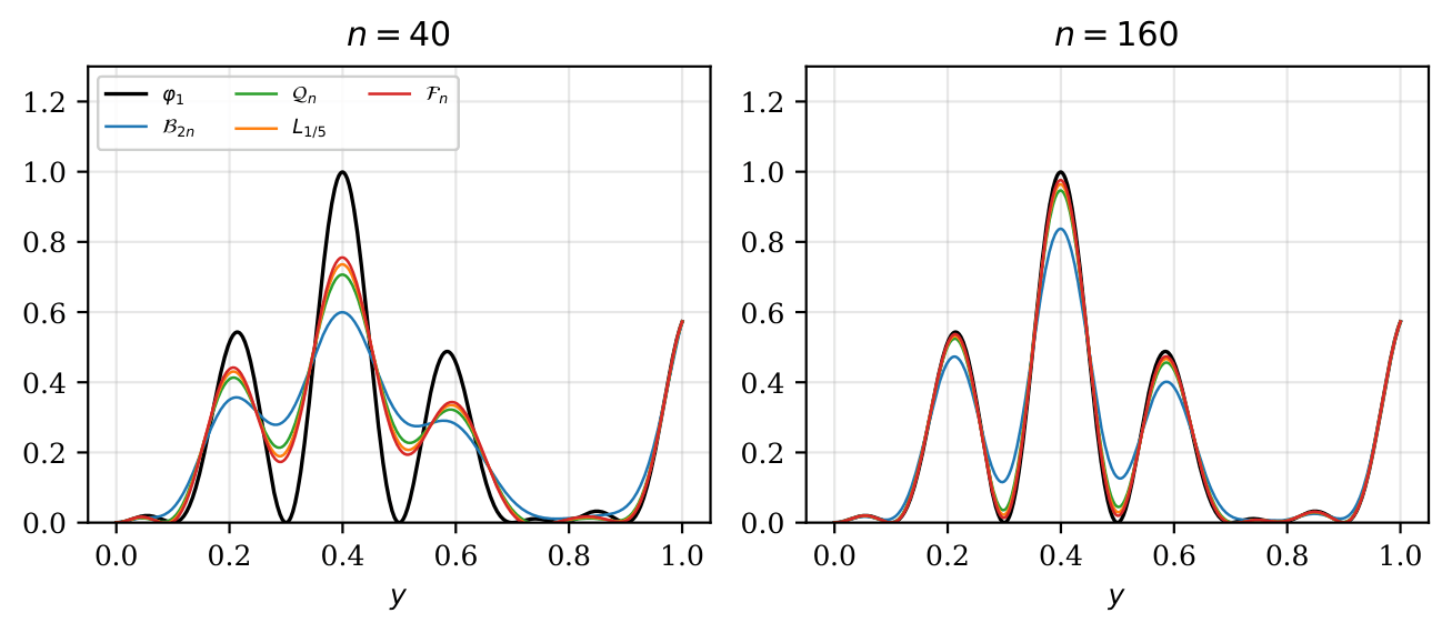
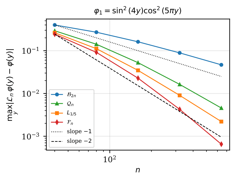
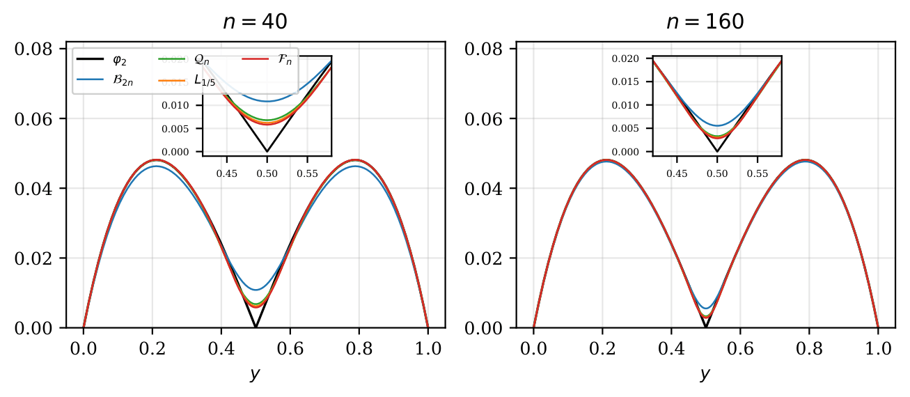
each entry being placed in the column of the finer $n$; the first column carries no entry, its predecessor not being tabulated. All values are given to three significant figures. Avg E is a grid average, that is a quadrature approximation to the $L^1$ error, and the EOC row refers to Max E alone. The two columns may therefore show different orders without disagreeing: in Table 2 the corner of ${\phi }_2$ contributes to the sup norm at every $n$ but occupies a shrinking set, so that Max E decays with order $\frac{1}{2}$ and Avg E with order $1$. The results are collected as follows. Tables 1 and 4 report the errors and the empirical orders for ${\phi }_1,\mathrm{\dots },{\phi }_4$ in turn. Figure 1 and Figure 3 show the four approximants for ${\phi }_1$ and ${\phi }_2$; for ${\phi }_3$ they would be indistinguishable from the function at this accuracy, so Figure 5 shows the pointwise errors instead, on a logarithmic vertical scale. Figures 2, 4, 6 and 7 show the maximum error against $n$ in logarithmic scales, the guide lines carrying the slopes predicted by the theory: $-1$ and $-2$ for the smooth functions, $-\frac{1}{2}$ for ${\phi }_2$.

The rapidly oscillating ${\phi }_1$ is the function on which ${ℱ}_n$ is at its best: its empirical order passes $2$ while that of ${ℬ}_{2n}$ is still below $1$. An order above $2$ is of course transient, all three combinations being of exact order $n^{-2}$ on ${\phi }_1\in C^{\mathrm{\infty }}$ by Theorem 6; it records that the asymptotic regime has not yet been reached, the quantity $n^2\mathrm{Max}E$ still decreasing towards its limit for ${ℱ}_n$ while it has nearly settled for ${𝒬}_n$. The member with the smaller asymptotic constant is the one that reaches its regime last, so that here a transient EOC above $2$ is itself a sign of the cancellation of the ${\phi }^{(4)}$ term.

	$n$	$40$	$80$	$160$	$320$	$640$
${ℬ}_{2n}$	Max E	$4.00\cdot {10}^{-1}$	$2.71\cdot {10}^{-1}$	$1.62\cdot {10}^{-1}$	$8.89\cdot {10}^{-2}$	$4.68\cdot {10}^{-2}$
	Avg E	$9.83\cdot {10}^{-2}$	$6.59\cdot {10}^{-2}$	$3.92\cdot {10}^{-2}$	$2.15\cdot {10}^{-2}$	$1.13\cdot {10}^{-2}$
	EOC	–	$0.56$	$0.74$	$0.86$	$0.93$
${𝒬}_n$	Max E	$2.92\cdot {10}^{-1}$	$1.42\cdot {10}^{-1}$	$5.25\cdot {10}^{-2}$	$1.63\cdot {10}^{-2}$	$4.57\cdot {10}^{-3}$
	Avg E	$7.38\cdot {10}^{-2}$	$3.55\cdot {10}^{-2}$	$1.31\cdot {10}^{-2}$	$4.06\cdot {10}^{-3}$	$1.14\cdot {10}^{-3}$
	EOC	–	$1.04$	$1.43$	$1.69$	$1.84$
$L_{1/5}$	Max E	$2.63\cdot {10}^{-1}$	$1.12\cdot {10}^{-1}$	$3.47\cdot {10}^{-2}$	$9.03\cdot {10}^{-3}$	$2.20\cdot {10}^{-3}$
	Avg E	$6.66\cdot {10}^{-2}$	$2.80\cdot {10}^{-2}$	$8.64\cdot {10}^{-3}$	$2.24\cdot {10}^{-3}$	$5.44\cdot {10}^{-4}$
	EOC	–	$1.24$	$1.69$	$1.94$	$2.04$
${ℱ}_n$	Max E	$2.43\cdot {10}^{-1}$	$9.17\cdot {10}^{-2}$	$2.28\cdot {10}^{-2}$	$4.25\cdot {10}^{-3}$	$6.52\cdot {10}^{-4}$
	Avg E	$6.20\cdot {10}^{-2}$	$2.33\cdot {10}^{-2}$	$5.75\cdot {10}^{-3}$	$1.04\cdot {10}^{-3}$	$1.55\cdot {10}^{-4}$
	EOC	–	$1.41$	$2.01$	$2.42$	$2.71$

Table 1. Errors and empirical orders for ${\phi }_1(y)={\sin }^2(4y){\cos }^2(5\pi y)$.

Figure 1. Approximation of ${\phi }_1$ by ${ℬ}_{2n}$, ${𝒬}_n$, $L_{1/5}$ and ${ℱ}_n$ at $n=\phantom{}$40, 160.

Figure 2. Maximum error against $n$ in logarithmic scales for ${\phi }_1$; the guide lines have slopes $-1$ and $-2$.

The corner of ${\phi }_2$ costs every operator its order: all four decay like $n{}^{-1/2}$ in the sup norm, and only a constant factor separates the three combinations.

	$n$	$40$	$80$	$160$	$320$	$640$
${ℬ}_{2n}$	Max E	$1.08\cdot {10}^{-2}$	$7.77\cdot {10}^{-3}$	$5.54\cdot {10}^{-3}$	$3.93\cdot {10}^{-3}$	$2.78\cdot {10}^{-3}$
	Avg E	$1.73\cdot {10}^{-3}$	$9.07\cdot {10}^{-4}$	$4.67\cdot {10}^{-4}$	$2.38\cdot {10}^{-4}$	$1.20\cdot {10}^{-4}$
	EOC	–	$0.48$	$0.49$	$0.49$	$0.50$
${𝒬}_n$	Max E	$6.79\cdot {10}^{-3}$	$4.71\cdot {10}^{-3}$	$3.30\cdot {10}^{-3}$	$2.32\cdot {10}^{-3}$	$1.64\cdot {10}^{-3}$
	Avg E	$4.45\cdot {10}^{-4}$	$2.20\cdot {10}^{-4}$	$1.09\cdot {10}^{-4}$	$5.46\cdot {10}^{-5}$	$2.73\cdot {10}^{-5}$
	EOC	–	$0.53$	$0.51$	$0.51$	$0.50$
$L_{1/5}$	Max E	$6.20\cdot {10}^{-3}$	$4.31\cdot {10}^{-3}$	$3.02\cdot {10}^{-3}$	$2.13\cdot {10}^{-3}$	$1.50\cdot {10}^{-3}$
	Avg E	$3.80\cdot {10}^{-4}$	$1.91\cdot {10}^{-4}$	$9.54\cdot {10}^{-5}$	$4.77\cdot {10}^{-5}$	$2.38\cdot {10}^{-5}$
	EOC	–	$0.53$	$0.51$	$0.51$	$0.50$
${ℱ}_n$	Max E	$5.81\cdot {10}^{-3}$	$4.04\cdot {10}^{-3}$	$2.84\cdot {10}^{-3}$	$2.00\cdot {10}^{-3}$	$1.41\cdot {10}^{-3}$
	Avg E	$3.79\cdot {10}^{-4}$	$1.88\cdot {10}^{-4}$	$9.30\cdot {10}^{-5}$	$4.62\cdot {10}^{-5}$	$2.30\cdot {10}^{-5}$
	EOC	–	$0.52$	$0.51$	$0.51$	$0.50$

Table 2. Errors and empirical orders for ${\phi }_2(y)=y(1-y)|y-\frac{1}{2}|$.

Figure 3. Approximation of ${\phi }_2$ by ${ℬ}_{2n}$, ${𝒬}_n$, $L_{1/5}$ and ${ℱ}_n$ at $n=\mathrm{40,160}$.

Figure 4. Maximum error against $n$ in logarithmic scales for ${\phi }_2$; the guide line has slope $-\frac{1}{2}$.

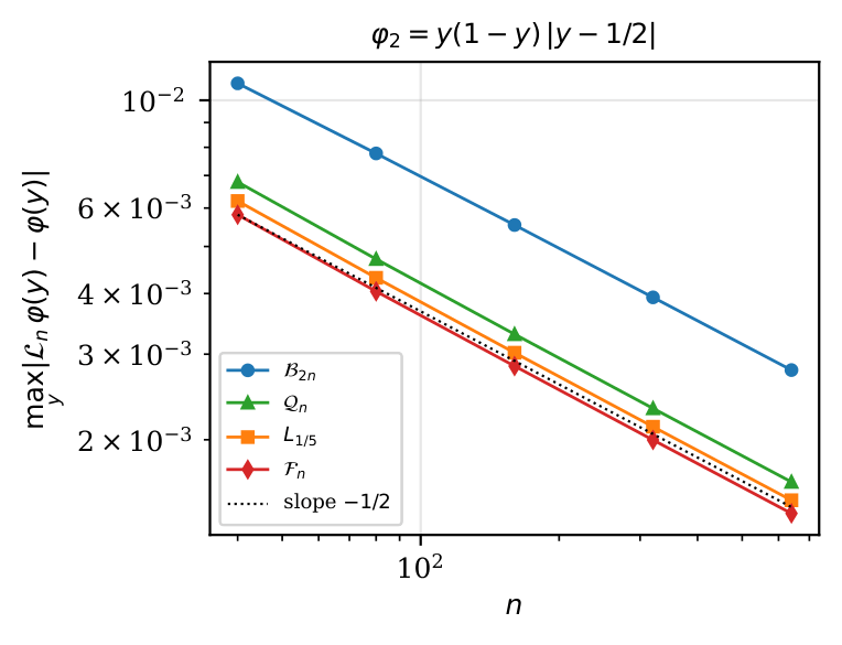
On the smooth ${\phi }_3$ the three combinations all reach the order $n^{-2}$, and their ranking is the reverse of the one on ${\phi }_1$.

	$n$	$40$	$80$	$160$	$320$	$640$
${ℬ}_{2n}$	Max E	$2.74\cdot {10}^{-3}$	$1.37\cdot {10}^{-3}$	$6.84\cdot {10}^{-4}$	$3.42\cdot {10}^{-4}$	$1.71\cdot {10}^{-4}$
	Avg E	$1.76\cdot {10}^{-3}$	$8.80\cdot {10}^{-4}$	$4.40\cdot {10}^{-4}$	$2.20\cdot {10}^{-4}$	$1.10\cdot {10}^{-4}$
	EOC	–	$1.00$	$1.00$	$1.00$	$1.00$
${𝒬}_n$	Max E	$9.39\cdot {10}^{-6}$	$2.35\cdot {10}^{-6}$	$5.87\cdot {10}^{-7}$	$1.47\cdot {10}^{-7}$	$3.67\cdot {10}^{-8}$
	Avg E	$5.63\cdot {10}^{-6}$	$1.41\cdot {10}^{-6}$	$3.52\cdot {10}^{-7}$	$8.80\cdot {10}^{-8}$	$2.20\cdot {10}^{-8}$
	EOC	–	$2.00$	$2.00$	$2.00$	$2.00$
$L_{1/5}$	Max E	$2.90\cdot {10}^{-5}$	$7.25\cdot {10}^{-6}$	$1.81\cdot {10}^{-6}$	$4.53\cdot {10}^{-7}$	$1.13\cdot {10}^{-7}$
	Avg E	$1.85\cdot {10}^{-5}$	$4.62\cdot {10}^{-6}$	$1.16\cdot {10}^{-6}$	$2.89\cdot {10}^{-7}$	$7.22\cdot {10}^{-8}$
	EOC	–	$2.00$	$2.00$	$2.00$	$2.00$
${ℱ}_n$	Max E	$4.98\cdot {10}^{-5}$	$1.25\cdot {10}^{-5}$	$3.13\cdot {10}^{-6}$	$7.82\cdot {10}^{-7}$	$1.96\cdot {10}^{-7}$
	Avg E	$3.04\cdot {10}^{-5}$	$7.58\cdot {10}^{-6}$	$1.90\cdot {10}^{-6}$	$4.74\cdot {10}^{-7}$	$1.18\cdot {10}^{-7}$
	EOC	–	$2.00$	$2.00$	$2.00$	$2.00$

Table 3. Errors and empirical orders for ${\phi }_3(y)=e^y$.

Figure 5. Pointwise absolute errors of ${ℬ}_{2n}$, ${𝒬}_n$, $L_{1/5}$ and ${ℱ}_n$ for ${\phi }_3$ at $n=160$, on a logarithmic vertical scale.

Figure 6. Maximum error against $n$ in logarithmic scales for ${\phi }_3$; the guide lines have slopes $-1$ and $-2$.

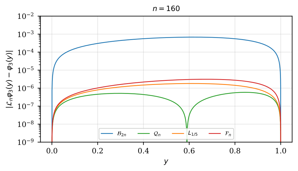
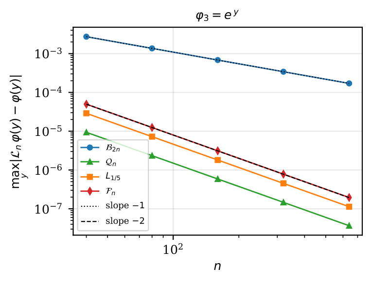
On ${\phi }_4$ the member selected by the third central moment, $L_{1/5}$, is the best of the three.

	$n$	$40$	$80$	$160$	$320$	$640$
${ℬ}_{2n}$	Max E	$1.53\cdot {10}^{-2}$	$7.68\cdot {10}^{-3}$	$3.85\cdot {10}^{-3}$	$1.93\cdot {10}^{-3}$	$9.63\cdot {10}^{-4}$
	Avg E	$7.94\cdot {10}^{-3}$	$3.97\cdot {10}^{-3}$	$1.99\cdot {10}^{-3}$	$9.94\cdot {10}^{-4}$	$4.97\cdot {10}^{-4}$
	EOC	–	$0.99$	$1.00$	$1.00$	$1.00$
${𝒬}_n$	Max E	$2.28\cdot {10}^{-4}$	$5.83\cdot {10}^{-5}$	$1.47\cdot {10}^{-5}$	$3.70\cdot {10}^{-6}$	$9.27\cdot {10}^{-7}$
	Avg E	$1.03\cdot {10}^{-4}$	$2.62\cdot {10}^{-5}$	$6.60\cdot {10}^{-6}$	$1.66\cdot {10}^{-6}$	$4.15\cdot {10}^{-7}$
	EOC	–	$1.97$	$1.99$	$1.99$	$2.00$
$L_{1/5}$	Max E	$4.98\cdot {10}^{-5}$	$1.28\cdot {10}^{-5}$	$3.39\cdot {10}^{-6}$	$8.85\cdot {10}^{-7}$	$2.26\cdot {10}^{-7}$
	Avg E	$3.66\cdot {10}^{-5}$	$9.21\cdot {10}^{-6}$	$2.31\cdot {10}^{-6}$	$5.80\cdot {10}^{-7}$	$1.45\cdot {10}^{-7}$
	EOC	–	$1.96$	$1.92$	$1.94$	$1.97$
${ℱ}_n$	Max E	$2.21\cdot {10}^{-4}$	$5.96\cdot {10}^{-5}$	$1.55\cdot {10}^{-5}$	$3.94\cdot {10}^{-6}$	$9.94\cdot {10}^{-7}$
	Avg E	$9.70\cdot {10}^{-5}$	$2.55\cdot {10}^{-5}$	$6.56\cdot {10}^{-6}$	$1.66\cdot {10}^{-6}$	$4.19\cdot {10}^{-7}$
	EOC	–	$1.89$	$1.95$	$1.97$	$1.99$

Table 4. Errors and empirical orders for ${\phi }_4(y)=\sin (\pi y)$.

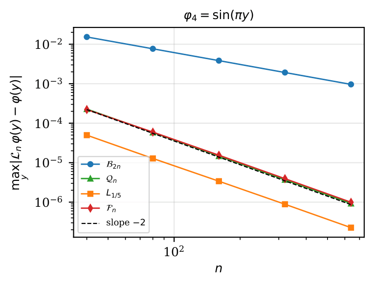
Maximum error against $n$ in logarithmic scales for ${\phi }_4$; the guide line has slope $-2$

Figure 7. Maximum error for ${\phi }_4$.

${ℱ}_n$ is the most accurate of the three combinations in Tables 1 and 2 and the least accurate in Table 3, and Section 3 says why. On ${\phi }_1$, whose fourth derivative is large relative to its second, the first difference decides and ${ℱ}_n$ wins; on ${\phi }_3$, whose derivatives are of comparable size, the second decides and ${𝒬}_n$ wins. The observed factors are the predicted ones: the ratios $4.98\cdot {10}^{-5}/9.39\cdot {10}^{-6}=5.30$ and $2.90\cdot {10}^{-5}/9.39\cdot {10}^{-6}=3.09$ of Table 3 agree with the ratios $5.33$ and $3.08$ of the corresponding asymptotic constants of (8). The formula itself is confirmed at three values of $c$ at once: on ${\phi }_4$, $n^2\mathrm{Max}E$ at $n=640$ equals $0.380$, $0.093$ and $0.407$ for ${𝒬}_n$, $L_{1/5}$ and ${ℱ}_n$, against $0.381$, $0.095$ and $0.411$ for ${\max }_y$ of the modulus of the constant that (8) gives at $c=0$, $c=\frac{1}{5}$ and $c=\frac{1}{3}$, the deviation falling like $n^{-1}$. On ${\phi }_2$ no operator reaches the order $n^{-2}$, the missing smoothness leaving only a constant factor between them.

Nor is ${ℱ}_n$ the best member of (3) on every function: on ${\phi }_4$ the member selected by the third central moment, $L_{1/5}$, is about four times more accurate than either of the other two, the ${\phi }^{\prime \prime \prime }$ term being the one that dominates there. Which member is best adapted to a given function is read off from (8), and it is ${ℱ}_n$ precisely when ${\phi }^{(4)}$ dominates.

5. Conclusion

The family (3) is what the two requirements – preservation of constants and the vanishing of the $𝒪(n^{-1})$ term of the second central moment – leave free. Every member has approximation order $𝒪(n^{-2})$, an order already available from Butzer’s operator ${𝒬}_n=L_0$, so the order itself is not what the construction contributes; what the remaining free parameter can still do is annihilate the leading term of exactly one of the three central moments that enter the error at that order, and this classifies the distinguished members of the family as $L_0={𝒬}_n$, $L_{1/5}$ and $L_{1/3}={ℱ}_n$, the first classical and the other two new. For the third we proved a uniform bound, direct estimates of order $o(n^{-1})$ for $\phi \in C^2[0,1]$ and $n^{-2}$ for $\phi \in C^4[0,1]$ with explicit constants, a refinement of the latter in which the contribution of ${\phi }^{(4)}$ is $o(n^{-2})$, an estimate in a modified fourth-order $K$-functional, uniform convergence on $C[0,1]$, and the Voronovskaja-type formula of Theorem 6, stated for the whole family.

That formula is not the only place where the members differ, but almost: the estimates of Theorems 1, 2, 3 and 5 hold for ${𝒬}_n$ as well, with comparable or better constants, and the sole quantitative exception is Theorem 4, whose $o(n^{-2})$ gain rests on the cancellation ${\mathrm{\Omega }}_{n,4}=𝒪(n^{-3})$ and has no counterpart for ${𝒬}_n$. No member is positive either, so that the shape-preserving properties of ${ℬ}_n$ are lost in every case. No member is uniformly better than the others either, and which one is best adapted to a given function is read off from the three coefficients of (8) – it is ${ℱ}_n$ precisely when ${\phi }^{(4)}$ dominates – as the experiments of Section 4 confirm, each of the three being the most accurate on at least one of the four test functions. Two directions seem worth pursuing. The members singled out by the higher central moments through Section 2 begin at $m=5$ and have not been examined here, nor has the description of the classes of functions on which each distinguished member is preferable, of which Section 4 gives only numerical evidence. The second is the extension of the same selection principle to bivariate operators on multidimensional domains, and to families carrying shape parameters, where an additional degree of freedom would allow more than one moment to be annihilated at once.

References

- [1] A.M. Acu and I. Raşa, Ulam stability for the composition of operators, Symmetry, 12 (2020) no. 7, Art. no. 1159. https://doi.org/10.3390/sym12071159
- [2] F. Altomare and M. Campiti, Korovkin-type Approximation Theory and its Applications, de Gruyter Studies in Mathematics 17, Walter de Gruyter, Berlin, 1994. https://doi.org/10.1515/9783110884586
- [3] S.N. Bernstein, Démonstration du Théorème de Weierstrass fondée sur le calcul des probabilités, Commun. Soc. Math. Kharkov, 13 (1912) no. 1, pp. 1–2.
- [4] P.L. Butzer, Linear combinations of Bernstein polynomials, Canad. J. Math., 5 (1953), pp. 559–567. https://doi.org/10.4153/CJM-1953-063-7
- [5] R.A. DeVore and G.G. Lorentz, Constructive Approximation, Grundlehren der mathematischen Wissenschaften 303, Springer-Verlag, Berlin, 1993.
- [6] Z. Ditzian and K.G. Ivanov, Strong converse inequalities, J. Anal. Math., 61 (1993), pp. 61–111. https://doi.org/10.1007/BF02788839
- [7] Z. Ditzian and V. Totik, Moduli of Smoothness, Springer Series in Computational Mathematics 9, Springer-Verlag, New York, 1987. https://doi.org/10.1007/978-1-4612-4778-4
- [8] I. Gavrea and M. Ivan, Asymptotic behaviour of the iterates of positive linear operators, Abstract and Applied Analysis, 2011 (2011), Art. ID 670509. https://doi.org/10.1155/2011/670509
- [9] H. Gonska, On the degree of approximation in Voronovskaja’s theorem, Studia Univ. Babeş-Bolyai Math., 52 (2007) no. 3, pp. 103–115.
- [10] A. Kajla and T. Acar, Modified -Bernstein operators with better approximation properties, Ann. Funct. Anal., 10 (2019) no. 4, pp. 570–582. https://doi.org/10.1215/20088752-2019-0015
- [11] R.P. Kelisky and T.J. Rivlin, Iterates of Bernstein polynomials, Pacific J. Math., 21 (1967) no. 3, pp. 511–520. https://doi.org/10.2140/pjm.1967.21.511
- [12] J.P. King, Positive linear operators which preserve , Acta Math. Hungar., 99 (2003) no. 3, pp. 203–208. https://doi.org/10.1023/A:1024571126455
- [13] G.G. Lorentz, Bernstein Polynomials, University of Toronto Press, Toronto, 1953.
- [14] C.P. May, Saturation and inverse theorems for combinations of a class of exponential-type operators, Canad. J. Math., 28 (1976) no. 6, pp. 1224–1250. https://doi.org/10.4153/CJM-1976-123-8
- [15] C.A. Micchelli, The saturation class and iterates of the Bernstein polynomials, J. Approx. Theory, 8 (1973) no. 1, pp. 1–18. https://doi.org/10.1016/0021-9045(73)90028-2
- [16] F. Özger, H.M. Srivastava and S.A. Mohiuddine, Approximation of functions by a new class of generalized Bernstein-Schurer operators, RACSAM, 114 (2020) no. 4, Art. no. 173. https://doi.org/10.1007/s13398-020-00903-6
- [17] R.S. Rajawat, K.K. Singh and V.N. Mishra, Approximation by modified Bernstein polynomials based on real parameters, Math. Found. Comput., 7 (2024) no. 3, pp. 297–309. https://doi.org/10.3934/mfc.2023005
- [18] I. Raşa, Iterated Boolean sums of Bernstein and related operators, Rev. Anal. Numér. Théor. Approx., 35 (2006) no. 1, pp. 111–115. https://doi.org/10.33993/jnaat351-1018
- [19] W. Rudin, Principles of Mathematical Analysis, 3rd ed., McGraw–Hill, New York, 1976.
- [20] P. Sablonnière, Bernstein quasi-interpolants, Approx. Theory Appl., 8 (1992) no. 3, pp. 62–76.
- [21] M. Sofyalıoğlu, K. Kanat and B. Çekim, Parametric Generalization of the Modified Bernstein Operators, Filomat, 36 (2022) no. 5, pp. 1699–1709. https://doi.org/10.2298/FIL2205699S
- [22] F. Usta, On New Modification of Bernstein Operators: Theory and Applications, Iran. J. Sci. Technol. Trans. Sci., 44 (2020) no. 6, pp. 1801–1809. https://doi.org/10.1007/s40995-020-00919-y
- [23] G. Zhou and Q.-B. Cai, Approximation properties of -Bernstein operators, Filomat, 39 (2025) no. 23, pp. 8193–8207. https://doi.org/10.2298/FIL2523193Z