A comparative study of Filon-type rules
for oscillatory integrals

Hassan Majidian¹

(Date: December 18, 2023; accepted: February 22, 2024; published online: March 6, 2024.)

Abstract.

Our aim is to answer the following question: “Among the Filon-type methods for computing oscillatory integrals, which one is the most efficient in practice?”. We first discuss why we should seek the answer among the family of Filon-Clenshaw-Curtis rules. A theoretical analysis accompanied by a set of numerical experiments reveals that the plain Filon-Clenshaw-Curtis rules reach a given accuracy faster than the (adaptive) extended Filon-Clenshaw-Curtis rules. The comparison is based on the CPU run-time for certain wave numbers (medium and large).

Key words and phrases:

oscillatory integral, Filon-Clenshaw-Curtis rule, extended FCC rule, adaptive FCC+ rule.

2005 Mathematics Subject Classification:

65D32, 65Y20

¹Department of Multidisciplinary Studies, Faculty of Encyclopedia Studies, Institute for Humanities and Cultural Studies, PO Box 14155-6419, Tehran, Iran, e-mail: h.majidian@ihcs.ac.ir.

1. Introduction

Consider the oscillatory integral

(1)

I_{k}(f):=\int_{-1}^{1}f(x)\mathrm{e}^{\mathrm{i}kx}\,\mathrm{d}x,

where $f$ is a given smooth function on $[-1,1]$ , and the wave number ${k>0}$ is rather large. Filon-type methods, in brief, reads as $I_{k}(p)$ , where $p$ is a polynomial approximation of $f$ in $[-1,1]$ . In details, the interpolation polynomial $p$ is generally expanded as

(2)

p(x)=\sum_{j}\alpha_{j}q_{j}(x),\quad x\in[-1,1],

where $q_{j}$ is a polynomial of order $j$ for each $j$ . The scalars $\alpha_{j}$ , for all $j$ , are computed in the construction phase of $p$ . Thus, the Filon-type method is expanded as

(3)

I_{k}(p)=\sum_{j}\alpha_{j}m_{j},

where ${m_{j}:=I_{k}(q_{j})}$ are the moments to be evaluated.

Certainly, accuracy of a Filon-type method is proportional to the accuracy of the corresponding polynomial approximation because

(4)

\left|I_{k}(f)-I_{k}(p)\right|<2\|f-p\|_{\infty}.

In practice, what is the best choice of $p$ of a given degree? Even if we restrict our investigation to interpolation, there are a tremendous number of interpolation polynomials approximating a smooth function satisfactory, e.g. splines, Hermite-Birkhoff interpolation, and those based on orthogonal polynomials and their roots or extrema. The main question motivating this research is, which interpolation is the best choice for Filon-type methods? Beside the accuracy of the interpolation polynomial $p$ on $[-1,1]$ , there are mainly three other aspects that affect the efficiency of the Filon-type method $I_{k}(p)$ in practice: (i) the cost of construction of $p$ , (ii) the cost of computing the moments, (iii) and the order of interpolation at the endpoints $\pm 1$ .

In general, Lagrange interpolation at arbitrary points is rather costly. However, in [6], a rapid and stable construction method is proposed based on the fast multipole method (FMM) of [8]. Instead of an arbitrary set of interpolation points, however, one prefers roots or extrema of orthogonal polynomials and utilize FFT for better performance. Among several kinds of orthogonal polynomials, Chebyshev polynomials are often used mainly because their roots and extrema are in the most simple and explicit forms.

For fast computing the moments, one prefers polynomials which satisfy a recurrence relation. Then the moments can be computed recursively with few computational cost. Orthogonal polynomials not only can be constructed efficiently by FFT, but also they satisfy three-term recurrence relations. Assume that $(q_{j})$ in (2) satisfies the three-term recurrence relation

(5)

q_{j+2}=a_{j}q_{j+1}+b_{j}q_{j},\qquad j=0,1,\ldots,

where $a_{j}$ and $b_{j}$ are known scalars with ${|a_{j}|+|b_{j}|\neq 0}$ for all $j$ . The first two moments can easily be computed analytically. Then, the other ones are computed by (5), recursively:

(6)

m_{j+2}=a_{j}m_{j+1}+b_{j}m_{j},\qquad j=0,1,\ldots.

On the other hand, the asymptotic expansion of the oscillatory integral $I_{k}(f)$ turns out that the value of $I_{k}(f)$ is mostly determined by its amplitude, $f$ , and their derivatives up to some order at the endpoints $\pm 1$ . More precisely, if $f$ is smooth enough in ${[-1,1]}$ , and

(7)

\left(f^{(m)}-p^{(m)}\right)(\pm 1)=0,\qquad m=0,\ldots,s,

for some integer ${s\geq 0}$ , then

(8)

\left|I_{k}(f)-I_{k}(p)\right|=\mathcal{O}(k^{-s-2}),\quad\text{as }{k\to\infty}

(see, e.g., [11]). Therefore, not only the accuracy of the interpolation, i.e. ${\|f-p\|_{\infty}}$ , is important for the total accuracy of a Filon-type rule $I_{k}(p)$ , but also its order $s$ at the endpoints.

The conditions (7) implies an example of Hermite-Birkhoff interpolation, which construction rarely utilizes fast algorithms like FFT or FMM. Interpolation at the Clenshaw-Curtis points ${t_{n,N}:=\cos(n\pi/N)}$ , ${j=0,\ldots,n}$ , have all the above advantages. Because of the distribution of the Clenshaw-Curtis points in $[-1,1]$ , interpolation at them is most accurate and numerically stable. Moreover, thanks to the three-term recurrence relation for the Chebyshev polynomials, it can stably be constructed by FFT at the cost of $\mathcal{O}(n\log n)$ (see [5]). In addition, the computational cost for computing $t_{n}$ , ${n=0,\ldots,N}$ , is negligible. Finally, having the Lagrange interpolant at the Clenshaw-Curtis, one can efficiently construct the corresponding Hermite-Birkhoff interpolant $p$ that satisfies (7), too (see [15]).

Therefore, without doubt, Filon-Clenshaw-Curtis (FCC) rules and their extensions are the most efficient Filon-type rules for computing the oscillatory integral (1). Extended FCC (FCC+) rules and their adaptive versions can be constructed efficiently by the algorithms of [15] and [14], respectively. To the best of our knowledge, they are the most efficient algorithms for constructing the FCC+ and adaptive FCC+ rules so far.

In comparison with the algorithm of [5] for constructing the FCC rules, the algorithms of [15] and [14] are more complex. This difference in the computational costs may be negligible when the maximum order of derivatives $s$ in the FCC+ rules is rather small. On the other hand, the asymptotic order of an (adaptive) FCC+ rule is better than that of the corresponding FCC rule. Actually, one cannot readily answer which algorithm is more efficient, and this question naturally triggers a comparative study. Indeed, this paper fills a gap in the literature and help in the comparison between Filon-type methods.

In this paper, we carry out a set of numerical experiments to compare efficiency of FCC, FFC+, and adaptive FCC+. Actually, we are interested in the CPU run-time to achieve a specific accuracy. We apply these three classes of rules to a set of oscillatory integrals with different regularity characteristics. Since FCC is less complex than the other rules, one can use more interpolation points for the same computational effort as (adaptive) FCC+.

The rest of the paper is organized as follows. In Section 2, we carry out a set of numerical experiments in order to compare the efficiency of the FCC and the FCC+ rules. In Section 3, the same is done for the FCC and the adaptive FCC+ rules. We also modify Theorem 2.2 of [14] and give a more practical error bound for the adaptive FCC+ rules that is explicit in $k$ and the rule parameters. In Section 4, we account several other advantages of the FCC rules over the (adaptive) FCC+ ones. Finally, we bring some conclusions in Section 5.

2. FCC vs FCC+

In this section, we compare the efficiency of the FCC and FCC+ rules. In contrast to the common ideas in the literature, we see that the FCC+ rules have no advantages over the plain FCC rules in practice. At first, we give a brief review of the FCC+ rules (see [7, 15]).

2.1. A review of the FCC+ rules

The ( ${N+1}$ )-point FCC+ rule of order ${s\geq 1}$ is defined by

(9)

I^{\mathrm{FCC+}}_{k,N,s}(f):=I_{k}(p_{N+2s}),

where $p_{N+2s}$ is the ${(N+2s)^{\mathrm{th}}}$ degree Hermite interpolation polynomial satisfying the following interpolation conditions (see [15]):


(10a)	$\displaystyle p_{N+2s}(t_{n,N})$	$\displaystyle=f(t_{n,N}),\quad n=0,\ldots,N,$
(10b)	$\displaystyle p_{N+2s}^{(m)}(\pm 1)$	$\displaystyle=f^{(m)}(\pm 1),\quad m=1,\ldots,s.$

Then, the asymptotic error of the rule will be

(11)

\left|I_{k}(f)-I^{\mathrm{FCC+}}_{k,N,s}(f)\right|=\mathcal{O}\left(k^{-s-2}%\right),

see, e.g., [11].

An important advantage of the FCC rules over the FCC+ ones is that there are error estimates for the FCC rules, which are applicable even if $f$ is of confined regularity. Furthermore, they are explicit in both $k$ and $N$ (see [4, 5, 20, 21]). Such error bounds do not exist for the FCC+ rules so far (see [15] for details).

In [7], an efficient algorithm is proposed for constructing the FCC+ rule (9) that can be implemented by $\mathcal{O}\left(N\log N+s^{3}\right)$ flops. A more efficient algorithm was later proposed in [15]. One advantage of the latter is that its computational cost can be determined precisely. By the algorithm of [15], one needs $\mathcal{O}(s^{3}+Ns+s^{2})$ flops to extend the ( ${N+1}$ )-point FCC rule to the corresponding FCC+ rule of order $s$ in a natural way. Thus, beside its simplicity and naturality, the algorithm of [15] enables one to compare computational costs of the two rules easily. The algorithm for constructing the ( ${N+1}$ )-point FCC+ rule of order ${s>1}$ leads to two linear systems of order $s$ . However, the FCC+ rules of order 1 can be stated explicitly, and one only needs about ${3N+14}$ extra flops to build it from the corresponding ( ${N+1}$ )-point FCC rule.

2.2. The race for convergence speed

Error estimate (11) turns out that for a fixed $N$ , the asymptotic decaying rate of the error of $I^{\mathrm{FCC+}}_{k,N,s}(f)$ is higher than that of $I^{\mathrm{FCC}}_{k,N}(f)$ , and it grows by $s$ . On the other hand for rather large $N$ , the complexity of the FCC rule, $\mathcal{O}\left(N\log N\right)$ , is comparable to that of the FCC+ rule, $\mathcal{O}\left(N\log N+s^{3}\right)$ because $s$ is usually taken rather small in practice. Thus, some authors conclude that the FCC+ rules are always the winner in the competition with the FCC rules. According to [3],“the generalization of FCC … enjoys all the advantages of ‘plain’ FCC … in cost and simplicity, while arbitrarily increasing the asymptotic rate of decay of the error” (p. 66).

In this section, we show that such claims are in doubt in practice. Although, it may be required in some applications to compute $I_{k}(f)$ for several $k$ and $f$ , but each time, we face the problem of computing one integral with a fixed parameter $k$ and a fixed amplitude function $f$ . The FCC+ rule $I^{\mathrm{FCC+}}_{k,N_{1},s}(f)$ approximates the integral to a specific accuracy for some rather large integers $N_{1}$ and $s$ . As mentioned above, the FCC rule $I^{\mathrm{FCC}}_{k,N_{1}}(f)$ with the same $N_{1}$ generally achieves less accuracy. However, we may choose larger integer ${N_{2}>N_{1}}$ and achieve the same accuracy or even better while the computational cost does not exceed that of $I^{\mathrm{FCC+}}_{k,N_{1},s}(f)$ . Recall from [15] that the FCC+ rule $I^{\mathrm{FCC+}}_{k,N,s}(f)$ is more complex than its corresponding FCC rule $I^{\mathrm{FCC}}_{k,N}(f)$ by at least ${\mathcal{O}(s^{3})+N(8s-5)+s(17s+9)+1}$ flops. Now assume that $C_{k}(N)$ is the exact number of flops for constructing $I^{\mathrm{FCC}}_{k,N}(f)$ by the algorithm proposed in [5]. Thus, in order to compare the simplicity of the two rules $I^{\mathrm{FCC+}}_{k,N_{1},s}(f)$ and $I^{\mathrm{FCC}}_{k,N_{2}}(f)$ , we should compare the two numbers $C_{k}(N_{2})$ and

C_{k}(N_{1})+\mathcal{O}(s^{3})+N_{1}(8s-5)+s(17s+9)+1.

Even if we compute the number of flops for construction of the two rules exactly, error estimates (specially for the FCC+ rules) are not so sharp that the accuracy of the rules can be estimated a priori for a given $N$ and $s$ . For practical examining the efficiency of an approximation method (or rule), one can consider the run-time that the method consumes in a specific machine to reach a given accuracy.

Refer to caption — Figure 1. Accuracy vs execution time (in miliseconds) when the FCC rules and the FCC+ rules with $s=1,2,3$ are applied to $I_{k}(f)$ for $f(x)=(1+x)/(1+x^{2})$ and some wave numbers $k$ that range from small to quite large values.

In the following, we apply FCC and FCC+ to a set of oscillatory integrals (1), covering wave numbers from moderate to quite large values. We try to have at least one sample of the amplitude function in each class of $C^{\infty}([-1,1])$ , $C^{m}([-1,1])$ for some integer ${m>0}$ , elementary functions, and non-elementary functions. In each method, we choose $N$ as the minimum number of interpolation points to achieve a given accuracy. As discussed above, this number for FCC is generally larger than that of FCC+.

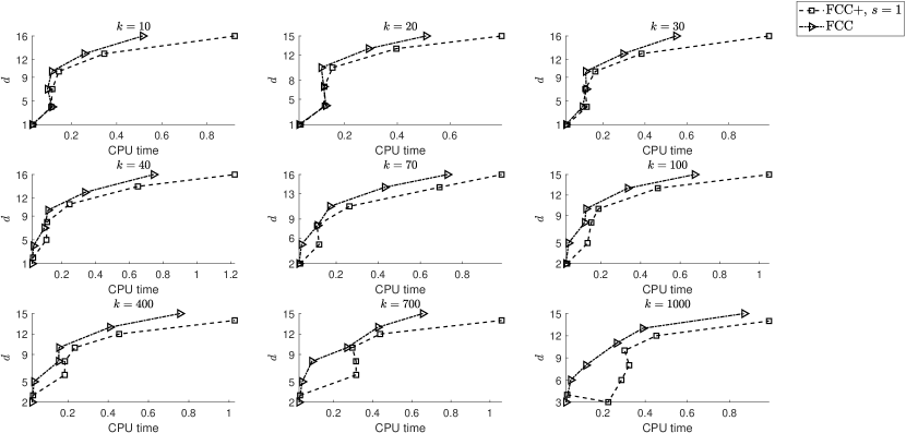
Experiment 1.

Let ${d:=-\log_{10}E}$ , where $E$ is the relative error of an approximation. Indeed, $d$ is roughly the number of correct significant digits in the approximation. In Fig. 1, we plotted $d$ versus the machine run-time (in milliseconds) for the FCC and FCC+ rules (9) of orders ${s=1,2,3}$ when applied to $I_{k}(f)$ with ${f(x)=(1+x)/(1+x^{2})}$ and some wave numbers ${k>0}$ ranging from small to quite large values. Note that each time an algorithm is run by a specific machine, the run-time may vary a little mainly because of invisible services running in the background on the operating system (OS). For that reason, in all the numerical experiments in the sequel concerning run-times, we run the corresponding Matlab algorithm ten times and consider the minimum of the run-times. For ${k\geq 70}$ , for which the plots have space enough, we label each marker by the corresponding $N$ . All the Matlab codes have been optimized in order to use less memory and take less time to execute.

Although, the derivatives of $f$ have been precalculated manually to the advantage of FCC+, our numerical experiments turn out that FCC are still more efficient than FCC+, especially for moderate and larger $k$ . Also, among the FCC+ rules, those with smaller $s$ are more efficient. This observation is against some authors’ claims that the FCC+ rules are ‘the winner’ just because the asymptotic decaying rates of their error are higher than those of the FCC rules. As it is seen, for a specific $N$ , accuracy of the FCC+ rules is higher than that of the FCC rule, and this accuracy enhances as $s$ grows. For example, in the last plot corresponding to ${k=1000}$ , the 31-point FCC rule, the 26-point FCC+ rule of order 1, the 19-point FCC+ rule of order 2, and the 12-point FCC+ rule of order 3 reach approximately 13 correct significant digits. However, the FCC rules ultimately reach a given accuracy faster than all the FCC+ rules.

Experiment 2.

The amplitude function $f$ in the previous experiment is infinitely differentiable. Here, we consider $f(x)=x^{3/2}$ , $x\in[0,1]$ , for which only the first derivative exists on $[0,1]$ . Thus, the parameter $s$ in the FCC+ rules cannot exceed 1. In Fig. 2, we have plotted the accuracy $d$ versus the machine run-time (in milliseconds) for the FCC rules and the FCC+ rules of order 1. Because in this example the degree of regularity is low, the rules reach a given accuracy only for larger $N$ .

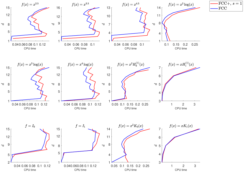
Experiment 3.

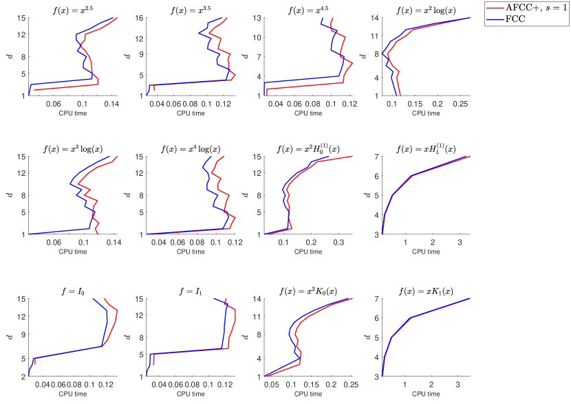
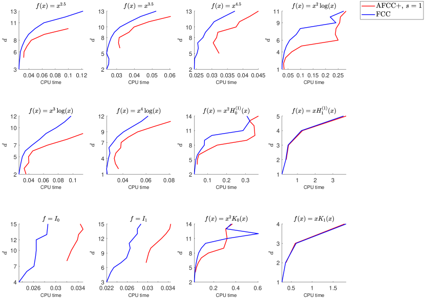
In order to see if the above experimental results hold for other amplitude functions $f$ , here we choose a set of elementary and non-elementary functions of various types on $[0,1]$ :

\begin{array}[]{cl}x^{\alpha},&\alpha=2.5,3.5,4.5,\\[2.15277pt]x^{n}\log(x),&n=2,3,4,\\[2.15277pt]x^{2}H^{(1)}_{0}(x),&xH^{(1)}_{1}(x),\\[2.15277pt]I_{\nu}(x),&\nu=0,1,\\[2.15277pt]x^{2}K_{0}(x),&xK_{1}(x).\\[2.15277pt]\end{array}

Here, $H^{(1)}_{\nu}$ , $I_{\nu}$ , and $K_{\nu}$ are the Hankel function of the first kind, the modified Bessel function of the first kind, and the modified Bessel function of the second kind of order $\nu$ , respectively. $I_{\nu}(x)$ is smooth on $[0,1]$ while each of the other functions has one and only one singularity at zero. The singularity is bounded and of algebraic or logarithmic type.

In Fig. 3 and Fig. 4, we have compared the efficiency of the FCC rules and FCC+ rules of order one for computing $I_{10}(f)$ and $I_{1000}(f)$ , respectively. As it is seen, the FCC rules are most often the winner, especially for the larger wave number.

3. FCC vs Adaptive FCC+

In this section, we compare the efficiency in practice of the FCC and the adaptive FCC+ rules of [14]. An adaptive FCC+ rule and its corresponding FCC+ rule always have the same asymptotic order while the former is derivative-free and less complex. We will see, however, that in the race to achieve a given accuracy, the adaptive FCC+ rules are still overtaken by the corresponding FCC rules. At first, we give a brief review of [14], where the concept of adaptive FCC+ rules has been introduced for the first time.

3.1. A review of the adaptive FCC+ rules

The ( ${N+2s+1}$ )-point adaptive FCC+ rule of order $s$ is defined by

(12)

I^{\mathrm{AFCC+}}_{k,N,s}(f):=I_{k}(p_{N+2s}),

where ${p_{N+2s}}$ is the Lagrange interpolant of $f$ at $t_{n,N}$ , for ${n=0,\ldots,N}$ , and $2s$ extra points $t^{\prime}_{m}(k)$ , $t^{\prime\prime}_{m}(k)$ , ${m=1,\ldots,s}$ , that should be near the endpoints $\pm 1$ and are defined as follows:

(13)

t^{\prime}_{m}(k):=\cos(\eta_{m}(k))\quad\mbox{with}\quad\eta_{m}(k):=\sqrt{%\frac{m}{k+1}},\quad t^{\prime\prime}_{m}(k):=-t^{\prime}_{m}(k).

As mentioned above, an adaptive FCC+ rule preserves the asymptotic order of the corresponding FCC+ rule. More precisely, we have the following result proved in [14]:

Theorem 1.

Assume that ${f\in C^{N+2s+1}([-1,1])}$ . Then,

(14)

\left|I_{k}(f)-I^{\mathrm{AFCC+}}_{k,N,s}(f)\right|=\mathcal{O}\left(k^{-s-2}%\right),

as $k\to\infty$ .

In contrast to the FCC+ rules, there are error bounds for the adaptive FCC+ rules that are explicit in all the three parameters $k$ , $N$ , and $s$ .

Corollary 2.

Assume that ${f\in C^{N+2s+1}([-1,1])}$ , and ${k+1\geq 2s}$ . Then,

(15)

\left|I^{\mathrm{AFCC+}}_{k,N,s}(f)-I_{k}(f)\right|\leq k^{-2}2^{-N}\,\tfrac{1%7}{(N+2s-4)!}\left\|f^{(N+2s+1)}\right\|_{\infty},

for all ${N>1}$ .

Proof.

For ${N>1}$ ,

	$\displaystyle\tfrac{2Ns!\,k^{-s}}{(N+2s+1)!}+\tfrac{\gamma_{N,s}}{(N+2s-1)!}$	$\displaystyle<\tfrac{2}{(N+2s-4)!}\left(N^{-4}k^{-s}s!+2\right)$
		$\displaystyle<\tfrac{2(1/8+2)}{(N+2s-4)!},$

where ${\gamma_{N,s}:=s(4N+2s-1)+N(2N^{2}+1)/3}$ . Now, the result is followed by Theorem 2.2 of [14]. $\qquad\blacksquare$

In [14], it was shown numerically that, adaptive FCC+ is always more efficient than FCC+. However, our numerical experiments in the next section show that it is still overtaken by FCC is the race to achieve a given accuracy.

3.2. The race for convergence speed

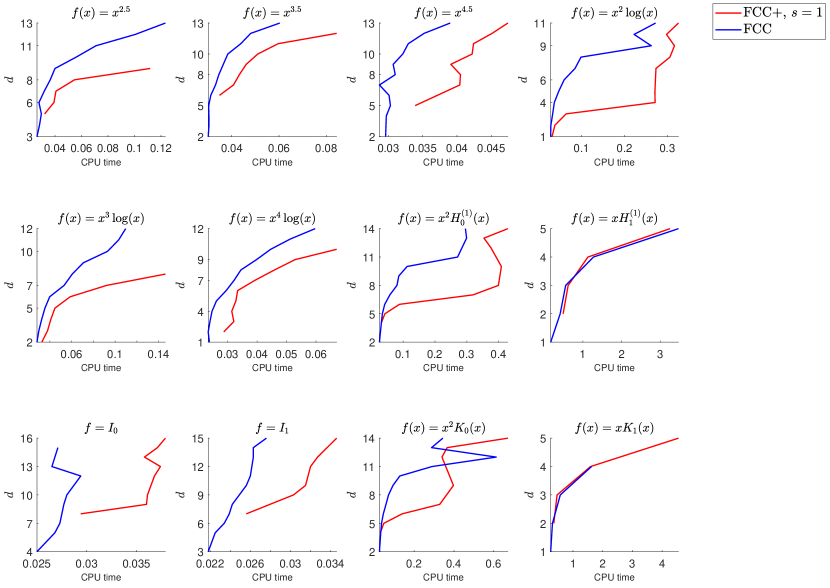
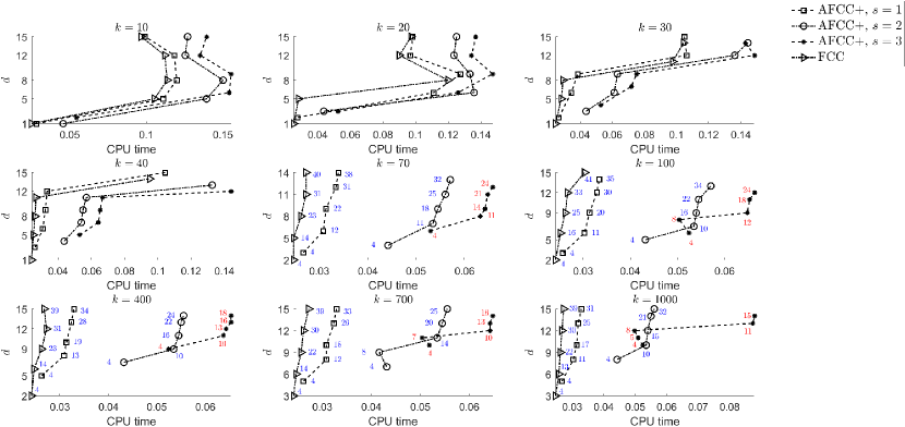
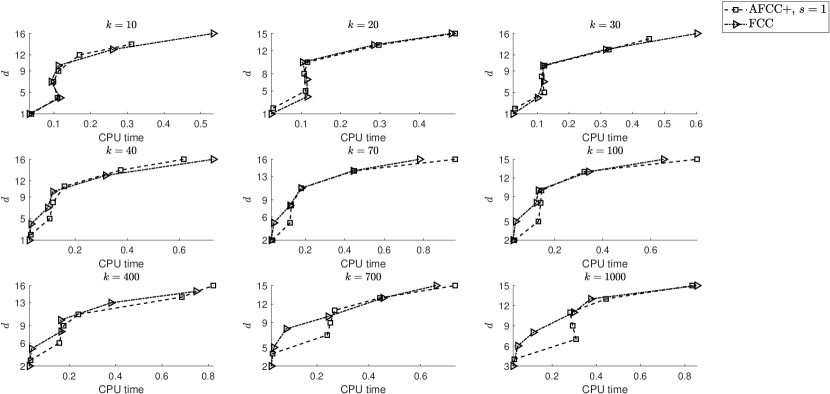
In this section, we repeat the numerical experiments of Section 2.2, now by the adaptive FCC+ instead of the FCC+ rules. The same discussion is applicable here, too. In Fig. 5–Fig. 8, we compare convergence rates of the adaptive FCC+ rules and the corresponding FCC rules. The results are the same as in Fig. 1–Fig. 4, and FCC is always the winner.

4. Other advantages of FCC rules

The FCC rules have further advantages over the FCC+ and adaptive FCC+ rules. In this section, we account some of them.

(1)

Composite FCC rules can readily be developed [4] while the composite versions of the (adaptive) FCC+ rules require many data within the integration interval. In the case of FCC+ rules, one should compute derivatives of the amplitude function at some (or many) internal points in addition to the endpoints. This can increase the computational cost most largely.
(2)

One can apply composite FCC rules with suitably graded meshes and treat oscillatory integrals with algebraic or logarithmic endpoint singularities [4]. Trying to apply this idea to the FCC+ rules, one should compute derivatives of the amplitude function at some (or many) points clustered near the singular endpoint. In the case of adaptive FCC+ rules, we will have a bunch of points clustered near the endpoints of each subinterval. Thus, in the vicinity of the singular endpoint, the density of the points may become so high that rounding error pollutes the total accuracy.
(3)

When estimating the computational cost of the FCC+ rules in [15], it is assumed that the derivatives of the amplitude function have been precalculated. This is also the case in the numerical experiments of Section 2.2. However, in many situations it is impossible or awkward to differentiate manually [10]. It is well-known that computing derivatives (especially of high-order) by finite differences is subject to cancellation. For that reason, many special numerical differentiation methods has been developed, e.g. automatic differentiation [9, 18, 19], complex and multicomplex step differentiation [12, 16, 17], differentiation rules base on Cauchy integrals [2, 1], etc. Thus, computing the derivatives is not necessarily a trivial task and imposes an extra computational cost.
(4)

One can study the stability of the FCC rules [13], but such study can be sophisticated for (adaptive) FCC+ rules.

5. Conclusions

In this work, we carried out a benchmark of numerical experiments and observed that the (adaptive) FCC+ rules are most often overtaken by the plain FCC rules in the speed race to achieve a given accuracy. Availability of error estimates when the amplitude function is of confined regularity, capability to develop efficient composite rules, availability of a stability analysis, and being derivative-free are other features that make the FCC rules the most-efficient decisive-choice ones among other Filon-type methods for oscillatory integrals (1).

References

[1] F. Bornemann and G. Wechslberger (2013) Optimal contours for high-order derivatives. IMA J. Numer. Anal. 33, pp. 403–412.
[2] F. Bornemann (2011) Accuracy and stability of computing high-order derivatives of analytic functions by Cauchy integrals. Found. Comput. Math. 11, pp. 1–63.
[3] A. Deaño, D. Huybrechs, and A. Iserles (2017) Computing highly oscillatory integrals. SIAM.
[4] V. Domínguez, I.G. Graham, and T. Kim (2013) Filon-Clenshaw-Curtis rules for highly oscillatory integrals with algebraic singularities and stationary points. SIAM J. Numer. Anal. 51, pp. 1542–1566.
[5] V. Domínguez, I.G. Graham, and V.P. Smyshlyaev (2011) Stability and error estimates for Filon-Clenshaw-Curtis rules for highly oscillatory integrals. IMA J. Numer. Anal. 31, pp. 1253–1280.
[6] A. Dutt, M. Gu, and V. Rokhlin (1996) Fast algorithms for polynomial interpolation, integration, and differentiation. SIAM J. Numer. Anal. 33, pp. 1689–1711.
[7] J. Gao and A. Iserles (2017) A generalization of Filon-Clenshaw-Curtis quadrature for highly oscillatory integrals. BIT Numer. Math. 57, pp. 943–961.
[8] L. Greengard and V. Rokhlin (1987) A fast algorithm for particle simulations. J. Comput. Phys. 73, pp. 325–348.
[9] A. Griewank and A. Walther (2008) Evaluating derivatives: principles and techniques of algorithmic differentiation. SIAM.
[10] A. Iserles and S.P. Nørsett (2004) On quadrature methods for highly oscillatory integrals and their implementation. BIT Numer. Math. 44, pp. 755–772.
[11] A. Iserles and S.P. Nørsett (2005) Efficient quadrature of highly oscillatory integrals using derivatives. Proc. R. Soc. Lond. A 461, pp. 1383–1399.
[12] G. Lantoine, R.P. Russell, and T. Dargent (2012) Using multicomplex variables for automatic computation of high-order derivatives. ACM Trans. Math. Softw. 38, pp. 1–21.
[13] H. Majidian, M. Firouzi, and A. Alipanah (2022) On the stability of Filon-Clenshaw-Curtis rules. Bull. Iran. Math. Soc. 48, pp. 2943–2964.
[14] H. Majidian (2023) Adaptive FCC+ rules for oscillatory integrals. J. Comput. Appl. Math. 424, pp. 115012.
[15] H. Majidian (2023) Efficient construction of FCC+ rules. J. Comput. Appl. Math. 417, pp. 114592.
[16] J.R.R.A. Martins, P. Sturdza, and J.J. Alonso (2003) The complex-step derivative approximation. ACM Trans. Math. Softw. 29, pp. 245–262.
[17] H.R. Millwater and S. Shirinkam (2014) Multicomplex Taylor series expansion for computing high order derivatives. Int. J. Appl. Math. 27, pp. 311–334.
[18] R.D. Neidinger (2010) Introduction to automatic differentiation and MATLAB object-oriented programming. SIAM Rev. 52, pp. 545–563.
[19] M.A. Patterson, M. Weinstein, and A.V. Rao (2013) An efficient overloaded method for computing derivatives of mathematical functions in MATLAB. ACM Trans. Math. Softw. 39, pp. 1–36.
[20] S. Xiang, X. Chen, and H. Wang (2010) Error bounds for approximation in Chebyshev points. Numer. Math. 116 (3), pp. 463–491.
[21] S. Xiang, G. He, and Y.J. Cho (2015) On error bounds of Filon-Clenshaw-Curtis quadrature for highly oscillatory integrals. Adv. Comput. Math. 41, pp. 573–597.

A comparative study of Filon-type rules
for oscillatory integrals

Abstract.

Key words and phrases:

2005 Mathematics Subject Classification:

1. Introduction