Adaptation of the composite finite element framework for semilinear parabolic problems

Abstract.

In this article, we discuss one type of finite element method (FEM), known as the composite finite element method (CFE). Dimensionality reduction is the primary benefit of CFE as it helps to reduce the complexity of the domain space. The number of degrees of freedom is greater in standard FEM compared to CFE. We consider the semilinear parabolic problem in a 2D convex polygonal domain. The analysis of the semidiscrete method for the problem is carried out initially in the CFE framework. Here, the discretization is carried out only in space. Then, the fully discrete problem is taken into account, where both the spatial and time components get discretized. In the fully discrete case, the backward Euler method and the Crank-Nicolson method in the CFE framework are adapted for the semilinear problem. The properties of convergence are derived and the error estimates are examined. It is verified that the order of convergence is preserved. The results obtained from the numerical computations are also provided.

1. Introduction

In the present article, we are concerned about the approximate solution of the model semilinear initial-boundary value problem, for $u=u(x,t)$ and $I=(0,\overline{t}]$:

(1)

where $\mathrm{\Omega }$ is a bounded domain in ${ℝ}^2$ with sufficiently smooth boundary $\partial \mathrm{\Omega }$, and $f$ is a smooth function on $ℝ$, $u_t$ represents $\frac{\partial u}{\partial t}$ and $\mathrm{\Delta }$ represents ${\displaystyle \sum _{j=1}^d}\frac{{\partial }^2}{\partial x_j^2}$. We assume the boundedness condition of $f$ as follows: for $u\in ℝ$,

(2) $|f^{\prime }(u)|\le B.$

Following the above condition (2), which is also referred to as the Lipschitz constant of $f$, we assume that the problem possesses a sufficiently smooth unique solution.

Our aim is to study the error analysis in the $L^{\mathrm{\infty }}(L^2)$ and $L^{\mathrm{\infty }}(H^1)$-norms for semidiscrete case and error analysis in the $L^{\mathrm{\infty }}(L^2)$-norm for fully discrete case and also to check for optimal results. In our error analysis, the main components consist of the estimation for the corresponding elliptic projection within the context of the CFE method (see Lemma 4). Here, we take $H$ and $h$ as the mesh-size of the coarser mesh and finer mesh, respectively. The time step is taken as $k$. The main advantage is that only the coarser grid contains degrees of freedom. So for the analysis purpose, we need to consider only coarser mesh. This helps in reducing the amount of variables and thereby reducing the dimension of the domain, hence known as dimensionality reduction. The standard FEM depends on the number of elements, which is more complex as it involves each and every node of the domain. In CFE method, since we take only the coarser mesh points, the number of elements is lesser. The method helps in reducing the complexity and thereby the computational effort. We aim to establish an optimal order convergence for both the above-mentioned norms. The numerical experiments will be presented corresponding to theoretical error estimates. A comparison with the standard FEM is shown numerically in order to establish that the composite FEM gives a less dimensional approach than the standard FEM. We discuss the basic notations and required preliminaries in Section 3. The succeeding Section 4 discusses the problem and the semidiscrete error estimates in detail. The fully discrete error estimates for both the backward Euler and the Crank-Nicolson scheme are given in Section 5. Section 6 discusses the numerical results. Thereafter, Section 7 discusses the concluding remarks. The last section gives the references for this research work.

2. Literature Review

Parabolic equations are formulated during the simulation of real-world problems involving time dependent variables, especially in physical problems such as thermal diffusion, climate science, propagation of flames etc., cf. [4, 5, 6, 7, 9, 10]. Examples of these equations can be considered as heat equations. The authors of [4] have analyzed a new variational method for approximating the heat equation of a linear model using continuous finite elements in space and time. In the case of linear elements in time, they used the Crank-Nicolson Galerkin method with time average data. In our paper, we examine the semilinear parabolic problem, where the complexity is greater than the linear problem, cf. [3, 11, 15, 16, 17, 18, 19, 20]. The authors of [3] have addressed diffusion-reaction equations and proved the global existence and uniqueness of the solution without any restriction for the Lewis number and the Biot numbers. In [11], the authors have modeled the chemical reactions and diffusion and hence termed as reaction-diffusion equations, or convection-diffusion equations. The error estimates for the semidiserete Galerkin method for abstract semilinear evolution equations with non-smooth initial data are studied in [16]. The authors have shown an optimal order of convergence for linear finite elements. Henry-Labordere et al. [17] looked into the representation result of parabolic semilinear partial differential equations (PDEs) with polynomial nonlinearity, where they used branching diffusion processes. The main ingredient is the automatic differentiation technique based on the Malliavin integration by parts, which allows for the accounting of nonlinearities in the gradient. A novel set of numerical algorithms designed by Hutzenthaler et al. [19] to approximate solutions of general high-dimensional semilinear parabolic PDEs at single space-time points. For semilinear heat equations with gradient-independent nonlinearities, the authors have proved that the computational complexity of the proposed algorithm is bounded. To the best of our knowledge, the dimensionality reduction approach by using the CFE method for semilinear heat equation is introduced for the first time in this literature.

To analyze the problem, two scale CFE method is considered. The idea of the CFE method was initially introduced by Hackbusch and Sauter (see [12, 13, 14]) for the coarse level discretizations. In [12], the authors consider a particular case of PDEs with rough boundaries or the case where there is a jump in the coefficients. For the analysis, the authors have used the discrete homogenization technique which gives lesser degrees of freedom and thereby gets an asymptotic approximation property. In [13], the physical domains having small geometric details and the non-periodic situations are considered. The results show that the new class of elements with lesser dimension is independent of the small details of the domain. The paper [14] discusses the method of coarsening the domain space of finite elements. This method helps in resolving the complex domain to lesser degrees of freedom. The approximation property of the generalised finite element spaces is also proved in this paper.

In the CFE method, we discretize the domain using two types of meshes - one mesh with a large distance between the nodes (coarse mesh) and the other mesh with a small distance between the nodes (fine mesh), e.g. [21, 26, 28, 25]. The paper [21] discusses image based computing, modeling and simulation using PDEs with the composite finite elements. The image data that has been segmented already is used to define the computational geometry. In [25], a non-conforming CFE method is introduced. Here, the elliptic problems are considered with boundary conditions of the Dirichlet type. The approximation space will have minimal dimension and this becomes the advantage for more complex domains. The author has shown an optimal order convergence. In [26], Rech et al. interpret the composite finite elements (CFEs) as the generalisation of the standard finite elements. This is done by approximating the given boundary conditions that are Dirichlet type. An adaptive approach is taken for this approximation. Later the convergence properties of CFEs in the framework of a priori analysis are done. Over the past few years there has been significant research on the CFE method for parabolic problems, as evidenced by the studies conducted, see [22, 23, 24]. The authors have conducted a study on the error analysis of the CFE method for linear parabolic type problems and presented numerical examples in support of the theoretical error analysis. In [27], Sarraf. et al. have introduced the algebraic composite mesh technique. The discretization of the PDEs is carried out and the obtained linear operator is redefined over the given mesh.

3. Preliminaries

Some basic notations are introduced in this section. The domain of consideration $\mathrm{\Omega }$ is an open subset of ${ℝ}^2$. The standard Sobolev space functions in $L^2(\mathrm{\Omega })$ are denoted by $H^m(\mathrm{\Omega })$, where $m$ denotes the maximum order of the weak derivatives. These functions are in the Hilbert space $L^2(\mathrm{\Omega })$ (cf. [1, 2]) which has the norm $\parallel \cdot \parallel =\parallel \cdot {\parallel }_{L^2(\mathrm{\Omega })}$. The norm in the considered space $H^m(\mathrm{\Omega })$ is given by $\parallel \cdot {\parallel }_{H^m(\mathrm{\Omega })}=\parallel \cdot {\parallel }_{m,\mathrm{\Omega }}=\parallel \cdot {\parallel }_m$ (cf. [30]). For a given Banach space $𝐁$ and for , we define

$L^p(0,T;𝐁)=$

with the norm

$${\Vert v\Vert }_{L^p(0,T;𝐁)}:={\left({\int }_0^T{\Vert v(t)\Vert }_{𝐁}^p\right)}^{1/p},$$

with the standard modification for $p=\mathrm{\infty }$. For easiness, we denote ${\Vert v\Vert }_{L^p(0,T;𝐁)}={\Vert v\Vert }_{L^p(𝐁)}$.

3.1. Composite Finite Element Discretization

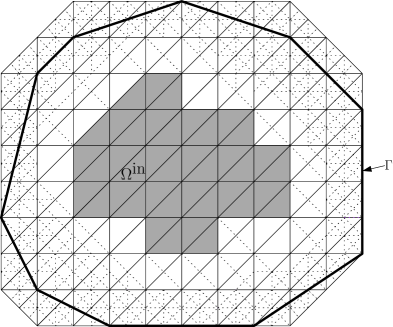
In the CFE method, the domain $\mathrm{\Omega }$ is discretized using coarse-scale and fine-scale grids as shown, see [26].

3.1.1. Refinement of the two-scaled grid:

Let ${𝒯}_H=\{T_1,T_2,\mathrm{\dots },T_n\}$ denote the larger grid consisting of regular triangles of conforming shape, known as coarse-scale grid. The idea for this discretization is given by Ciarlet [8]. For every triangle $T\in {𝒯}_H$, $\text{int}(T)$ indicates the interior of $T$. Since ${𝒯}_H$ is a grid with overlapping elements, we have $\forall T\in {𝒯}_H,\mathrm{\Omega }\subset \bigcup _{T\in {𝒯}_H}T\text{with}\text{int}(T)\cap \mathrm{\Omega }\ne \mathrm{\varnothing }.$

Next, we denote the smaller grid, known as fine-scale grid using the notation ${𝒯}_h$. The boundary $\mathrm{\Gamma }$ of the domain is discretized by the fine-scale grid and it exclusively consists of the slave nodes, which are employed to conform the shape functions to satisfy the Dirichlet boundary conditions. The coarse-scale grid ${𝒯}_H$ contains the degrees of freedom and the fine-scale grid ${𝒯}_h$ contains the slave nodes only.

3.1.2. Boundary adaptation:

The diameter of any given triangle $T$ within ${𝒯}_H$ is represented by the notation $h_T$. The size of the coarse-scale mesh given by $H$ is defined as $H:=\max \{h_T:T\in {𝒯}_H\}$. i.e., it indicates the largest diameter of the triangle. Let ${𝒯}_{H,h}$ be the two-scale triangulation. In the neighborhood of $\mathrm{\Gamma }$, the triangles near the boundary will be refined. The refinement by the finer-scale is carried out for several iterations and the stopping criteria is given as

(3) $\text{dist}(T,\mathrm{\Gamma })\le {\sigma }_{\text{dist}}{h}_T\forall T\in {𝒯}_{H,h}\setminus {𝒯}_H^{\text{in}},$

where the positive parameter ${\sigma }_{\text{dist}}$ governs the width of this particular neighborhood. For any $T\in {𝒯}_H$, $\text{sons}(T)$ which indicates the set of sons, is specified by $\text{sons}(T):=\{\tau \in {𝒯}_{H,h}:\tau \subset T\}.$ To obtain $\tau$ (sons of $T$), we divide each $T$ into four triangles by connecting the mid points of the edges of $T$ and define $n_T:=\mathrm{♯}\text{sons}(T)$. This process yields a new grid that exhibits a higher level of refinement than ${𝒯}_H$, conforming and shape regular. Also, in the interior of $\mathrm{\Omega }$, it does not differ from ${𝒯}_H$. The fine-scale grid size $h$ is defined as $h:=\min \{h_{\tau }:\tau \in {𝒯}_{H,h}\},h\le H$. In the neighborhood of $\mathrm{\Gamma }$, the fine-scale parameter $h$ serves as a defining characteristic of the two-scale mesh ${𝒯}_{H,h}$.

3.1.3. Degrees of freedom

Next, we establish the submesh ${𝒯}_H^{\text{in}}$ within the interior part of the domain, at a certain distance from $\mathrm{\Gamma }$, using the following definition

${𝒯}_H^{\text{in}}:=\{\tau \in \text{sons}(T):T\in {𝒯}_H\setminus {𝒯}_{\mathrm{\Gamma }}\}\subset {𝒯}_{H,h},$

by considering the coarse-scale parameter $H$ and the fine-scale parameter $h$, where ${𝒯}_{\mathrm{\Gamma }}$ is a subset of ${𝒯}_H$ which consists of all the triangles near the boundary. In order to locate the degrees of freedom, we check on the free nodes. It is calculated based on the corresponding vertices in the coarse mesh ${𝒯}_H^{\text{in}}$, which means that it relies on the inner mesh ${𝒯}_H^{\text{in}}$. Suppose ${\vartheta }_H$ be the set of all vertices in ${𝒯}_H$. Then we define the degrees of freedom as follows

${\vartheta }_{\text{d}}:=\{x\in 𝐆(T):T\in {𝒯}_H^{\text{in}}\}.$

The values at the nodes $x\in {\vartheta }_{\text{d}}$ gives the values of the CFE functions. Thus, the minimal number of unknowns in the CFE method remains unaffected by the count of the geometric details or their size. In short, the dimension of the CFE space is not affected by the finer-scale grid.

3.1.4. Indicating slave nodes

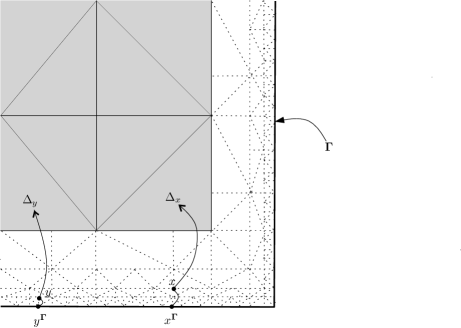
We now know that the function values are constrained at the slave nodes. For the given Dirichlet boundary conditions, we use the grid points and form the triangles for adapting the shape of the CFE functions. All the nodes in ${𝒯}_{H,h}$, apart from the free nodes are termed as slave nodes (Refer to Fig. 2). As mentioned above, let the set of all vertices of the two scale mesh be denoted by the notation ${\vartheta }_{H,h}$. Then we define the slave nodes as follows

${\vartheta }_{\text{s}}:={\vartheta }_{H,h}\setminus {\vartheta }_{\text{d}}.$

Since the degrees of freedom are located at the inner mesh ${𝒯}_H^{\text{in}}$, we use extrapolation method to determine the values at the slave nodes of the two-scale mesh.

Figure 1. Discretization using the CFE method for the two-scale grid ${𝒯}_{H,h}$.The inner triangulation ${𝒯}_H^{\text{in}}$ comprises the degrees of freedom. It is denoted by the dark shaded triangles. The triangles near the boundary are represented with the dotted lines which consists of the slave nodes.

Figure 2. The black line indicate the boundary $\mathrm{\Gamma }$. The selection of the closest inner simplex ${\mathrm{\Delta }}_x$ and ${\mathrm{\Delta }}_y$, and the closest boundary point $x^{\mathrm{\Gamma }}$ and $y^{\mathrm{\Gamma }}$, respectively for the slave nodes $x$ and $y$ is shown.

3.1.5. Extrapolation operator

As mentioned above, in order to calculate slave node values, we define an extrapolation operator. On the boundary, each slave node $x\in {\vartheta }_{\text{s}}$ depends on the closer coarse grid triangle ${\mathrm{\Delta }}_x\in {𝒯}_H^{\text{in}}$ and the closest point $x^{\mathrm{\Gamma }}$ on the boundary $\mathrm{\Gamma }$ (see Fig. 2).

As the inner nodes ${\vartheta }_{\text{d}}$ contain the degrees of freedom, we first assume a grid function $𝚽:{\vartheta }_{\text{d}}\to ℝ$ to define the extrapolation operator. For any triangulation $T\in {𝒯}_H$, there exists a linear function ${\varphi }_T\in {\mathbb{P}}_1({ℝ}^2)$ which is uniquely determined and interpolates $𝚽$ in the vertices of $T$, where ${\mathbb{P}}_1({ℝ}^2)$ denotes the space of bivariate polynomials on ${ℝ}^2$ of maximal degree $1$. The extension value of $𝚽$ at a slave node $x\in {\vartheta }_{\text{s}}$ is defined by ${(ℰ𝚽)}_x:={\varphi }_{{\mathrm{\Delta }}_x}(x)-{\varphi }_{{\mathrm{\Delta }}_x}(x^{\mathrm{\Gamma }}).$ The extrapolation operator $ℰ:{ℝ}^{{\vartheta }_{\text{d}}}\to {ℝ}^{{\vartheta }_{H,h}}$ for the grid functions is defined as

(4)

where ${\sigma }_{\text{ds}}>0$ is some parameter. We now summarize the notations and their precise definitions below:

${𝒯}_{H,h}$	The two-scale grid triangulation, with grid size $H$ and $h$
${\vartheta }_{H,h}$	The set of mesh points corresponding to the two-scale grid
${𝒯}_H$	The coarse grid triangulations that initially overlap
${\vartheta }_H$	The set of vertices corresponding to the coarse grid triangulations
${\sigma }_{\text{dist}}$	Positive width control parameter
$\text{sons}(T)$	Refined triangles of $T$
${𝒯}_H^{\text{in}}$	The inner portion of the grid of the two-scaled triangulation ${𝒯}_{H,h}$
${\vartheta }_{\text{d}}$	The set of vertices which corresponds to ${𝒯}_H^{\text{in}}$ (degrees of freedom)
${𝒯}_{\mathrm{\Gamma }}$	The set of all triangles near to the boundary, ${𝒯}_{\mathrm{\Gamma }}\subset$ ${𝒯}_H$
${\vartheta }_{\text{s}}$	The set of all slave nodes acquired as ${\vartheta }_{\text{d}}$ removed from ${\vartheta }_{H,h}$
$ℰ$	Extrapolation operator
$T$	Triangle (closed)
$\tau$	sons($T$)
${\mathrm{\Delta }}_x$	For $x\in {\vartheta }_{\text{s}}$, ${\mathrm{\Delta }}_x\in {𝒯}_H^{\text{in}}$ has minimum distance to $x$
$x^{\mathrm{\Gamma }}$	For $x\in {\vartheta }_{\text{s}}$, $x^{\mathrm{\Gamma }}\in \mathrm{\Gamma }$ has minimum distance to $x$
$𝐆(T)$	The set of vertices of a triangle $T$
$n_T$	Number of sub-triangles in $T\in {𝒯}_{\mathrm{\Gamma }}$
${\sigma }_{\text{ds}}$	Distance control parameter

Due to the domain discretization, some geometric constants will be involved in our context, such as ${\sigma }_{\text{uni}},{𝒯}_{\text{ol}}(\tau ),{𝒞}_{\text{ol,1}},{𝒞}_{\text{ol,2}}\text{ and }{\sigma }_{\text{ext}}$. For details about these constants, please refer to [23].

Remark 1.

One-scale CFE method: In this method $T$ is not subdivided, i.e., $n_T=1$ and then the two-scale grid ${𝒯}_{H,h}$ corresponds to the coarse mesh ${𝒯}_H$ $(h=𝒪(H))$. In the case where $h\ll H$, this is called two-scale CFE method.

3.2. The domain and the solution space

We define the space $S$ which is continuous. The piecewise linear finite element space $S$ is defined on the mesh ${𝒯}_{H,h}$ as $S:=\{v\in C^0({\mathrm{\Omega }}_{H,h}):{v|}_T\in {\mathbb{P}}_1\forall T\in {𝒯}_{H,h}\},$ where ${\mathrm{\Omega }}_{H,h}:=\text{int}\left({\bigcup }_{T\in {𝒯}_{H,h}}T\right)$. Now, considering the two-scale approximation of the Dirichlet boundary condition on the triangulations ${𝒯}_{H,h}$, the CFE space denoted by $S^{\text{CFE}}$ (which is a subspace of $S$) can be defined as follows

$S^{\text{CFE}}:=\{v\in S:\exists 𝚽\in {ℝ}^{{\vartheta }_{\text{d}}}\text{with}v(x)={(ℰ𝚽)}_x\forall x\in {\vartheta }_{H,h}\}.$

3.3. CFE Basis Function

Considering the solution space $S^{\text{CFE}}$, we need to define the basis function. For that, let $S^{\text{in}}$ be the piecewise linear finite element space which is continuous. Let $S^{\text{in}}$ be defined on the inner grid ${𝒯}_H^{\text{in}}$.

$S^{\text{in}}:=\{u\in C^0({\mathrm{\Omega }}^{\text{in}})\mid {u|}_T\in {\mathbb{P}}_1\forall T\in {𝒯}_H^{\text{in}}\},$

where the interior ${\mathrm{\Omega }}^{\text{in}}:=\text{int}\left({\bigcup }_{T\in {𝒯}_H^{\text{in}}}T\right)$. According to (4), the extrapolation operator is a mapping $ℰ:S^{\text{in}}\to S$. Corresponding to this extrapolation operator, the CFE space can be written as

$S^{\text{CFE}}=ℰ(S^{\text{in}})\subset S.$

For the finite element space $S^{\text{in}}$, we define the standard nodal basis function ${\{{\varrho }_i\}}_{i=1}^{N^{\text{CFE}}}$ along with the property

${\varrho }_i(x_j)={\delta }_{ij}\forall \mathrm{\hspace{0.33em}1}\le i,j\le N^{\text{CFE}},\text{ with }{\delta }_{ij}=\{\begin{array}{cc}1,\text{if}i=j,\hfill & \\ 0,\text{if}i\ne j.\hfill & \end{array}$

where the dimension of solution space $S^{\text{CFE}}$ is given by $N^{\text{CFE}}$ and the degrees of freedom (free nodes in ${𝒯}_H^{\text{in}}$) is given by ${\vartheta }_{\text{d}}=\{x_j:\mathrm{\hspace{0.25em}1}\le j\le N^{\text{CFE}}\}$. Now, we consider the CFE Solution space $S^{\text{CFE}}$.
For this space we define the nodal basis functions as

${\varphi }_i^{\text{CFE}}:=ℰ[{\varrho }_i]\in S^{\text{CFE}}\forall \mathrm{\hspace{0.33em}1}\le i\le N^{\text{CFE}}.$

Here also, we assume CFE basis function ${\varphi }_i^{\text{CFE}}$ corresponding to each free node $x_i\in {\vartheta }_{\text{d}}$ as

${\varphi }_i^{\text{CFE}}(x_j)={\delta }_{ij}\forall \mathrm{\hspace{0.33em}1}\le i,j\le N^{\text{CFE}}.$

Remark 2.

$N^{\text{CFE}}$ is determined by the degrees of freedom, i.e., the number of nodes in ${\vartheta }_{\text{dof}}$. It is independent of the slave nodes ${\vartheta }_{\text{s}}$. Hence, dimension of $S^{\text{CFE}}\ll$ dimension of $S$.

4. Semilinear problem

The weak or variational formulation of the problem described in (1) is written as: For each $t\in I$, find $u(t)\in H_0^1(\mathrm{\Omega })$ such that

(5) $(u_t,\varphi )+(\nabla u,\nabla \varphi )$ $=(f(u),\varphi )\forall \varphi \in H_0^1(\mathrm{\Omega }),t\in I,$

$u(0)$ $=v(x).$

Let $u^{\text{CFE}}:\overline{I}\to S^{\text{CFE}}$ be the solution of the given problem, defined as

(6) $(u_t^{\text{CFE}},\chi )+(\nabla u^{\text{CFE}},\nabla \chi )$ $=(f(u^{\text{CFE}}),\chi )\forall \chi \in S^{\text{CFE}},t\in I,$

$u^{\text{CFE}}(0)$ $=v^{\text{CFE}},$

where $v^{\text{CFE}}$ is a suitable approximation of $v$ in $S^{\text{CFE}}.$

4.1. CFE solution: Existence and uniqueness

We have already introduced the CFE basis functions $\left\{{\varphi }_j^{\text{CFE}};\mathrm{\hspace{0.33em}1}\le j\le N^{\text{CFE}}\right\}$. Since the solution $u^{\text{CFE}}(\cdot ,t)$ belongs to the space $S^{\text{CFE}}$, it can be represented in terms of the basis functions as

$u^{\text{CFE}}(x,t)$ $={\displaystyle \sum _{j=1}^{N^{\text{CFE}}}}{\alpha }_j(t){\varphi }_j^{\text{CFE}}(x).$

The semidiscrete CFE approximation is to find the coefficients ${\alpha }_j$’s such that (6) become

(7)

for $\chi ={\varphi }_k^{\text{CFE}},k=1,2,3,\mathrm{\dots },N^{\text{CFE}}$ and ${\gamma }_j,j=1,2,\mathrm{\dots },N^{\text{CFE}}$ are the components of the given initial approximation $v^{\text{CFE}}.$ Setting $\alpha$ as the vector of unknowns

$${\alpha }_j(t)={[{\alpha }_1(t),{\alpha }_2(t),\mathrm{\dots },{\alpha }_{N^{\text{CFE}}}(t)]}^T$$

and considering the mass matrix $B=(b_{jk})$ and the stiffness matrix $A=(a_{jk})$ with the elements $b_{jk}=({\varphi }_j^{\text{CFE}},{\varphi }_k^{\text{CFE}})$ and $a_{jk}=(\nabla {\varphi }_j^{\text{CFE}},\nabla {\varphi }_k^{\text{CFE}})$. The vector $\tilde{f}(\alpha )=({\tilde{f}}_k(\alpha ))$ with entries ${\tilde{f}}_k(\alpha )=(f({\sum }_{j=1}^{N^{\text{CFE}}}{\alpha }_j(t){\varphi }_j^{\text{CFE}}),{\varphi }_k^{\text{CFE}})$ and let $\gamma =({\gamma }_k).$

Then Equation (7) becomes

$$B{\alpha }^{\prime }(t)+A\alpha (t)=\tilde{f}(\alpha ),\text{ for }t\in I,\text{ with }\alpha (0)=\gamma .$$

$A$ and $B$ are positive definite matrices and $\tilde{f}(\alpha )$ is Lipschitz continuous on ${ℝ}^{N^{\text{CFE}}}$. We determine ${\alpha }_n={\alpha }_n(t),n=1,2,\mathrm{\dots }$ from the given iterative scheme as

$B{\alpha }_{n+1}^{\prime }(t)+A{\alpha }_{n+1}(t)$ $=\tilde{f}({\alpha }_n)\text{ for }t\in I,\text{ with }{\alpha }_{n+1}(0)=\gamma ,\text{ for }n\ge 0,$

${\alpha }_0(t)$ $\equiv \gamma \text{ on }\overline{I}.$

This follows that for any $t\in I$, the system posseses a unique and bounded solution ${\alpha }_n$.

4.2. Error Estimation

In this section, we examine the semidiscrete error analysis in CFE framework for smooth initial data. The discretization is carried out only for the space coordinates. For the analysis of the error, we define the Elliptic projection also known as Ritz projection $R^{\text{CFE}}$ onto the solution space $S^{\text{CFE}}$. The orthogonal projection $R^{\text{CFE}}$ with respect to the inner product $(\nabla v,\nabla w)$ defined as

(8) $(\nabla R^{\text{CFE}}v,\nabla \chi )=(\nabla v,\nabla \chi )\forall \chi \in S^{\text{CFE}},\text{ for}v\in H_0^1.$

For $\chi =R^{\text{CFE}}v$ in (8), we obtain $\Vert \nabla R^{\text{CFE}}v\Vert \le \Vert \nabla v\Vert \forall v\in H_0^1.$ Therefore, the elliptic projection is stable in $H^1$ norm.

Before starting the error analysis, we need the estimation of the elliptic projection (see Lemma 4). For the detailed proof which has been estimated in the CFE framework, please refer to [23]. The estimation of the elliptic projection involves the term $\tilde{\log }(H/h)$, which is defined in the following remark.

Remark 3.

We define

$$\tilde{\log }(H/h):=\max \{\widehat{\log }(h_T/h_T^{\min }):T\in {𝒯}_{\mathrm{\Gamma }}\},$$

where

$$\widehat{\log }(h_T/h_T^{\min }):={𝒞}_{\text{ol},1}\underset{\tau \in \text{sons}(T)}{\max }(1+\log (h_T/h_{\tau }))\ge {𝒯}_{\text{ol}}(\tau ),\forall T\in {𝒯}_{\mathrm{\Gamma }}.$$

For the proof of the above inequality and the details about $\widehat{\log }(h_T/h_T^{\min })$, see [26]. The above inequality will be used in the proof of Lemma 4.

We are now prepared to state Lemma 4, which is given as follows.

Lemma 4.

Let $v\in H_0^1(\mathrm{\Omega })\cap H^2(\mathrm{\Omega })$ and $R^{\text{CFE}}$ be defined by (8). Suppose that the condition (3) holds true. Then there exists a positive constant C depending on the ${\sigma }_{\text{dslave}},{\sigma }_{\text{dist}},{\sigma }_{\text{uni}},{𝒯}_{\text{ol}}(\tau ),{𝒞}_{\text{ol,1}},{𝒞}_{\text{ol,2}}\text{ and }{\sigma }_{\text{ext}}$ and the minimal angle in the triangulation ${𝒯}_{H,h}$, such that

$$\Vert \nabla (R^{\text{CFE}}v-v)\Vert \le CH{\tilde{\log }}^{1/2}(H/h){\Vert v\Vert }_{2,\mathrm{\Omega }}$$

and

$$\Vert (R^{\text{CFE}}v-v)\Vert \le C{H}^2\tilde{\log }(H/h){\Vert v\Vert }_{2,\mathrm{\Omega }}.$$

4.3. Semidiscrete error estimates

In the present section, we focus on the semidiscrete error estimates and hence we concentrate on bounding the error term ($u^{\text{CFE}}(t)-u(t)$) for each $t\in \overline{I}$ in both the $L^2$ and $H^1$ norm. The CFE error estimate for spatially discrete case in the $L^2$ norm (for each time level) is given as follows.

Theorem 5.

Let $u(t)$ and $u^{\text{CFE}}(t)$ be the solutions of Equations (1) and (6), respectively and $u(t),u_t(t)\in H_0^1(\mathrm{\Omega })\cap H^2(\mathrm{\Omega })$ for each $t$. Assume that the condition (2) holds true. Then there exists a positive constant $C=C(u,\overline{t})$ independent of $h$ and $H$ such that for appropriately chosen $v^{\text{CFE}}$, we have

$$\Vert u^{\text{CFE}}(t)-u(t)\Vert \le C{H}^2\tilde{\log }(H/h),\text{for}t\in \overline{I}.$$

Proof.

For estimating the error, we use the Energy Argument. We split the error term $\left(u^{\text{CFE}}(t)-u(t)\right)$ as follows

(9) $$u^{\text{CFE}}(t)-u(t)=\left(u^{\text{CFE}}(t)-R^{\text{CFE}}u(t)\right)+\left(R^{\text{CFE}}u(t)-u(t)\right).$$

We put the first part as $\theta$ and the second part as $\rho$, i.e., $\theta =u^{\text{CFE}}(t)-R^{\text{CFE}}u(t)$ and $\rho =R^{\text{CFE}}u(t)-u(t)$. Then Equation (9) becomes

$$u^{\text{CFE}}(t)-u(t)=\theta (t)+\rho (t).$$

From Lemma 4, we get $\rho (t)$ and ${\rho }_t(t)$ bounded as follows:

$$\Vert \rho (t)\Vert \le \overline{C}{H}^2\tilde{\log }(H/h){\Vert u\Vert }_{2,\mathrm{\Omega }}=C{H}^2\tilde{\log }(H/h),$$

and

$$\Vert {\rho }_t(t)\Vert \le \overline{C}{H}^2\tilde{\log }(H/h){\Vert u_t\Vert }_{2,\mathrm{\Omega }}=C{H}^2\tilde{\log }(H/h),$$

where $C$ is depending on $u$.

Next we need to bound $\theta (t)$. Using Equation (6), we obtain

$({\theta }_t,\chi )+(\nabla \theta ,\nabla \chi )$ $=(u_t^{\text{CFE}}-R^{\text{CFE}}{u}_t,\chi )+(\nabla (u^{\text{CFE}}-R^{\text{CFE}}u),\nabla \chi )$

$=(u_t^{\text{CFE}},\chi )+(\nabla u^{\text{CFE}},\nabla \chi )-(R^{\text{CFE}}{u}_t,\chi )-(\nabla R^{\text{CFE}}u,\nabla \chi )$

$=(f(u^{\text{CFE}}),\chi )-(R^{\text{CFE}}{u}_t,\chi )-(\nabla R^{\text{CFE}}u,\nabla \chi ),$

adding and subtracting the term $(u_t,\chi )$ together with (5) and the definition of Ritz projection (8), we have

(10) $({\theta }_t,\chi )+(\nabla \theta ,\nabla \chi )=(f(u^{\text{CFE}})-f(u),\chi )-({\rho }_t,\chi ).$

Substituting $\chi =\theta$ and using (2), together with the usage of Friedrichs’ inequality $\Vert \theta \Vert \le \Vert \nabla \theta \Vert$ (cf. [29]), we obtain

$\frac{1}{2}\frac{d}{dt}{\Vert \theta \Vert }^2+{\Vert \nabla \theta \Vert }^2$ $=(f(u^{\text{CFE}})-f(u),\theta )-({\rho }_t,\theta )$

$\le |f(u^{\text{CFE}})-f(u),\theta |+|{\rho }_t,\theta |$

$\le C\Vert u^{\text{CFE}}(t)-u(t)\Vert \Vert \nabla \theta \Vert +\Vert {\rho }_t\Vert \Vert \theta \Vert$

$\le C({\Vert \theta \Vert }^2+{\Vert \rho \Vert }^2+{\Vert {\rho }_t\Vert }^2)+{\Vert \nabla \theta \Vert }^2,$

where in the last step we have used the Hölder’s inequality. This gives

$\frac{1}{2}\frac{d}{dt}{\Vert \theta \Vert }^2$ $\le C({\Vert \theta \Vert }^2+{\Vert \rho \Vert }^2+{\Vert {\rho }_t\Vert }^2),$

integrating we have

${\Vert \theta (t)\Vert }^2\le {\Vert \theta (0)\Vert }^2+C{\displaystyle {\int }_0^t}({\Vert \theta \Vert }^2+{\Vert \rho \Vert }^2+{\Vert {\rho }_t\Vert }^2)𝑑s,$

using Gronwall’s lemma, the above equation shows

(11) ${\Vert \theta (t)\Vert }^2\le {\Vert \theta (0)\Vert }^2+C{\displaystyle {\int }_0^t}({\Vert \rho \Vert }^2+{\Vert {\rho }_t\Vert }^2)𝑑s,$

where $C$ now depends on $\overline{t}$ [29]. It is easy to observe that

$$\Vert \theta (0)\Vert \le \Vert v^{\text{CFE}}-v\Vert +\Vert R^{\text{CFE}}v-v\Vert \le \Vert v^{\text{CFE}}-v\Vert +C{H}^2\tilde{\log }(H/h){\Vert v\Vert }_{2,\mathrm{\Omega }}.$$

Substituting the values of $\Vert \theta (0)\Vert$, (11) gives

${\Vert \theta (t)\Vert }^2\le C{\Vert v^{\text{CFE}}-v\Vert }^2+C{H}^4{\tilde{\log }}^2(H/h),$

which shows

$\Vert \theta (t)\Vert \le C\Vert v^{\text{CFE}}-v\Vert +C{H}^2\tilde{\log }(H/h).$

Therefore, using the bound of $\theta (t)$ together with the bound of $\rho (t)$ one can obtain the required estimate, which completes the proof. ∎

Next, our aim is to find the error estimate in the gradient norm. For finding the estimate in gradient norm, we will use some inequality for the estimation of $(f(u^{\text{CFE}})-f(u))$, given as the following remark.

Remark 6.

Following the argument of [29], choose $q$ with 2. We have ${\Vert \theta \Vert }_{L^q}\le C\Vert \nabla \theta \Vert$ and the Hölder’s inequality $q^{-1}+{(q^{\prime })}^{-1}=$1,

$$|f(u^{\text{CFE}})-f(u),\theta |\le C\parallel f(u^{\text{CFE}})-f(u){\parallel }_{L^{q^{\prime }}}\parallel \nabla \theta \parallel .$$

With using the assumption $|f^{\prime }(u)|\le C\left(1+{|u|}^p\right)$, for $u\in ℝ$ (as done in Thomée [29, Ch. 14, eq. (14.5)] and applying the Hölder’s inequality once again with exponents $2/q^{\prime }$ and $2/(2-q^{\prime })$, we obtain

${\Vert f(u^{\text{CFE}})-f(u)\Vert }_{L^{q^{\prime }}}^{q^{\prime }}$ $\le C{\displaystyle {\int }_{\mathrm{\Omega }}}{|u^{\text{CFE}}-u|}^{q^{\prime }}{\left(1+|u^{\text{CFE}}|+|u|\right)}^{p{q}^{\prime }}𝑑x$

$\le C{\Vert u^{\text{CFE}}-u\Vert }^{q^{\prime }}{\left(1+{\Vert u^{\text{CFE}}\Vert }_{L^s}+{\Vert u\Vert }_{L^s}\right)}^{p{q}^{\prime }}$

with $s=2pq/(q-2)$. Since $u$ is smooth and , we have ${\Vert u^{\text{CFE}}\Vert }_{L^s}\le C\Vert \nabla u^{\text{CFE}}\Vert$, we can conclude that

$${\Vert f(u^{\text{CFE}})-f(u)\Vert }_{L^{q^{\prime }}}\le C\Vert u^{\text{CFE}}-u\Vert {\left(1+\Vert \nabla u^{\text{CFE}}\Vert \right)}^p.$$

Note that, the inequality $|f^{\prime }(u)|\le C(1+{|u|}^p)$ is more restrictive than the first inequality (1.2), as it implies an upper bound on $|f^{\prime }(u)|$ that depends on $u$. Therefore, the value of $B$ should be chosen to accommodate the maximum possible value of $|f^{\prime }(u)|$ for all values of $u$, considering the more restrictive inequality. Henceforth, it is enough to choose $(1+{|u|}^p)\le B/C$, which easily follows the inequality (1.2)???.

Theorem 7.

Let $u(t)$ be the solution of (1) and $u^{\text{CFE}}(t)$ be the solution of Equation (6). Assume $u(t)\text{ and }{u}_t(t)\text{ belongs to }{H}_0^1(\mathrm{\Omega })\cap H^2(\mathrm{\Omega })$ for each $t$. Let the boundedness condition (2) holds. If $v^{\text{CFE}}=R^{\text{CFE}}v$, there exists a positive constant $C=C(u,\overline{t})$ independent of the mesh parameters $(h,H)$, such that the inequality holds

$$\Vert \nabla (u^{\text{CFE}}(t)-u(t))\Vert \le CH{\tilde{\log }}^{1/2}(H/h),\text{for}t\in \overline{I}.$$

Proof.

Computing in the similar manner as in the proof of Theorem 5 and substituting $\chi =2{\theta }_t$ in Equation (10), we get

$2{\Vert {\theta }_t\Vert }^2+\frac{d}{dt}{\Vert \nabla {\theta }_t\Vert }^2=2(f(u^{\text{CFE}})-f(u),{\theta }_t)-2({\rho }_t,{\theta }_t),$

apply kickback on the term of $2{\Vert {\theta }_t\Vert }^2$,

$\frac{d}{dt}{\Vert \nabla \theta \Vert }^2$ $\le {\Vert f(u^{\text{CFE}})-f(u)\Vert }^2+{\Vert {\rho }_t\Vert }^2$

(12) $\le 2{\Vert f(u^{\text{CFE}})-f(R^{\text{CFE}}u)\Vert }^2+2{\Vert f(R^{\text{CFE}}u)-f(u)\Vert }^2+C{H}^2\tilde{\log }(\frac{H}{h}).$

Now following the similar estimates of $(f(u^{\text{CFE}})-f(u))$ as in Remark 6,

${\Vert f(R^{\text{CFE}}u)-f(u)\Vert }^2$ $\le C{\displaystyle {\int }_{\mathrm{\Omega }}}{\left(R^{\text{CFE}}u-u\right)}^2{\left(1+|R^{\text{CFE}}u|\right)}^{2p}𝑑x$

$=C{\displaystyle {\int }_{\mathrm{\Omega }}}{\rho }^2{\left(1+|R^{\text{CFE}}u|\right)}^{2p}𝑑x$

$\le C{\left({\displaystyle {\int }_{\mathrm{\Omega }}}{\rho }^q𝑑x\right)}^{2/q}{\left({\displaystyle {\int }_{\mathrm{\Omega }}}{\left(1+|R^{\text{CFE}}u|\right)}^s𝑑x\right)}^{(q-2)/q}$

$\le C{\Vert \rho \Vert }_{L^q}^2{\left(1+{\Vert R^{\text{CFE}}u\Vert }_{L^s}\right)}^{2p}$

(13) $\le C{\Vert \nabla \rho \Vert }^2\le C{H}^2\tilde{\log }(H/h),$

here we have used ${\Vert R^{\text{CFE}}u\Vert }_{L^s}\le C\Vert \nabla R^{\text{CFE}}u\Vert \le C\Vert \nabla u\Vert \le C$. In the similar way, we have

${\Vert f(u^{\text{CFE}})-f(R^{\text{CFE}}u)\Vert }^2$ $\le C{\Vert \nabla \theta \Vert }^2{\left(1+\Vert \nabla u^{\text{CFE}}\Vert \right)}^{2p}$

(14) $\le C{\Vert \nabla \theta \Vert }^2{\left(1+\Vert \nabla \theta \Vert \right)}^{2p}.$

Using Equations (13) and (14), we obtain from (12)

(15) $\frac{d}{dt}{\Vert \nabla \theta \Vert }^2\le C{\Vert \nabla \theta \Vert }^2{\left(1+\Vert \nabla \theta \Vert \right)}^{2p}+C{H}^2\tilde{\log }(H/h).$

Assume $t_H\in \overline{I}$ is as large as possible with $\Vert \nabla \theta \Vert \le 1$ on $[0,{\overline{t}}_H]$. Then for $t\le {\overline{t}}_H,$ from Equation (15) we have,

(16) $\frac{d}{dt}{\Vert \nabla \theta \Vert }^2$ $\le C{\Vert \nabla \theta \Vert }^2+C{H}^2\tilde{\log }(H/h),$

with $C$ independent of ${\overline{t}}_H$, this gives

$$\Vert \nabla \theta \Vert \le CH{\tilde{\log }}^{1/2}(H/h)e^{C\overline{t}}\le \frac{1}{2},\text{ for }H\le H_0.$$

It follows that ${\overline{t}}_H=\overline{t}$ for $H\le H_0$ (since $h\ll H$ and using Remark 3), so that $\Vert \nabla \theta \Vert \le 1$ on $\overline{I}$ for these $H$ and therefore,

$$\Vert \nabla u^{\text{CFE}}\Vert \le \Vert \nabla u\Vert +1\text{ on }\overline{I}.$$

Therefore, our claim $\Vert \nabla \theta \Vert \le 1$ is fulfilled in order to obtain Equation (16). Now, (16) gives after integration

${\Vert \nabla \theta (t)\Vert }^2\le {\Vert \nabla \theta (0)\Vert }^2+C{\displaystyle {\int }_0^t}\left({\Vert \nabla \theta \Vert }^2+H^2\tilde{\log }(H/h)\right)𝑑s,$

using Gronwall’s lemma, the above equation gives

${\Vert \nabla \theta (t)\Vert }^2\le {\Vert \nabla \theta (0)\Vert }^2+C{\displaystyle {\int }_0^t}\left(H^2\tilde{\log }(H/h)\right)𝑑s,$

where $C$ now depends on $\overline{t}$. Then for $v^{\text{CFE}}=R^{\text{CFE}}v$, we obtain $\Vert \nabla \theta (t)\Vert \le CH{\tilde{\log }}^{1/2}(H/h)$. Altogether the bound of $\nabla \rho (t)$ concludes the proof of the theorem. ∎

Remark 8.

Note that when $h=𝒪(H)$, the two-scale grid ${𝒯}_{H,h}$ coincides with the coarse grid ${𝒯}_H$, and the results of Theorems 5 and 7 coincides with the standard FEM [29].

5. Fully discrete error estimates

Next, we examine the variation/discretization in both the space and time constraints. Let $U^{\text{CFE, }n}=U^n$ be an approximation of $u(t_n)=u^n$. Here also, we bound the error term $U^n-u^n$ in the $L^{\mathrm{\infty }}(L^2)$-norm. We use two approaches for finding the error estimates- The backward Euler and the Crank-Nicolson method.

5.1. Backward Euler method

The variational form is similar to Equation (6), but in both time-space discretization, it is given by

(17) $(\overline{\partial }{U}^n,\chi )+(\nabla U^n,\nabla \chi )=(f(U^n),\chi ),\forall \chi \in S^{\text{CFE}},n\ge 1,U^0=v^{\text{CFE}}.$

Using the backward difference quotient for the term $\overline{\partial }{U}^n$ as $(U^n-U^{n-1})/k$, Equation (17) gives

$$(\frac{U^n-U^{n-1}}{k},\chi )+(\nabla U^n,\nabla \chi )=(f(U^n),\chi ),$$

after simplifying,

(18) $(U^n,\chi )+k(\nabla U^n,\nabla \chi )=(U^{n-1},\chi )+k(f(U^n),\chi ).$

Representing $U^n={\sum }_{j=1}^{N^{\text{CFE}}}{\alpha }^n{\varphi }_j^{\text{CFE}}$ and choosing $\chi ={\varphi }_k^{\text{CFE}}\text{for}k=1,2,3,$
$\mathrm{\dots },N^{\text{CFE}}$, the Equation (18) becomes

${\displaystyle \sum _{j=1}^{N^{\text{CFE}}}}{\alpha }^n({\varphi }_j^{\text{CFE}},{\varphi }_k^{\text{CFE}})+k{\displaystyle \sum _{j=1}^{N^{\text{CFE}}}}{\alpha }^n(\nabla {\varphi }_j^{\text{CFE}},\nabla {\varphi }_k^{\text{CFE}})=$

(19) $={\displaystyle \sum _{j=1}^{N^{\text{CFE}}}}{\alpha }^{n-1}({\varphi }_j^{\text{CFE}},{\varphi }_k^{\text{CFE}})+k(f\left({\displaystyle \sum _{j=1}^{N^{\text{CFE}}}}{\alpha }^n{\varphi }_j^{\text{CFE}}\right),{\varphi }_k^{\text{CFE}}),$

with ${\alpha }^0=\gamma$ given by $v^{\text{CFE}}$. With matrix notation similar to the usage in the semidiscrete situation, Equation (19) can be written as

(20) $(B+kA){\alpha }^n=B{\alpha }^{n-1}+k\tilde{f}({\alpha }^n),\text{with}{\alpha }^0=\gamma ,$

where $A,B$ and $\tilde{f}(\alpha )$ as given before. The argument which explains the existence and uniqueness of the solution for (20) is detailed in [25, ch. 13]. Now we move on to finding the error estimates in the $L^{\mathrm{\infty }}(L^2)$-norm.

Theorem 9.

Let $U^n$ and $u$ be the solutions of Equations (17) and (1), respectively and the condition (2) holds true. Assume $u$ being sufficiently smooth. Then there exists a positive constant $C=C(u,\overline{t})$ independent of the grid parameters $h,H$ such that for appropriately chosen $v^{\text{CFE}}$, we have

$$\Vert U^n-u^n\Vert \le C\Vert v^{\text{CFE}}-v\Vert +C(u)\left(H^2\tilde{\log }(H/h)+k\right)$$

for $k\le H$ and $t_n\in I.$

Proof.

Proceeding in a similar manner as given in the proof of Theorem 5, we use Energy Argument and split the error in two terms ${\theta }^n=(U^n-R^{\text{CFE}}{u}^n)$ and ${\rho }^n=(R^{\text{CFE}}{u}^n-u^n)$. Since ${\rho }^n$ is bounded by Lemma 4, we proceed with checking the boundedness of ${\theta }^n$.

Using Equation (17) and Ritz projection (8), we write as follows

$(\overline{\partial }{\theta }^n,\chi )+(\nabla {\theta }^n,\nabla \chi )$ $=(f(U^n),\chi )-(\overline{\partial }{R}^{\text{CFE}}{u}^n,\chi )-(\nabla R^{\text{CFE}}{u}^n,\nabla \chi )$

$=(f(U^n),\chi )-(\overline{\partial }{R}^{\text{CFE}}{u}^n,\chi )-(\nabla u^n,\nabla \chi ),$

adding and subtracting the terms $(u_t^n,\chi )$ and $(\overline{\partial }{u}^n,\chi ),$ and calculating we get

$(\overline{\partial }{\theta }^n,\chi )+(\nabla {\theta }^n,\nabla \chi )$ $=(f(U^n)-f(u^n),\chi )-(\overline{\partial }{\rho }^n,\chi )-(\partial u^n-u_t^n,\chi ).$

Put $\chi ={\theta }^n$ and using (2),

$\frac{1}{2}\overline{\partial }{\Vert {\theta }^n\Vert }^2+{\Vert \nabla {\theta }^n\Vert }^2$ $=(f(U^n)-f(u^n),{\theta }^n)-(\overline{\partial }{\rho }^n,{\theta }^n)-(\overline{\partial }{u}^n-u_t^n,{\theta }^n)$

$\le C\left(\Vert U^n-u^n\Vert +\Vert \overline{\partial }{\rho }^n\Vert +\Vert \overline{\partial }{u}^n-u_t^n\Vert \right)\Vert {\theta }^n\Vert$

$\le C\left({\Vert {\rho }^n\Vert }^2+{\Vert \overline{\partial }{\rho }^n\Vert }^2+{\Vert \overline{\partial }{u}^n-u_t^n\Vert }^2\right)+C{\Vert {\theta }^n\Vert }^2$

$=C{\Vert {\theta }^n\Vert }^2+C{M}_n,$

where $M_n={\Vert {\rho }^n\Vert }^2+{\Vert \overline{\partial }{\rho }^n\Vert }^2+{\Vert \overline{\partial }{u}^n-u_t^n\Vert }^2$. Since $\frac{1}{2}\overline{\partial }{\Vert {\theta }^n\Vert }^2\le \frac{1}{2}\overline{\partial }{\Vert {\theta }^n\Vert }^2+{\Vert \nabla {\theta }^n\Vert }^2$, therefore we have

$\overline{\partial }{\Vert {\theta }^n\Vert }^2$ $\le C({\Vert {\theta }^n\Vert }^2+M_n),$

using $\overline{\partial }{\Vert {\theta }^n\Vert }^2=({\Vert {\theta }^n\Vert }^2-{\Vert {\theta }^{n-1}\Vert }^2)/k$,

$(1-Ck){\Vert {\theta }^n\Vert }^2\le {\Vert {\theta }^{n-1}\Vert }^2+Ck{M}_n,$

and for small $k$,

${\Vert {\theta }^n\Vert }^2$ $\le (1+Ck){\Vert {\theta }^{n-1}\Vert }^2+Ck{M}_n,$

$\mathrm{⋮}\mathrm{⋮}$

$\le {(1+Ck)}^n{\Vert {\theta }^0\Vert }^2+Ck{\displaystyle \sum _{j=1}^N}{(1+Ck)}^{n-j}{M}_j,$

(21) $\le C{\Vert {\theta }^0\Vert }^2+Ck{\displaystyle \sum _{j=1}^N}{M}_j.$

For ${\theta }^n$ to be bounded, we have to show $M_j$ is bounded. By Lemma 4, ${\rho }^j$ is bounded. Now,

$$\Vert \overline{\partial }{\rho }^j\Vert =\Vert k^{-1}{\int }_{t_{j-1}}^{t_j}{\rho }_t𝑑s\Vert \le C(u)H^2\tilde{\log }(H/h),$$

and

$\Vert \overline{\partial }{u}^n-u_t^n\Vert =\Vert k^{-1}{\displaystyle {\int }_{t_{j-1}}^{t_j}}(s-t_{j-1})u_{tt}(s)𝑑s\Vert \le C(u)k.$

Altogether we have $M_j\le C(u){(H^2\tilde{\log }(H/h)+k)}^2$. Using the estimation of ${\theta }^0$, we have from (21),

$\Vert {\theta }^n\Vert$ $\le C\Vert v^{\text{CFE}}-v\Vert +C(u)(H^2\tilde{\log }(H/h)+k),$

together with the estimation of ${\rho }^n$ completes the proof. ∎

Remark 10.

It can be noted that the estimate in the $L^{\mathrm{\infty }}(L^2)$-norm is second order convergence in space and first order convergence in time.

In order to avoid the disadvantage of producing system of equations of nonlinear behaviour at each time step, we consider the linearized form of (17)

(22) $(\overline{\partial }{U}^n,\chi )+(\nabla U^n,\nabla \chi )=(f(U^{n-1}),\chi ).\forall \chi \in S^{\text{CFE}},n\ge 1,U^0=v^{\text{CFE}}.$

Applying the backward difference method to the term $\overline{\partial }{U}^n$, we get

$(\frac{U^n-U^{n-1}}{k},\chi )+(\nabla U^n,\nabla \chi )$ $=(f(U^{n-1}),\chi )$

$(U^n,\chi )+k(\nabla U^n,\nabla \chi )$ $=(U^{n-1},\chi )+k(f(U^{n-1}),\chi ).$

Taking $U^n={\sum }_{j=1}^{N^{\text{CFE}}}{\alpha }^n{\varphi }_j^{\text{CFE}}$ and using the positive definiteness property of the matrices $A,B$ we get the unique solution

$${\alpha }^n={(B+kA)}^{-1}\left({\alpha }^{n-1}B+k\tilde{f}({\alpha }^{n-1})\right).$$

Theorem 11.

Let $U^n$ be the solution of Equation (22) and $u$ be the solution of Equation (1). Let the condition (2) holds true. Assume $u$ being sufficiently smooth. Then there exists a positive constant $C=C(u,\overline{t})$ independent of the grid parameters $h,H$ such that for appropriately chosen $v^{\text{CFE}}$, we have

$$\Vert U^n-u^n\Vert \le C\Vert v^{\text{CFE}}-v\Vert +C(u)(H^2\tilde{\log }(H/h)+k)$$

for small $k$, where $k\le H$ and $t_n\in I$.

Proof.

We first concentrate on the boundedness of ${\theta }^n$. This time we obtain the following equation

$(\overline{\partial }{\theta }^n,\chi )+(\nabla {\theta }^n,\nabla \chi )$ $=(f(U^{n-1})-f(u^n),\chi )-(\overline{\partial }{\rho }^n,\chi )-(\overline{\partial }{u}^n-u_t^n,\chi ),$

and substituting $\chi ={\theta }^n$ we obtain

(23) $\frac{1}{2}\overline{\partial }{\Vert {\theta }^n\Vert }^2+{\Vert \nabla {\theta }^n\Vert }^2$ $\le C\left(\Vert U^{n-1}-u^n\Vert +\Vert \overline{\partial }{\rho }^n\Vert +\Vert \overline{\partial }{u}^n-u_t^n\Vert \right)\Vert {\theta }^n\Vert .$

Now we focus on estimating the term $\Vert U^{n-1}-u^n\Vert$. In order to estimate, we add and subtract $R^{\text{CFE}}{u}^{n-1}$ and $u^{n-1}$ to get   $\Vert U^{n-1}-u^n\Vert \le \Vert {\theta }^{n-1}\Vert +\Vert {\rho }^{n-1}\Vert +k\Vert \overline{\partial }{u}^n\Vert$. Using the Friedrich’s inequality, Equation (23) becomes

$\frac{1}{2}\overline{\partial }{\Vert {\theta }^n\Vert }^2+{\Vert \nabla {\theta }^n\Vert }^2\le$

$\le C\left(\Vert {\theta }^{n-1}\Vert +\Vert {\rho }^{n-1}\Vert +k\Vert \overline{\partial }{u}^n\Vert +\Vert \overline{\partial }{\rho }^n\Vert +\Vert \overline{\partial }{u}^n-u_t^n\Vert \right)\Vert \nabla {\theta }^n\Vert ,$

this gives

$\overline{\partial }{\Vert {\theta }^n\Vert }^2$ $\le C{\Vert {\theta }^{n-1}\Vert }^2+C\left({\Vert {\rho }^{n-1}\Vert }^2+k^2{\Vert \overline{\partial }{u}^n\Vert }^2+{\Vert \overline{\partial }{\rho }^n\Vert }^2+{\Vert \overline{\partial }{u}^n-u_t^n\Vert }^2\right)$

$\le C{\Vert {\theta }^{n-1}\Vert }^2+C(u){\left(H^2\tilde{\log }(H/h)+k\right)}^2,$

using $\overline{\partial }{\Vert {\theta }^n\Vert }^2=({\Vert {\theta }^n\Vert }^2-{\Vert {\theta }^{n-1}\Vert }^2)/k$,

${\Vert {\theta }^n\Vert }^2\le (1+Ck){\Vert {\theta }^{n-1}\Vert }^2+C(u)k{\left(H^2\tilde{\log }(H/h)+k\right)}^2,$

after repeated applications and for small $k$,

${\Vert {\theta }^n\Vert }^2$ $\le {(1+Ck)}^n{\Vert {\theta }^0\Vert }^2+C(u)k{\displaystyle \sum _{j=1}^N}{(1+Ck)}^{n-j}{(H^2\tilde{\log }(H/h)+k)}^2,$

$\le C{\Vert {\theta }^0\Vert }^2+C(u){(H^2\tilde{\log }(H/h)+k)}^2.$

Using the estimation of $\Vert {\theta }^0\Vert$ together with the estimation of ${\rho }^n$, the proof is completed. ∎

Now, we move on to Crank-Nicolson method to check for obtaining higher accuracy in time.

5.2. Crank-Nicolson method

Here we take ${\tilde{U}}^n=(U^n+U^{n-1})/2.$ The variational form is similar to Equation (6), but in both time-space discretization, it is given by

(24) $(\overline{\partial }{U}^n,\chi )+(\nabla {\tilde{U}}^n,\nabla \chi )=(f({\tilde{U}}^n),\chi ),\forall \chi \in S^{\text{CFE}},n\ge 1,t_n\in I,U^0=v^{\text{CFE}}.$

Using the definition of both the terms $\overline{\partial }{U}^n$ and ${\tilde{U}}^n$, Equation (24) gives

$$(\frac{U^n-U^{n-1}}{k},\chi )+(\nabla \left(\frac{U^n+U^{n-1}}{2}\right),\nabla \chi )=(f({\tilde{U}}^n),\chi ).$$

It is to be noted that the equation is symmetric around the point $t=t_{n-1/2},$ which indicates the accuracy of second order in time. Multiplying by $2k$ and re-arranging,

$2(U^n,\chi )+k(\nabla U^n,\nabla \chi )=2(U^{n-1},\chi )-k(\nabla U^{n-1},\nabla \chi )+2k(f({\tilde{U}}^n),\chi ),$

therefore similar to the backward Euler method, the nonlinear equation (24) is solvable for $U^n$ in terms of $U^{n-1}$ for small $k$. To avoid the disadvantage of producing nonlinear system of equations at each time step, we consider the linearized modification on the term ${\tilde{U}}^n$ as ${\overline{U}}^n=\frac{3}{2}{U}^{n-1}-\frac{1}{2}{U}^{n-2},$ for $n\ge 2$. Then Equation (24) becomes

(25) $(\overline{\partial }{U}^n,\chi )+(\nabla {\overline{U}}^n,\nabla \chi )=(f({\overline{U}}^n),\chi ),\forall \chi \in S^{\text{CFE}},t_n\in I,$

with $U^0=v^{\text{CFE}}$. The linearized form (25) is always solvable for $U^n$ for the given values of $U^{n-1}$ and $U^{n-2}$.

Now before moving on to the error estimate we define the lemma below. The proof easily follows from [25, ch. 13].

Lemma 12.

Let $R^{\text{CFE}}$ be defined in (8). Assuming the regularity for $u$, we have

$\Vert \nabla R^{\text{CFE}}{u}_{tt}\Vert$ $\le C(u),\text{for }t\in \overline{I}.$

Using this, we find the error estimate.

Theorem 13.

Let $U^n$ be the solution of Equation (24) and $u$ be the solution of Equation (1). Assume that the condition (2) holds true. Then under the regularity assumptions of $u$, there exists a positive constant $C=C(u,\overline{t})$ independent of the grid parameters $h,H$ such that for appropriately chosen $v^{\text{CFE}}$, we have

$$\Vert U^n-u^n\Vert \le C\Vert v^{\text{CFE}}-v\Vert +C(u)(H^2\tilde{\log }(H/h)+k^2)$$

for small $k$, where $k\le H$ and $t_n\in \overline{I}$.

Proof.

The error term is partitioned into two as in the previous cases and ${\rho }^n$ is bounded. It remains to check for ${\theta }^n$. While checking the boundedness, this time we use $(\nabla {\tilde{\theta }}^n,\nabla \chi )$ instead of $(\nabla {\theta }^n,\nabla \chi )$. Using the Ritz projection, we write

$(\overline{\partial }{\theta }^n,\chi )+(\nabla {\tilde{\theta }}^n,\nabla \chi )$ $=(f({\tilde{U}}^n),\chi )-(\overline{\partial }{R}^{\text{CFE}}{u}^n,\chi )-(\nabla R^{\text{CFE}}{\tilde{u}}^n,\nabla \chi ),$

by adding and subtracting the term $(u_t^{n-\frac{1}{2}},\chi )$ to the RHS and rearranging by taking the common terms together, we get as follows.

$(\overline{\partial }{\theta }^n,\chi )+(\nabla {\tilde{\theta }}^n,\nabla \chi )=$

$=(f({\tilde{U}}^n),\chi )-(u_t^{n-\frac{1}{2}},\chi )-(\overline{\partial }{R}^{\text{CFE}}{u}^n-u_t^{n-\frac{1}{2}},\chi )-(\nabla R^{\text{CFE}}{\tilde{u}}^n,\nabla \chi ),$

adding and subtracting $(\nabla R^{\text{CFE}}{u}^{n-\frac{1}{2}},\nabla \chi )$,

$(\overline{\partial }{\theta }^n,\chi )+(\nabla {\tilde{\theta }}^n,\nabla \chi )=$

$=(f({\tilde{U}}^n),\chi )-(\overline{\partial }{R}^{\text{CFE}}{u}^n-u_t^{n-\frac{1}{2}},\chi )-(\nabla R^{\text{CFE}}({\tilde{u}}^n-u^{n-\frac{1}{2}}),\nabla \chi )$

$-(u_t^{n-\frac{1}{2}},\chi )-(\nabla R^{\text{CFE}}{u}^{n-\frac{1}{2}},\nabla \chi )$

$=(f({\tilde{U}}^n)-f(u^{n-\frac{1}{2}}),\chi )-(\overline{\partial }{R}^{\text{CFE}}{u}^n-u_t^{n-\frac{1}{2}},\chi )-(\nabla R^{\text{CFE}}({\tilde{u}}^n-u^{n-\frac{1}{2}}),\nabla \chi ).$

Substituting $\chi ={\overline{\theta }}^n$, this gives

$(\overline{\partial }{\theta }^n,{\overline{\theta }}^n)+{\Vert \nabla {\overline{\theta }}^n\Vert }^2=$

$=(f({\tilde{U}}^n)-f(u^{n-\frac{1}{2}}),{\overline{\theta }}^n)-(\overline{\partial }{R}^{\text{CFE}}{u}^n-u_t^{n-\frac{1}{2}},{\overline{\theta }}^n)$

$-(\nabla R^{\text{CFE}}({\tilde{u}}^n-u^{n-\frac{1}{2}}),\nabla {\overline{\theta }}^n),$

using (2) and the Friedrich’s inequality, we obtain

$\frac{1}{2}\overline{\partial }{\Vert {\theta }^n\Vert }^2+{\Vert \nabla {\overline{\theta }}^n\Vert }^2=\mathrm{?}\mathrm{?}\mathrm{?}$

$\le C\left(\Vert {\tilde{U}}^n-u^{n-\frac{1}{2}}\Vert +\Vert \overline{\partial }{R}^{\text{CFE}}{u}^n-u_t^{n-\frac{1}{2}}\Vert +\Vert \nabla R^{\text{CFE}}({\tilde{u}}^n-u^{n-\frac{1}{2}})\Vert \right)\Vert \nabla {\overline{\theta }}^n\Vert ,$

and hence,

(26) $\overline{\partial }{\Vert {\theta }^n\Vert }^2$ $\le C\left({\Vert {\tilde{U}}^n-u^{n-\frac{1}{2}}\Vert }^2+{\Vert \overline{\partial }{R}^{\text{CFE}}{u}^n-u_t^{n-\frac{1}{2}}\Vert }^2+{\Vert \nabla R^{\text{CFE}}({\tilde{u}}^n-u^{n-\frac{1}{2}})\Vert }^2\right).$

We have the first term

$\Vert {\tilde{U}}^n-u^{n-\frac{1}{2}}\Vert$ $\le \Vert {\tilde{\theta }}^n\Vert +\Vert {\tilde{\rho }}^n\Vert +\Vert {\tilde{u}}^n-u^{n-\frac{1}{2}}\Vert$

$\le \Vert {\tilde{\theta }}^n\Vert +C(u)(H^2\tilde{\log }(H/h)+k^2).$

The second term

$\Vert \overline{\partial }{R}^{\text{CFE}}{u}^n-u_t^{n-\frac{1}{2}}\Vert \le \Vert \overline{\partial }{\rho }^n\Vert +|\overline{\partial }{u}^n-u_t^{n-\frac{1}{2}}\Vert \le C(u)(H^2\tilde{\log }(H/h)+k^2),$

and by Lemma 12, the last term

${\Vert \nabla R^{\text{CFE}}({\tilde{u}}^n-u^{n-\frac{1}{2}})\Vert }^2$ $\le Ck{\displaystyle {\int }_{t_{n-1}}^{t_n}}\Vert \nabla R^{\text{CFE}}{u}_{tt}\Vert 𝑑s\le C(u)k^2.$

Finally (26) becomes

$$\overline{\partial }{\Vert {\theta }^n\Vert }^2\le C{\Vert {\tilde{\theta }}^n\Vert }^2+C(u){(H^2\tilde{\log }(H/h)+k^2)}^2,$$

using ${\tilde{\theta }}^n=({\theta }^n+{\theta }^{n-1})/2$,

$$(1-Ck){\Vert {\theta }^n\Vert }^2\le (1+Ck){\Vert {\theta }^{n-1}\Vert }^2+C(u)k{(H^2\tilde{\log }(H/h)+k^2)}^2,$$

for small $k$, and by repeating iterations, we get

$\Vert {\theta }^n\Vert$ $\le \Vert v^{\text{CFE}}-v\Vert +C(u)(H^2\tilde{\log }(H/h)+k^2),$

where we have used the value of ${\theta }^0$. Along with the estimation of ${\rho }^n$ the proof is now completed. ∎

Now we consider the linearized modification of the Crank-Nicolson method, where $U^1$ need to be calculated separately. For this purpose we use the predictor-corrector method. Consider the first approximation $U^{1,0}$ which is determined for the case $n=1$ in Equation (25), by replacing ${\overline{U}}^1$ with $U^0$. Then in the final approximation ${\overline{U}}^1$ is replaced by $\left(\frac{U^{1,0}+U^0}{2}\right)$ in the result of the same equation with

(27) $U^0=v^{\text{CFE}}$

(28) $(\frac{U^{1,0}-U^0}{k},\chi )+(\nabla \left(\frac{U^{1,0}+U^0}{2}\right),\nabla \chi )$ $=(f(U^0),\chi ),\forall \chi \in S^{\text{CFE}}.$

Since $U^{1,0}$ and $U^0$ are known values from the previous equations, the objective is to find $U^1$. Hence we have the following equation

(29) $(\frac{U^1-U^0}{k},\chi )+(\nabla {\overline{U}}^1,\nabla \chi )$ $=(f\left(\frac{U^{1,0}+U^0}{2}\right),\chi ),\forall \chi \in S^{\text{CFE}}.$

Next we proceed to finding the error estimate.

Theorem 14.

Let $U^n$ be the solution of (25), with $U^0$ and $U^1$ defined by (27)–(29). Let $u$ be the solution of (1). Then under the assumptions of regularity of the solution $u$, there exists a positive constant $C=C(u,\overline{t})$ independent of the grid parameters $h,H$ such that for appropriately chosen $v^{\text{CFE}}$, we have

$$\Vert U^n-u^n\Vert \le C\Vert v^{\text{CFE}}-v\Vert +C(u)(H^2\tilde{\log }(H/h)+k^2),$$

for small $k$, where $k\le H$ and for $t_n\in I$.

Proof.

On estimation of ${\theta }^n$, this time we obtain

$(\overline{\partial }{\theta }^n,\chi )+(\nabla {\overline{\theta }}^n,\nabla \chi )=$

$=(f({\overline{U}}^n)-f(u^{n-\frac{1}{2}}),\chi )-(\overline{\partial }{R}^{\text{CFE}}{u}^n-u_t^{n-\frac{1}{2}},\chi )-(\nabla R^{\text{CFE}}({\overline{u}}^n-u^{n-\frac{1}{2}}),\nabla \chi ),$

substituting $\chi ={\overline{\theta }}^n$ and after calculations, this gives

$\overline{\partial }{\Vert {\theta }^n\Vert }^2$ $\le C\left({\Vert {\overline{U}}^n-u^{n-\frac{1}{2}}\Vert }^2+{\Vert \overline{\partial }{R}^{\text{CFE}}{u}^n-u_t^{n-\frac{1}{2}}\Vert }^2+{\Vert \nabla R^{\text{CFE}}({\overline{u}}^n-u^{n-\frac{1}{2}})\Vert }^2\right)$

$\le C{\Vert {\overline{U}}^n-u^{n-\frac{1}{2}}\Vert }^2+C(u){(H^2\tilde{\log }(H/h)+k^2)}^2.$

$\text{Now, }\Vert {\overline{U}}^n-u^{n-\frac{1}{2}}\Vert$ $\le \Vert {\overline{\theta }}^n\Vert +\Vert {\overline{\rho }}^n\Vert +\Vert {\overline{u}}^n-u^{n-\frac{1}{2}}\Vert$

$\le C\left(\Vert {\theta }^{n-1}\Vert +\Vert {\theta }^{n-2}\Vert \right)+C(u)(H^2\tilde{\log }(H/h)+k^2),$

hence finally we obtain

${\Vert {\theta }^n\Vert }^2\le (1+Ck){\Vert {\theta }^{n-1}\Vert }^2+Ck{\Vert {\theta }^{n-2}\Vert }^2+C(u)k{(H^2\tilde{\log }(H/h)+k^2)}^2,$

after iterations,

(30) ${\Vert {\theta }^n\Vert }^2\le C{\Vert {\theta }^1\Vert }^2+Ck{\Vert {\theta }^0\Vert }^2+C(u){(H^2\tilde{\log }(H/h)+k^2)}^2,\text{for}n\ge 2.$

Now our aim is to estimate the value of $\Vert {\theta }^1\Vert$ with the help of Equations (28) and (29). Substituting ${\theta }^{1,0}=U^{1,0}-R^{\text{CFE}}{u}^1$ and ${\theta }^{0,0}={\theta }^0$ in (28), we obtain

$$\overline{\partial }{\Vert {\theta }^{1,0}\Vert }^2\le C{\Vert U^0-u^{\frac{1}{2}}\Vert }^2+C(u){(H^2\tilde{\log }(H/h)+k^2)}^2.$$

Since

$$\Vert U^0-u^{\frac{1}{2}}\Vert \le \Vert {\theta }^0\Vert +\Vert {\rho }^0\Vert +\Vert u^0-u^{\frac{1}{2}}\Vert$$

$$\le \Vert {\theta }^0\Vert +C(u)(H^2\tilde{\log }(H/h)+k),$$

which obviously shows that $\overline{\partial }{\Vert {\theta }^{1,0}\Vert }^2\le C{\Vert {\theta }^0\Vert }^2+C(u)(H^4{\tilde{\log }}^2(H/h)+k^2),$ and hence

${\Vert {\theta }^{1,0}\Vert }^2$ $\le (1+Ck){\Vert {\theta }^0\Vert }^2+C(u)k(H^4{\tilde{\log }}^2(H/h)+k^2)$

$\le C{\Vert {\theta }^0\Vert }^2+C(u)(H^4{\tilde{\log }}^2(H/h)+k^3).$

Applying (29) to get

$\overline{\partial }{\Vert {\theta }^1\Vert }^2$ $\le C{\Vert \frac{1}{2}(U^{1,0}+U^0)-u^{\frac{1}{2}}\Vert }^2+C(u){(H^2\tilde{\log }(H/h)+k^2)}^2,$

here, by previous technique,

${\Vert \frac{1}{2}(U^{1,0}+U^0)-u^{\frac{1}{2}}\Vert }^2$ $\le \frac{1}{2}(\Vert {\theta }^{1,0}\Vert +\Vert {\theta }^0\Vert )+C(u)(H^2\tilde{\log }(H/h)+k^2)$

$\le C\Vert {\theta }^0\Vert +C(u)(H^2\tilde{\log }(H/h)+k^{3/2}),$

hence, we obtain

${\Vert {\theta }^1\Vert }^2$ $\le (1+Ck){\Vert {\theta }^0\Vert }^2+C(u)k(H^4{\tilde{\log }}^2(H/h)+k^3)$

$\le C{\Vert {\theta }^0\Vert }^2+C(u){(H^2\tilde{\log }(H/h)+k^2)}^2.$

Altogether this estimate, (30) gives

$\Vert {\theta }^n\Vert$ $\le C\Vert {\theta }^0\Vert +C(u)(H^2\tilde{\log }(H/h)+k^2)$

$\le C\Vert v^{\text{CFE}}-v\Vert +C(u)(H^2\tilde{\log }(H/h)+k^2).$

The estimate ${\theta }^n$, together with the estimate of ${\rho }^n$ completes the proof. ∎

6. Numerical Results

In this section we consider two examples. In the first example we consider a two dimensional test problem in smooth domain for homogeneous boundary condition and second example considers a two dimensional test problem with non-homogeneous boundary condition for a highly complicated zig-zag domain. We use the numerical experiments after choosing two mesh sizes- one for coarse-scale and the other for fine-scale. We consider the backward Euler scheme and then the Crank-Nicolson scheme to evaluate the error estimates and the corresponding rate of convergence (ROC). The numerical results are computed using the software FreeFEM++, which are in unison with the theoretical results.

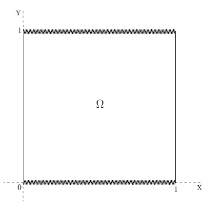
Example 15.

Let the domain of the solution space be $\mathrm{\Omega }\times (0,1]$, where $\mathrm{\Omega }$ denotes the square $(0,1)\times (0,1)$. Consider the initial-boundary value problem:

(31)

We validate the characteristics of the error estimates for the linearized backward Euler and Crank-Nicolson schemes presented in Theorem 11 and Theorem 14 for the problem (31). The degrees of freedom ${\vartheta }_H$ lies in ${\mathrm{\Omega }}^{\text{in}}$. So, the nodal values of the inner triangulation ${𝒯}_H^{\text{in}}$ corresponding to the domain ${\mathrm{\Omega }}^{\text{in}}$ is computed. We have discretized the domain space using the two-scale grid, $H$ being the coarse mesh size and $h$ being the fine mesh size and $h\ll H$. Also, $k$ is chosen as the time step for time discretization. In order to check the optimal order accuracy in space we take different time steps in both schemes, $k=H^2$ in Backward Euler scheme and $k=H$ in Crank-Nicolson scheme.

Let $i$ denote the number of iterations. For each iteration $i$, let $E_i$ denote the error which corresponds to $L^{\mathrm{\infty }}(L^2)$-norm and $H_i$ denote the coarse grid size. We calculate the ROC as follows

$\text{ROC}(E_i)={\displaystyle \frac{\log (E_{i+1}/E_i)}{\log (H_{i+1}/H_i)}}.$

We have computed the ROC for both the spatial grid size and time step size. Here, we have fixed the time discretizations as $N=2187$ to check the convergence w.r.t. space. Also, we fix space discretizations with 7728 degrees of freedom for checking the convergence with respect to the time. For convenience, we use the notation ${\text{CFE}}_{\text{error}}$ and ${\text{FE}}_{\text{error}}$ to denote the composite finite element errors and the finite element errors in the $L^{\mathrm{\infty }}(L^2)$-norm, respectively.

Tables 1 and 3 give the results for the Backward difference scheme and Crank-Nicolson scheme, respectively. It is shown that optimal order convergence is achieved. Tables 2 and 4 give the respective results from the calculations for the standard FEM.

${\vartheta }_{\text{d}}$	${\text{CFE}}_{\text{error}}$	ROC	$N$	${\text{CFE}}_{\text{error}}$	ROC
27	5.232520e-01	–	3	6.565751e-01	–
92	1.382621e-01	1.9201	9	1.697086e-01	1.9519
360	3.611840e-02	1.9366	27	4.480898e-02	1.9212
1280	9.291181e-03	1.9588	81	1.163433e-02	1.9454
2942	2.330536e-03	1.9952	243	2.981867e-03	1.9641
7728	5.840493e-04	1.9965	729	7.618697e-04	1.9686

Table 1. CFE error in $L^{\mathrm{\infty }}(L^2)$-norm for backward Euler method.

${\vartheta }_{\text{d}}$	${\text{FE}}_{\text{error}}$	ROC	$N$	${\text{FE}}_{\text{error}}$	ROC
39	7.792012e-01	–	3	5.938930e-01	–
141	2.054512e-01	1.9232	9	1.523725e-01	1.9626
520	5.314463e-02	1.9508	27	3.774357e-02	2.0133
1986	1.354841e-02	1.9718	81	9.341532e-03	2.0145
5225	3.360677e-03	2.0113	243	2.305467e-03	2.0186
18641	8.155538e-04	2.0429	729	5.691414e-04	2.0182

Table 2. FE error in $L^{\mathrm{\infty }}(L^2)$-norm for backward Euler method.

${\vartheta }_{\text{d}}$	${\text{CFE}}_{\text{error}}$	ROC	$N$	${\text{CFE}}_{\text{error}}$	ROC
27	3.722538e-01	–	3	6.831887e-01	–
92	9.928079e-02	1.9067	9	1.821319e-01	1.9073
360	2.620631e-02	1.9216	27	4.713870e-02	1.9500
1280	5.705062e-03	2.1996	81	1.227660e-02	1.9410
2942	1.464129e-03	1.9622	243	3.101874e-03	1.9847
7728	3.696528e-04	1.9858	729	7.648985e-04	2.0198

Table 3. CFE error in $L^{\mathrm{\infty }}(L^2)$-norm for Crank-Nicolson method.

${\vartheta }_{\text{d}}$	${\text{FE}}_{\text{error}}$	ROC	$N$	${\text{FE}}_{\text{error}}$	ROC
39	6.804915e-01	–	3	6.603572e-01	–
141	1.722587e-01	1.9820	9	1.730689e-01	1.9319
520	4.279390e-02	2.0091	27	4.363164e-02	1.9879
1986	1.082153e-02	1.9835	81	1.093364e-02	1.9966
5225	2.643653e-03	2.0333	243	2.699145e-03	2.0182
18641	6.526734e-04	2.0181	729	6.555613e-04	2.0417

Table 4. FE error in $L^{\mathrm{\infty }}(L^2)$-norm for Crank-Nicolson method.

From Tables 1 and 3 it is obvious that ROC is attained at lesser degrees of freedom as compared to that of Tables 2 and 4 respectively, which is very beneficial as the computational time and cost is very less for the CFE method. We establish that this is the advantage of the CFE method and it is more efficient.

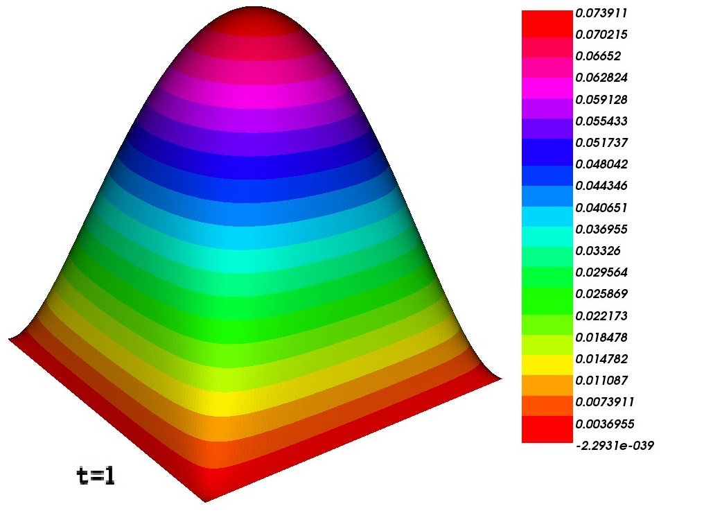
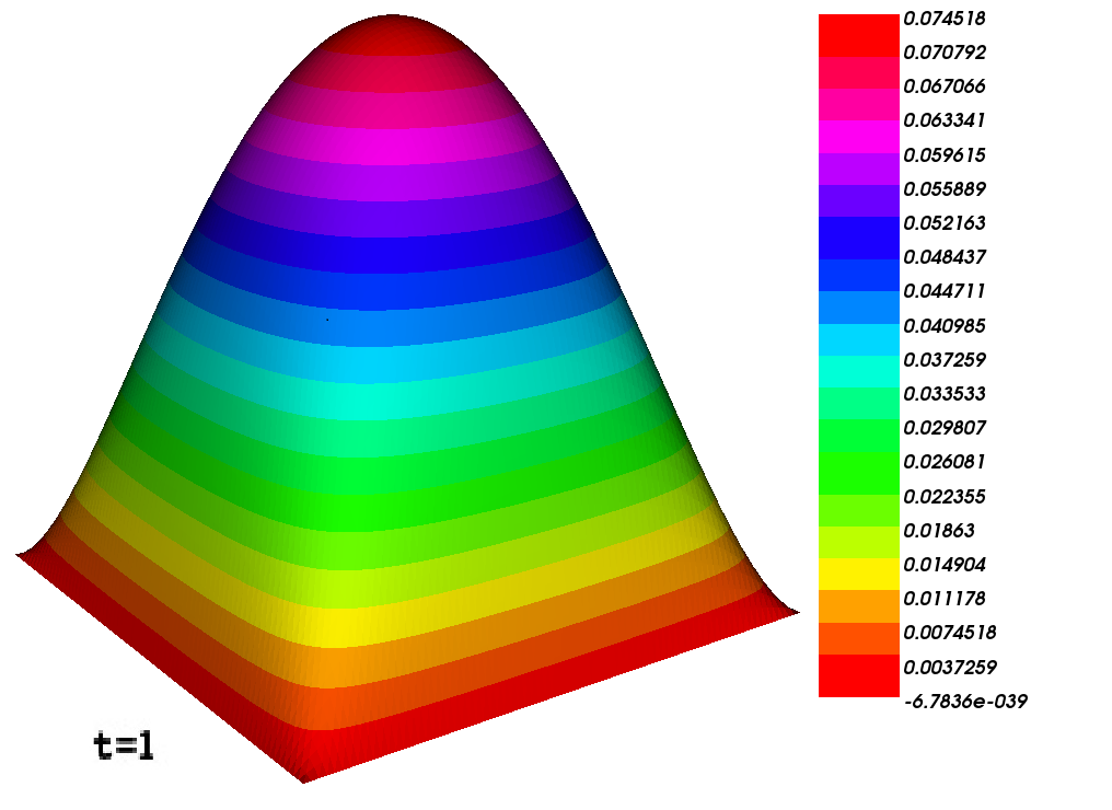
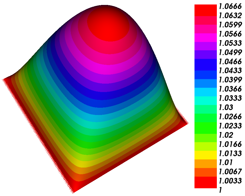
Now we consider the plots using the software FreeFEM++ and the results are given in respective figures. Fig. 4 demonstrates the CFE solution which is computed using the backward Euler method at the time level $t=1$ whereas Fig. 4 demonstrates the CFE solution computed using the Crank-Nicolson method.

Figure 3. CFE solution computed using the backward Euler method at the time level $t=1$.

Figure 4. CFE solution using the Crank-Nicolson method at the time level $t=1$.

Example 16.

Consider the following problem in $\mathrm{\Omega }$, which is now a computational domain with many geometric details. Assume that the domain $\mathrm{\Omega }$ is a zig-zag domain with 220 re-entering corners as shown in Fig. 6. Earlier the numerical experiments for linear model problem on zig-zag domain has been extensively studied, see e.g. [24]. In the present experiment, let us consider the model non-homogeneous problem as

(32)

Figure 5. Zig-zag domain having 220 re-entering corners.

Figure 6. CFE solution computed at the time level $t=0.5$ corresponding to the mesh sizes $H=0.015,h=0.009$ with the maximum value 1.0666.

Figure 7. Zoom view into boundary region (zig-zag segments) of the CFE solution depicted in Fig. 6.

Due to the presence of nonlinearity in $u$ on the right hand side, finding the analytical solution of the problem is highly challenging and hence we find the approximate solution numerically. Here we consider variable time step scheme. Let be a partition of the positive time axis and set $k_j=t_j-t_{j-1}$. Here we have chosen $t_0=0,t_1=0.07,t_2=0.16,t_3=0.24,t_4=0.33,t_5=0.43,t_6=0.5$ and the corresponding variable time step sizes are calculated as $k_1=0.07,k_2=0.09,k_3=0.08,k_4=0.09,k_5=0.1$ and $k_6=0.07$. Also let $U^n$ be the approximation of the exact solution given by $u(t_n)$, who values are calculated using the backward difference formula (22), where we have used the backward Euler quotient as ${\overline{\partial }}_n{U}^n=\frac{1}{k_n}(U^n-U^{n-1})$ for variable time steps. In this example we determine the CFE solution and the errors for the backward Euler method at every time level (cf. Table 5) and then obtain the $L^{\mathrm{\infty }}(L^2)$ errors and the corresponding ROC (cf. Table 6). The CFE solution is depicted in Fig. 6 and the zoom view of the solution is depicted in Fig. 7. From Table 6 one can observe that our scheme is providing an optimal order convergence which strongly supports our theoretical results.

$H$	$h$	Time level ($t$)	$u^{\text{CFE}}$	${\Vert u^{\text{CFE}}\left(t\right)-u\left(t\right)\Vert }_{L^2}$
0.12	0.072	0.07	0.96463	8.78541e-02
		0.16	0.97312	7.81550e-02
		0.24	0.98633	6.76764e-02
		0.33	0.98690	5.66721e-02
		0.43	1.06280	5.19924e-02
		0.50	1.06618	3.79710e-02
0.06	0.036	0.07	0.97039	2.49758e-02
		0.16	0.97539	2.00712 e-02
		0.24	0.98712	1.97321 e-02
		0.33	0.98792	1.71348 e-02
		0.43	1.06391	0.87562 e-02
		0.50	1.06642	0.68914 e-02
0.03	0.018	0.07	0.97507	6.91038e-03
		0.16	0.97719	6.04581e-03
		0.24	0.98781	4.88367e-03
		0.33	0.98996	3.88814e-03
		0.43	1.06445	2.66917e-03
		0.50	1.06653	2.00493e-03
0.015	0.009	0.07	0.98102	1.75991e-03
		0.16	0.98124	1.49616e-03
		0.24	0.99476	0.99715e-03
		0.33	0.99876	0.75984e-03
		0.43	1.06546	0.58582e-03
		0.50	1.06657	3.21776e-04

Table 5. CFE solution and error in different coarse-scale mesh sizes $H$ for varying time levels.

$H$	$h$	${\vartheta }_{\text{dof}}$	${\Vert u^{\text{CFE}}-u\Vert }_{L^{\mathrm{\infty }}\left(L^2\right)}$	ROC
0.12	0.072	42	8.78541e-02	–
0.06	0.036	141	2.49758e-02	1.8146
0.03	0.018	488	6.91038e-03	1.8537
0.015	0.009	1640	1.75991e-03	1.9733

Table 6. ROC in the $L^{\mathrm{\infty }}(L^2)$-norm.

7. Conclusion

In this paper we have put forward the idea of a variant of the finite element method, known as the composite finite element method. This is a two-scale method where we have two types of grids - coarse grid and fine grid. The primary benefit of the method is that the dimension depends on the coarser grids only, thereby reducing computational complexity. We considered the semilinear parabolic problem and derived the optimal order error estimates initially for the semidiscrete case and then for the fully discrete case. We have shown the theoretical proofs and, for validation, numerical experiments are carried out. We have used the backward Euler method and thereafter the Crank-Nicolson approach. We compared the obtained results with the standard FEM to show that the dimension of CFE space is much smaller than the standard FE space, which is very much beneficial. We have established that the proposed method gives efficient and optimal results.

Acknowledgements.

The authors would like to express their sincere thanks to the editor and the two anonymous referees for their helpful comments and suggestions, which have greatly improved the quality of this paper. The authors gratefully acknowledge valuable support provided by the Department of Mathematics, NIT Calicut and DST, Government of India, for providing support to carry out this work under the scheme ‘Faculty Research Grant (FRG)’ (No. FRG/2022/ MAT_01) and ‘FIST’ (No. SR/FST/MS-I/2019/40).

References

- [1] R.A. Adams, Sobolev Spaces, Academic Press, New York, 1975.
- [2] R.A. Adams, J.J. Fournier, Sobolev Spaces, Academic Press, 2003.
- [3] H. Amann, Existence and stability of solutions for semi-linear parabolic systems, and applications to some diffusion reaction equations, Proc. Roy. Soc. Edinburgh Sect. A, 81 (1978), pp. 35–47. https://doi.org/10.1017/S0308210500010428
- [4] A.K. Aziz, P. Monk, Continuous finite elements in space and time for the heat equation, Math. Comp., 52 (1989), pp. 255–274. https://doi.org/10.1090/S0025-5718-1989-0983310-2
- [5] J. Becker, A second order backward difference method with variable steps for a parabolic problem, BIT, 38 (2002), pp. 644–664. https://doi.org/10.1007/BF02510406
- [6] J.H. Bramble, Discrete methods for parabolic equations with time-dependent coefficients, Numer. Methods for PDE’s, Academic Press, 1979, pp. 41–52. https://doi.org/10.1016/B978-0-12-546050-7.50007-1
- [7] J.H. Bramble, P. Sammon, Efficient higher order single step methods for parabolic problems: Part I, Math. Comp., 35 (1980), pp. 655–677. https://doi.org/10.1090/S0025-5718-1980-0572848-X
- [8] P.G. Ciarlet, The Finite Element Method for Elliptic Problems, Class. Appl. Math., Society for Industrial and Applied Mathematics, Philadelphia, 2002. https://doi.org/10.1137/1.9780898719208
- [9] J. Douglas, Jr., T.F. Dupont, Galerkin methods for parabolic equations, SIAM J. Numer. Anal., 7 (1970), pp. 575–626. https://doi.org/10.1137/0707048
- [10] K. Eriksson, C. Johnson and V. Thomée, Time discretization of parabolic problems by the discontinuous Galerkin method, RAIRO Modél. Math. Anal. Numér., 19 (1985), pp. 611–643. https://doi.org/10.1051/m2an/1985190406111
- [11] D.J. Estep, M.G. Larson, R.D. Williams, Estimating the error of numerical solutions of reaction-diffusion equations, American Mathematical Soc., 146, No. 696, 2000. ?? https://doi.org/10.1090/memo/0696
- [12] W. Hackbusch and S.A. Sauter, Adaptive composite finite elements for the solution of PDEs containing nonuniformely distributed micro-scales, Mater. Model., 8 (1996) no. 9, pp. 31–43.
- [13] W. Hackbusch and S.A. Sauter, Composite finite elements for problems containing small geometric details. Part II: Implementation and numerical results, Comput. Vis. Sci., 1 (1997) no. 1, pp. 15–25. https://doi.org/10.1007/s007910050002
- [14] W. Hackbusch, S.A. Sauter, Composite finite elements for the approximation of PDEs on domains with complicated micro-structures, Numer. Math., 75 (1997) no. 4, pp. 447–472. https://doi.org/10.1007/s002110050248
- [15] D. Henry, Geometric Theory of Semilinear Parabolic Equations, Lecture Notes in Mathematics, 840, Springer, 2006.
- [16] H.-P. Helfrich, Error estimates for semidiscrete Galerkin type approximations to semilinear evolution equations with nonsmooth initial data, Numer. Math., 51 (1987) no. 5, pp. 559-569. https://doi.org/10.1007/BF01400356
- [17] P. Henry-Labordere, N. Oudjane, X. Tan, N. Touzi and X. Warin, Branching diffusion representation of semilinear PDEs and Monte Carlo approximation, Annales de l’Institut Henri Poincaré, Probabilités et Statistiques, 55 (2019) no. 1, pp. 184–210. https://doi.org/10.1214/17-AIHP880
- [18] M. Hutzenthaler, A. Jentzen, T. Kruse, T.A. Nguyen and P.V. Wurstemberger, Overcoming the curse of dimensionality in the numerical approximation of semilinear parabolic partial differential equations, Proc. R. Soc. A, Math. Phys. Eng. Sci., 476: 2244, 202), pp. 20190630. ?? https://doi.org/10.1098/rspa.2019.0630
- [19] M. Hutzenthaler, A. Jentzen, T. Kruse, Multilevel Picard iterations for solving smooth semilinear parabolic heat equations, Partial Differential Eq. Appl., 2 (2021) no. 6, pp. 1–31. https://doi.org/10.1007/s42985-021-00089-5
- [20] S. Larsson, Semilinear parabolic partial differential equations: thoery, approximation and applications, New Trends in the Mathematical and Computer Sciences, 3 (2006), pp. 153–194.
- [21] F. Liehr, T. Preusser, M. Rumpf, S. Sauter and L.O. Schwen, Composite finite elements for 3D image based computing, Comput. Visualization Sci. 12 (2009) no. 4, pp. 171–188. https://doi.org/10.1007/s00791-008-0093-1
- [22] T. Pramanick, R.K. Sinha, Two-scale composite finite element method for parabolic problems with smooth and nonsmooth initial data, J. Appl. Math. Comput., 58 (2018) nos. 1–2, pp. 469–501. https://doi.org/10.1007/s12190-017-1153-9
- [23] T. Pramanick and R.K. Sinha, Error estimates for two-scale composite finite element approximations of parabolic equations with measure data in time for convex and nonconvex polygonal domains, Appl. Numer. Math., 143 (2019), pp. 112–132. https://doi.org/10.1016/j.apnum.2019.03.009
- [24] T. Pramanick, R.K. Sinha, Composite finite element approximation for parabolic problems in nonconvex polygonal domains, Comp. Methods Appl. Math., 20 (2020) no. 2, pp. 361–378. https://doi.org/10.1515/cmam-2018-0155
- [25] M. Rech, Composite finite elements: An adaptive two-scale approach to the non-conforming approximation of Dirichlet problems on complicated domains, PhD thesis, Universität Zürich, 2006.
- [26] M. Rech, S.A. Sauter, A. Smolianski, Two-scale composite finite element method for Dirichlet problems on complicated domains, Numer. Math., 102 (2006) no. 4, pp. 681–708. https://doi.org/10.1007/s00211-005-0654-x
- [27] S. Sarraf, E.J. López, V.E. Sonzogni, M. B. Bergallo, An Algebraic Composite Finite Element Mesh Method, Cuadernos de Matemática y Mecánica, (2009).
- [28] S.A. Sauter, R. Warnke, Composite finite elements for elliptic boundary value problems with discontinuous coefficients, Computing, 77 (2006) no. 1, pp. 29–55. https://doi.org/10.1007/s00607-005-0150-2
- [29] V. Thomée, Galerkin Finite Element Methods for Parabolic Problems (Second Edition), Springer Ser. Comput. Math., Springer-Verlag, Berlin, 2006.
- [30] H. Triebel, Interpolation Theory, Function Spaces, Differential Operators, Johann Ambrosius Barth, Heidelberg, 1995.