The second order modulus revisited:
remarks, applications, problems

Abstract.

Several questions concerning the second order modulus of smoothness are addressed in this note. The central part is a refined analysis of a construction of certain smooth functions by Zhuk and its application to several problems in approximation theory, such as degree of approximation and the preservation of global smoothness. Lower bounds for some optimal constants introduced by Sendov are given as well. We also investigate an alternative approach using quadratic splines studied by Sendov.

1. Introduction

The present note could have likewise been called “Note on a paper by Zhuk” or “Note on a paper by Sendov”, which was also a preliminary title of this work. The point about this somewhat unusual introductory remark is that both Sendov and Zhuk have recently dealt (again) with certain natural questions concerning the classical second order modulus of continuity (denoted by $\left({\omega }_2\right)$ which have not yet been completely clarified. More precisely, the authors mentioned used different methods to construct smooth functions satisfying certain estimates in terms of ${\omega }_2$ and involving small constants. However, in spite of both authors’ interesting work and that of many others in the field, the question of best possible constants in inequalities of this type remains open. We take the liberty to cite from the paper [24] by Xin-long Zhou and the first author of this note, where it was stated that ${\omega }_2$ is a quantity which is not quite well understood yet. In the present paper we give refined analyses of the methods of Zhuk and Sendov, as well as a number of applications.

Let us first introduce some notation. For a compact interval , of the real axis we denote by $C[a,b]$ the space of all real-valued continuous functions on $[a,b]$, equipped with the usual sup norm given by ${\Vert f\Vert }_{C[a,b]}={\Vert f\Vert }_{\mathrm{\infty }}=\max \{\left|f\left(x\right)\right|:x\in [a,b]\}$. For $r\in \mathbb{N}$ we write

$$C^r[a,b]=\{f\in C[a,b]:f^{\left(r\right)}\in C[a,b]\},$$

and

$W_{r,\mathrm{\infty }}[a,b]=\{f\in C[a,b]:f^{\left(r-1\right)}$ is absolutely continuous with , where ${\Vert f\Vert }_{L_{\mathrm{\infty }}[a,b]}=$ $\parallel f\parallel L_{\mathrm{\infty }}=vraisup\{|f\left(x\right)|:x\in [a,b]\}.$

By ${\prod }_n[a,b],n\in \mathbb{N}\cup \{0\}$, we denote the linear space of algebraic polynomials of degree at most $n$. For $f\in C[a,b]$ and $[c,d]\subseteq [a,b]$, we write $E_n(f;[c,d])$ for the approximation constant of ${f|}_{[c,d]}$ with respect to ${\mathrm{\Pi }}_n[c,d]$. Special polynomials needed below will be $e_i,i\in \mathbb{N}\cup \{0\}$, the $i$-th monomials given by $e_i\left(x\right)=x_i$.

The problem discussed here essentially originated in a paper G. Freud [13]. In 1959 he proved a certain assertion which Brudnyĭ later generalized to the following theorem of utmost importance in approximation theory.

Theorem 1.1 (Brudnyĭ, [7, Proposition 2]).

Let $f\in C[0,1]$ and $s$ be a prescribed natural number. Then there exists a family of functions such that

(1) ${\Vert f-f_{s,h}\Vert }_{\mathrm{\infty }}$ $\le A_s{\omega }_s(f;h),$

(2) ${\Vert f_{s,h}^{\left(s\right)}\Vert }_{L_{\mathrm{\infty }}}$ $\le B_s{h}^{-s}{\omega }_s(f;h).$

Here ${\omega }_s$ denotes the (classical) $s$-th order modulus of continuity $it,e.g$, [27]), and the constants $A_s$ and $B_s$ depend only on $s$. Sometimes we shall write ${\omega }_s(f;h;[a,b])$ in order to explicitly indicate that the modulus is taken over the interval $[a,b]$. If we use the notation ${\omega }_s(f;h)$, this means that the modulus is taken over the interval of definition of the function $f$.

It is of interest to have information on the magnitude of the constants $A_s$ and $B_s$ figuring in the above theorem. There are two recent contributions by Zhuk [35] and Sendov [28] in which this problem is discussed from different points of view. In the present note we shall further discuss Zhuk’s approach, give lower bounds for the cases $s=1$ and $s=2$, and include a number of applications. Special emphasis will be on the case $s=2$. In the final section we also deal with Sendov’s approach, which is closely related to Freud’s paper mentioned earlier.

At several stages of this note, Bernstein polynomials over an interval $[a,b]$ will be used. For $n\in \mathbb{N},f\in C[a,b]$ and $x\in [a,b]$, these are given by

(3) $$B_n(f;x)=\frac{1}{{\left[b-a\right]}^n}\sum _{k=0}^{n}f\left(a+k\frac{b-a}{n}\right)\left(\genfrac{}{}{0pt}{}{n}{k}\right){\left(x-a\right)}^k{\left(b-x\right)}^{n-k},a\le x\le b.$$

As is well known, the polynomials $B_{n}f$ approximate the continuous function $f$ arbitrarily well, as $n\to \mathrm{\infty }$. Thus, for $n=n\left(\epsilon \right)$ large enough, we have for any $\epsilon >0$ given.

2. Further estimates for Zhuk’s functions

Let us first recall Zhuk’s approach to constructing his smoothing functions $S_h(f,\cdot )\left(=f_{2,h}(\cdot )\right)\in W_{2,\mathrm{\infty }}[a,b]$.

For $f\in C[a,b]$, define first the extension

$$f_h:[a-h,b+h]\to ℝ$$

by

Here ${\Vert f-P_{-}\Vert }_{C[a,a+2h]}=E_1(f;a,a+2h)$, and ${\Vert f-P_{+}\Vert }_{C[b-2h,b]}=E_1(f;b-2h,b)$, i.e., $P_{-},P_{+}\in$ ${\prod }_1$are the best approximations to $f$ on the intervals indicated.

Then Zhuk defined the second order Steklov means

$$S_h(f,x):=\frac{1}{h}\cdot {\int }_{-h}^h\left(1-\frac{\left|t\right|}{h}\right)f_h\left(x+t\right)𝑑t,x\in [a,b],$$

and showed the following

Lemma 2.1 ([35, Lemma 1]).

Let . Then

• ${\Vert f-S_h(f;\cdot )\Vert }_{C[a,b]}\le \frac{3}{4}\cdot {\omega }_2(f;h),$

• ${\Vert {\left(S_{h}f\right)}^{\prime \prime }\Vert }_{L_{\mathrm{\infty }}[a,b]}\le \frac{3}{2}\cdot h^{-2}\cdot {\omega }_2(f;h).$

In the next lemma we show that there is a pointwise refinement of Lemma 2.1 $\left(i\right)$ in the sense that in the middle of the interval the constant 3/4 can be decreased. For the sake of simplicity we treat only the cases $[a,b]=[0,1]$. The pointwise improvement reads as follows.

Lemma 2.2.

Let and let $S_h(f,\cdot )$ be given as above. Then

Proof.

We first rewrite $S_h(f,x)$ as follows:

$S_h(f;x)$ $=\frac{1}{h}\cdot \left[{\displaystyle {\int }_0^h}\left(f-\frac{t}{h}\right)\cdot f_h\left(x+t\right)𝑑t-{\displaystyle {\int }_h^0}\left(1-\frac{t}{h}\right)\cdot f_h\left(x-t\right)𝑑t\right]$

$=\frac{1}{h^2}\cdot {\displaystyle {\int }_0^h}\left(h-t\right)\cdot \left(f_h\left(x+t\right)+f_h\left(x-t\right)\right)𝑑t.$

Let $x\in [h,1-h],h\le \frac{1}{2}$. Then for $t\in [0,h],h\le x+t\le 1$ and $0\le x-t\le 1-h$, i.e., $x\pm t\in [0,1]$.

Hence

$$S_h(f;x)=\frac{1}{h^2}\cdot {\int }_0^h\left(h-t\right)\cdot \left(f\left(x+t\right)+f\left(x-t\right)\right)𝑑t.$$

Since

$$\frac{1}{h^2}\cdot {\int }_0^h\left(h-t\right)𝑑t=\frac{1}{2},$$

we have

$\left|S_h(f;x)-f\left(x\right)\right|$ $=\left|\frac{1}{h^2}\cdot {\displaystyle {\int }_0^h}\left(h-t\right)\left(f\left(x+t\right)-2f\left(x\right)+f\left(x-t\right)\right)𝑑t\right|$

$\le \frac{1}{h^2}\cdot {\displaystyle {\int }_0^h}\left(h-t\right)\cdot {\omega }^2(f;t)𝑑t$

$\le \frac{1}{h^2}\cdot {\displaystyle {\int }_0^h}\left(h-t\right)𝑑t\cdot {\omega }_2(f;h)=dt\frac{1}{2}.{\omega }_2(f;h).$

Let . Then $x+t\in [0,2h]$ and $x-t\in [-h,h]$, if $t\in [0,h]$.

In this case,

$S_h(f;x)\frac{1}{h^2}\cdot {\displaystyle {\int }_0^h}\left(h-t\right)\cdot \left(f\left(x+t\right)+f_h\left(x-t\right)\right)𝑑t=$

$=\frac{1}{h^2}\cdot \left({\displaystyle {\int }_0^x}+{\displaystyle {\int }_x^h}\right)\left(h-t\right)\cdot \left(f\left(x+t\right)+f_h\left(x-t\right)\right)dt$

$=\frac{1}{h^2}\cdot \{{\displaystyle {\int }_0^x}(h-t)\cdot (f(x+t)+f(x-t))dt$

$+{\displaystyle {\int }_x^h}(h-t)\cdot (f(x+t)+P_{-}(x-t))dt\}.$

This implies

$\left|S_h(f;x)-f\left(x\right)\right|$ $=|\frac{1}{h^2}\cdot \{{\displaystyle {\int }_0^x}(h-t)(f(x+t)-2f\left(x\right)+f(x-t))dt$

$+{\displaystyle {\int }_x^h}(t-t)\cdot (f(x+t)-2f\left(x\right)+P_{-}(x-t))dt\left\}\right|$

$\le \frac{1}{h^2}\cdot {\displaystyle {\int }_0^x}\left(h-t\right)\cdot {\omega }_2(f;t)𝑑t$

$+\frac{1}{h^2}\cdot {\displaystyle {\int }_x^h}\left(h-t\right)\cdot \left|f\left(x+t\right)-2f\left(x\right)+P_{-}\left(x-t\right)\right|𝑑t.$

Here we have

$\left|f\left(x+t\right)-2f\left(x\right)+P_{-}\left(x-t\right)\right|\le$

$\le \left|P_{-}\left(x-t\right)-2P_{-}\left(x\right)+P_{-}\left(x+t\right)\right|$

$+2\cdot \left|P_{-}\left(x\right)-f\left(x\right)\right|+\left|P_{-}\left(x+t\right)-f\left(x+t\right)\right|.$

Since $P_{-}\in {\prod }_1,\left|P_{-}\left(x-t\right)-2P_{-}\left(x\right)+P_{-}\left(x+t\right)\right|=0$.

For the remaining two differences we have, for, $y\in \{x,x+t\}\subset [0,2h]$,

$$\left|P_{-}\left(y\right)-f\left(y\right)\right|\le \frac{1}{2}\cdot {\omega }_2(f;h).$$

The latter inequality follows from the second part of the following lemma due to Burkill [8, Lemma 5.2] and Whitney [33]. See also [29] or [30, Lemma 2.3], and [3] for the first part and [35, Lemma 1], proof of for the second one. The first part will be used later on. ∎

Lemma 2.3.

For a compact interval $[\alpha ,\beta ]$ and $f\in C[\alpha ,\beta ]$, the following are true:

• If $\mathrm{\ell }$ denotes the linear function interpolating $f$ af $\alpha$ and $\beta$, then

  $$\left|f\left(x\right)-\mathrm{\ell }\left(x\right)\right|\le {\omega }_2(f;\frac{\beta -\alpha }{2})\text{ for all }x\in [\alpha ,\beta ].$$

• If $P_1$ is the best approximation to $f$ by elements of ${\prod }_1$, then

  $$\left|f\left(x\right)-P_1\left(x\right)\right|\le \frac{1}{2}\cdot {\omega }_2(f;\frac{\beta -\alpha }{2})\text{ for all }x\in [\alpha ,\beta ].$$

Proof of Lemma 2.2 (cont’d): Hence for $0\le x\le h$,

$\left|S_h(f;x)-f\left(x\right)\right|$ $\le \frac{1}{h^2}{\displaystyle {\int }_0^x}\left(h-t\right){\omega }_2(f;t)𝑑t+\frac{1}{h^2}{\displaystyle {\int }_x^h}\left(h-t\right)\frac{3}{2}{\omega }_2(f;h)𝑑t$

$\le \frac{1}{h^2}{\displaystyle {\int }_0^x}\left(h-t\right){\omega }_2(f;h)𝑑t+\frac{1}{h^2}{\displaystyle {\int }_x^h}\left(h-t\right)\frac{3}{2}{\omega }_2(f;h)𝑑t$

$=\frac{1}{h^2}{\omega }_2(f;h)\left({\displaystyle {\int }_0^x}\left(h-t\right)𝑑t+{\displaystyle {\int }_x^h}\frac{3}{2}\left(h-t\right)𝑑t\right).$

Here

$${\int }_0^x\left(h-t\right)𝑑t+\frac{3}{2}{\int }_x^h\left(h-t\right)𝑑t=\frac{1}{2}{h}^2+\frac{1}{4}{\left(h-x\right)}^2,$$

giving the desired inequality for . The remaining case can  be treated analogously to the first one, and thus the proof is complete.

As can be seen from the example below (see Section 4 in particular), it is sometimes convenient to have estimates for lower order derivatives of $S_{h}f$ available as well. See [21] for another situation in which such estimates are useful. In the following lemma we supplement the estimates from Lemmas 2.1 and 2.2 in this sense. Cf. Lemma 2.2 in [20], where similar inequalities for second order Steklov means were given (based upon different extensions of $f$, however).

Lemma 2.4.

Let $f,h$ and $S_{h}f$ be given as in Lemma 2.1 Then

$$\parallel S_{h}f){}^{\prime }\parallel {}_{C[a,b]}\le \frac{1}{4}[2\cdot {\omega }_1(f;h)+\frac{3}{2}\cdot {\omega }_2(f;h)],$$

and

$${\Vert S_{h}f\Vert }_{C[a,b]}\le {\Vert f\Vert }_{C[a,b]}+\frac{3}{4}\cdot {\omega }_2(f;h).$$

Proof.

The second inequality is a simple consequence of

$${\Vert f-S_{h}f\Vert }_{C[a,b]}\le \frac{3}{4}\cdot {\omega }_2(f;h),$$

which implies

$${\Vert S_{h}f\Vert }_{C[a,b]}\le {\Vert f\Vert }_{C[a,b]}+\frac{3}{4}\cdot {\omega }_2(f;h).$$

The first inequality is obtained as follows. Write

$S_h(f;x)$ $=h^{-1}\cdot \left[{\displaystyle {\int }_0^h}\left(1-\frac{t}{h}\right)f_h\left(x+t\right)𝑑t+{\displaystyle {\int }_{-h}^0}\left(1+\frac{t}{h}\right)f_h\left(x+t\right)𝑑t\right]$

$=h^{-1}\cdot \left[{\displaystyle {\int }_0^h}\left(1-\frac{t}{h}\right)f_h\left(x+t\right)𝑑t+{\displaystyle {\int }_0^h}\left(1+\frac{t}{h}\right)\cdot f_h\left(x-t\right)𝑑t\right].$

Here,

$${\int }_0^h\left(1-\frac{t}{h}\right)\cdot f_h\left(x+t\right)𝑑t=-F\left(x\right)+\frac{1}{h}\cdot {\int }_0^{h}F\left(x+t\right)𝑑t,$$

where $F$ is an antiderivative of $f_h$.

Likewise,

$${\int }_0^h\left(1-\frac{t}{h}\right)\cdot f_h\left(x-t\right)𝑑t=F\left(x\right)-\frac{1}{h}{\int }_0^{h}F\left(x-t\right)𝑑t.$$

Hence,

$$S_h(f;x)=\frac{1}{h^2}{\int }_0^h\left[F\left(x+t\right)-F\left(x-t\right)\right]𝑑t$$

which implies

${\left(S_{h}f\right)}^{\prime }\left(x\right)$ $=\frac{1}{h^2}\cdot {\displaystyle {\int }_0^h}\left[f_h\left(x+t\right)-f_h\left(x-t\right)\right]𝑑t$

$=\frac{1}{h^2}\cdot h\cdot \left[f_h\left(x+\xi \right)-f_h\left(x-\xi \right)\right],0\le \xi \le h$

(differentiation under the integral, mean value theorem).

In order to estimate $\left|{\left(S_{h}f\right)}^{\prime }\left(x\right)\right|$, it remains to estimate $\left|f_h\left(x+\xi \right)-f_h\left(x-\xi \right)\right|$. Suppose first that $x+\xi ,x-\xi \in [a,b]$.

Then

$\left|f_h\left(x+\xi \right)-f_h\left(x-\xi \right)\right|$ $=\left|f\left(x+\xi \right)-f\left(x-\xi \right)\right|\le {\omega }_1(f;2\xi )\le 2\cdot {\omega }_1(f;h).$

Now assume that

Then $f_h\left(x-\xi \right)=P_{-}\left(x-\xi \right)$ so that

$\left|f_h\left(x+\xi \right)-f_h\left(x-\xi \right)\right|=\left|f\left(x+\xi \right)-f\left(x\right)+f\left(x\right)-P_{-}\left(x\right)+P_{-}\left(x\right)-P_{-}\left(x-\xi \right)\right|.$

Due to the linearity of $P_{-}$, we have $P_{-}\left(x\right)-P_{-}\left(x-\xi \right)=P_{-}\left(x+\xi \right)-P_{-}\left(x\right)$. Using this, we get

$\left|f_h\left(x+\xi \right)-f_h\left(x-\xi \right)\right|\le \left|f\left(x+\xi \right)-f\left(x\right)\right|+\left|f\left(x\right)-P_{-}\left(x\right)\right|$

$+\left|P_{-}\left(x+\xi \right)-f\left(x+\xi \right)\right|+\left|f\left(x+\xi \right)-f\left(x\right)\right|+\left|f\left(x\right)-P_{-}\left(x\right)\right|.$

As we know from Lemma 2.3 on the interval $[a,\alpha +2h]$ one has

$$\left|f\left(y\right)-P_{-}\left(y\right)\right|\le \frac{1}{2}\cdot {\omega }_2(f;h;[a,\alpha +2h])\le \frac{1}{2}\cdot {\omega }_2(f;h;[a,b]).$$

Hence it follows that

$\left|f_h\left(x+\xi \right)-f_h\left(x-\xi \right)\right|\le$

$\le {\omega }_1(f;h)+\frac{1}{2}\cdot {\omega }_2(f;h)+\frac{1}{2}\cdot {\omega }_2(f;h)+{\omega }_1(f;h)+\frac{1}{2}\cdot {\omega }_2(f;h)$

$=2\cdot {\omega }_1(f;h)+\frac{3}{2}\cdot {\omega }_2(f;h).$

The remaining case, namely

can be treated analogously to the second one. ∎

Corollary 2.5.

As an immediate consequence of Lemma 2.4 one has the simpler inequalities

$${\Vert {\left(S_{h}f\right)}^{\prime }\Vert }_{C[a,b]}\le \frac{5}{h}\cdot {\omega }_1(f;h),\text{ and }{\Vert S_{h}f\Vert }_{C[a,b]}\le 4\cdot {\Vert f\Vert }_{C[a,b]}$$

Corollary 2.6.

However, for assertions in  which small constants are of interest in the final statement, it is not advisable to use the latter inequalities.

3. Lower bounds for $A_S^{\ast },s=1,2.$

It was shown by Sendov [28, p. 198] that the constant $B_s$ in Brudnyĭ’s theorem can never be less than one. This motivates the following.

Definition 3.1.

We denote by $A_S^{\ast }\left(B_S\right)$ the smallest number (provided it exists) for which Brudnyĭ’s Theorem 1.1 holds for a given $B_S\ge 1$ and $A_S^{\ast }\left(B_S\right)$.

Very little is known about the funciton $A_S^{\ast }\left(B_S\right)$, even for the cases $s=1$ and $s=2$. Let us first recall a result from Sendov’s paper. He showed that it is possible to have $B_1=1$, and that $A_1^{\ast }\left(B_1\right)\le 1$. This is supplemented by the following assertion in which we give a lower bound for $A_1^{\ast }\left(B_1\right)$.

Theorem 3.2.

$$A_1^{\ast }\left(1\right)\ge \frac{1}{2}.$$

Proof.

Let $f\in C[0,1]$ be arbitrary. Choose the family such that

$${\Vert f-f_h\Vert }_{\mathrm{\infty }}\le A_1^{\ast }(1)\cdot {\omega }_1(f;h),$$

and

$${\Vert f_h^{\prime }\Vert }_{L\mathrm{\infty }}\le 1;h^{-1}\cdot {\omega }_1(f;h).$$

Now consider the Bernstein polynomials $B_{n}f$. One has, for any $g\in W_{1,\mathrm{\infty }}[0,1]$,

${\omega }_1(B_{n}f;h)$ $\le {\omega }_1[B_n\left(f-g\right);h]+{\omega }_1(B_{n}g;h)$

$\le 2\cdot \Vert B_n\Vert \cdot {\Vert f-h\Vert }_{\mathrm{\infty }}+{\Vert {\left(B_{n}g\right)}^{\prime }\Vert }_{\mathrm{\infty }}\cdot h\le 2\cdot {\Vert f-g\Vert }_{\mathrm{\infty }}+{\Vert g^{\prime }\Vert }_{L_{\mathrm{\infty }}}\cdot h.$

Choosing $g=f_n$ gives

${\omega }_1(B_{n}f;h)$ $\le 2\cdot A_1^{\ast }\left(1\right)\cdot {\omega }_1(f;h)+{\omega }_1(f;h)$

It was shown in [2] (see Remark (ii) following Theorem 9 there) that the inequality

can hold only if $c\ge 2$. Hence $2\cdot A_1^{\ast }\left(1\right)+1\ge 2,$ or $A_1^{\ast }\left(1\right)\ge 1/2$.

We consider the case $s=2$. The result of Zhuk from Lemma 2.1 can be rephrased by saying that $A_2^{\ast }\left(3/2\right)\le 3/4$. A lower bound is given in ∎

Theorem 3.3.

$$A_2^{\ast }\frac{3}{2}\ge \frac{13}{32}.$$

Proof.

A query published in the proceedings of the 1982 Edmonton Conference on approximation theory (see [19] and Example 4.13 (ii) below) contains the information that it was known then that

(4) $$1\le \underset{n\in \mathbb{N}}{sup}\underset{\begin{array}{c}f\in C[0,1]\\ f\ne linear\end{array}}{sup}\frac{{\Vert B_{n}f-f\Vert }_{\mathrm{\infty }}}{{\omega }_2(f;\frac{1}{\sqrt{n}})}.$$

The same fact was also observed by Păltănea in 1990, see [26, Theorem 3.2]. This means that

$${\Vert B_{n}f-f\Vert }_{\mathrm{\infty }}\le c\cdot {\omega }_2(f;\frac{1}{\sqrt{n}}),n\in \mathbb{N},f\in C[0,1],$$

cannot hold for any constant .

For the Bernstein operators we have, for any $f\in C[0,1],g\in W_{2,\mathrm{\infty }}[0,1]$,

${\Vert B_{n}f-f\Vert }_{\mathrm{\infty }}$ ${\Vert B_n\left(f-g\right)-\left(f-g\right)\Vert }_{\mathrm{\infty }}+{\Vert B_{n}g-g\Vert }_{\mathrm{\infty }}\le$

$\le 2\cdot {\Vert f-g\Vert }_{\mathrm{\infty }}+\frac{1}{8n}\cdot {\Vert g^{\prime \prime }\Vert }_{L_{\mathrm{\infty }}}$

(cf. [11], p. 40]).

Now let $f_n$ be functions with

$${\Vert f_h^{\prime \prime }\Vert }_{L_{\mathrm{\infty }}}\le \frac{3}{2}{h}^{-2}\cdot {\omega }_2(f;h),$$

and

Choose $g=f_h$ with $h=\frac{1}{\sqrt{n}}$. This gives

${\Vert B_{n}f-f\Vert }_{\mathrm{\infty }}$ $\le 2\cdot \Vert f-f_h\Vert +\frac{1}{8}\cdot \frac{1}{n}\cdot \Vert f_h^{\prime \prime }\Vert$

$\le 2\cdot A_2^{\ast }\left(\frac{3}{2}\right)\cdot {\omega }_2(f;\frac{1}{\sqrt{n}})+\frac{3}{2}\cdot \frac{1}{8}\cdot \frac{1}{n}\cdot n\cdot {\omega }_2(f;\frac{1}{\sqrt{n}})$

$=\left(2\cdot A_2^{\ast }\left(\frac{3}{2}\right)+\frac{3}{16}\right)\cdot {\omega }_2(f;\frac{1}{\sqrt{n}}).$

From (4), we know that $2\cdot A_2^{\ast }\left(\frac{3}{2}\right)+\frac{3}{16}\ge 1$, i.e.,$A_2^{\ast }\left(\frac{3}{2}\right)\ge \frac{13}{32}$. ∎

Remark 3.4.

The lower bound $1$ used in the proof of Theorem 3.3 was derived early in 1982 by the first author. It served as the motivation for a joint project with his former student Hans Kessler during the winter and spring terms of 1982 at Rensselaer Polytechnic Institute in which we tried to find a function $f_0$ with

$${\Vert B_n{f}_0-f_0\Vert }_{\mathrm{\infty }}>{\omega }_2(f_0;\frac{1}{\sqrt{n}})$$

for some natural $n$.

The numerical experiments then carried our failed to produce such a function. This experience, together with the then-known inequality.

$$\underset{n\in \mathbb{N}}{sup}\underset{\begin{array}{c}f\in C[0,1]\\ f\ne linear\end{array}}{sup}\frac{{\Vert B_{n}f-f\Vert }_{\mathrm{\infty }}}{{\omega }_2\cdot (f;\frac{1}{\sqrt{n}})}\le 3.25,$$

led us to publish the query in the Alberta conference proceedings of 1982 mentioned earlier.

4. Applications

In this section we give a collection of applications of the inequalities in Section 2. At several stages we critically discuss the power of the general estimates derived here by comparing them with results obtained in some special situations.

4.1. General Operators

In the following lemma we show that functions in $W_{2,\mathrm{\infty }}[a,b]$ can be approximated arbitrarily well by functions in $C^2[a,b]$, while retaining important differential characteristics. In fact, Bernstein polynomials do the job quite well as will be seen from the proof of the lemma. The main purpose in including it, however, is to be able to give a simple proof of the subsequent Theorem 4.2 , which is one of the key results of this section.

Lemma 4.1.

For each $g\in W_{2,\mathrm{\infty }}[a,b]$ and $\epsilon >0$, there is a polynomial $p=p(g,\epsilon )$ such that

• and

• $${\Vert p^{\prime \prime }\Vert }_{\mathrm{\infty }}\le {\Vert g^{\prime \prime }\Vert }_{L_{\mathrm{\infty }}[a,b]}.$$

Proof.

For $g\in W_{2,\mathrm{\infty }}[a,b]$, choose $p=B_{n}g$, with $n$ large enough to have . For the $k$-th derivative of $B_{n}g$ one has, for $0\le k\le n$, the representation

$${\left(B_{n}g\right)}^{\left(k\right)}\left(x\right)=\frac{n\mathrm{\dots }\left(n-k+1\right)}{{\left(b-a\right)}^n}\sum _{i=0}^{n-k}{\mathrm{△}}^{i}g\left(a+\frac{i\left(b-a\right)}{n}\right)\left(\genfrac{}{}{0pt}{}{n-k}{i}\right){\left(x-a\right)}^i{\left(b-x\right)}^{n-k-i},$$

where ${\mathrm{△}}^i$is an $i$-th order forward difference with stepsize $\frac{b-a}{n}$.

The case $k=0$ immediately shows ${\Vert p\Vert }_{\mathrm{\infty }}\le {\Vert g\Vert }_{\mathrm{\infty }}$.

For $k=1$ we have

$${\left(B_{n}g\right)}^{\prime }\left(x\right)=\frac{n}{{\left(b-a\right)}^n}\sum _{i=0}^{n-1}{\mathrm{△}}^{\prime }g\left(a+\frac{i\left(b-a\right)}{n}\right)\left(\genfrac{}{}{0pt}{}{n-1}{i}\right){\left(x-a\right)}^i{\left(b-x\right)}^{n-1-i}$$

Here

$$\left|{\mathrm{△}}^{1}g\left(x\right)\right|=g\left(x\right)-g\left(x+\frac{b-a}{n}\right)\le {\Vert g^{\prime }\Vert }_{\mathrm{\infty }}\frac{b-a}{n}\text{.}$$

Hence

$${\Vert {\left(B_{n}g\right)}^{\prime }\Vert }_{\mathrm{\infty }}\le \frac{n}{{\left(b-a\right)}^n}\cdot {\Vert g^{\prime }\Vert }_{\mathrm{\infty }}\frac{b-a}{n}{\left(b-a\right)}^{n-1}={\Vert g^{\prime }\Vert }_{\mathrm{\infty }}.$$

For the second derivative one has

${\left(B_{n}g\right)}^{\prime \prime }\left(x\right)=\frac{n\left(n-1\right)}{{\left(b-a\right)}^n}\cdot {\displaystyle \sum _{i=0}^{n-2}}{\mathrm{△}}^{2}g\left(a+\frac{i\left(b-a\right)}{n}\right)\left(\genfrac{}{}{0pt}{}{n-2}{i}\right){\left(x-a\right)}^i{\left(b-x\right)}^{n-i-2},$

where

$\left|{\mathrm{△}}^{2}g\left(x\right)\right|$ $=\left|g\left(x\right)-2g\left(x+\frac{b-a}{n}+g\right)\left(x+2\frac{b-a}{n}\right)\right|=$

$=\left|{\mathrm{△}}^{1}g\left(x+\frac{b-a}{n}\right)-{\mathrm{△}}^{1}g\left(x\right)\right|$

$=\left|{\left({\mathrm{△}}^{1}g\right)}^{\prime }\left({\xi }_1\right)\frac{b-a}{n}\right|\text{ with }{\xi }_1\in (x,x+\frac{b-a}{n})$

$=\left|\frac{b-a}{n}{\displaystyle {\int }_{{\xi }_1}^{{\xi }_1+\frac{b-a}{n}}}{g}^{\prime \prime }\left(t\right)𝑑t\right|\text{(}{g}^{\prime }\text{ absolutely continuous)}$

$\le {\left(\frac{b-a}{n}\right)}^2\cdot {\Vert g^{\prime \prime }\Vert }_{L_{\mathrm{\infty }}}.$

∎

This implies $\left|{\left(B_{n}g\right)}^{\prime \prime }\left(x\right)\right|\le {\Vert g^{\prime \prime }\Vert }_{L_{\mathrm{\infty }}}$, which concludes the proof of the lemma.

Using Lemma 4.1 and the results from Section 2 , we present next a partial generalization of another theorem of Brudnyĭ (see [7, Theorem 9]), which is more appropriate for application purposes than earlier contributions by other authors. As far as earlier work is concerned, particularly for the case of linear operators, that of Freud [13, Main theorem] and Stečkin [32, Theorem 5], must be mentioned. For this so-called smoothing technique, see also [12, Theorems 2.2 through 2.4]. While we restrict ourselves here to the case of ${\omega }_2$, the analogous problems still exist for the cases of ${\omega }_k,k\ge 3$. Our generalization of Brudnyĭ’s result reads as follows.

Theorem 4.2.

Let $(B\parallel \cdot {\parallel }_B)$ be a Banach space, and let $H:C[a,b]\to (B,\parallel \cdot {\parallel }_B)$ be an operator, where

• $${\Vert H\left(f+g\right)\Vert }_B\le \gamma \cdot \{{\Vert Hf\Vert }_B+{\Vert Hg\Vert }_B\}\text{ for all }f,g\in C[a,b];$$

• $${\Vert Hf\Vert }_B\le \alpha \cdot {\Vert f\Vert }_C\text{ for all }f\in C[a,b];$$

• $${\Vert Hg\Vert }_B\le {\beta }_0\cdot {\Vert g\Vert }_C+{\beta }_1\cdot {\Vert g^{\prime }\Vert }_C+{\beta }_2\cdot {\Vert g^{\prime \prime }\Vert }_C\text{ for all }g\in C^2[a,b].$$

Then for all , the following inequality holds:

${\Vert Hf\Vert }_B\le \gamma \cdot \{{\beta }_0\Vert f\parallel +\frac{2{\beta }_1}{h}\cdot {\omega }_1(f;h)+\frac{3}{4}\left(\alpha +{\beta }_0+\frac{2{\beta }_1}{h}+\frac{2{\beta }_2}{h^2}\right)\cdot {\omega }_2(f;h)\}.$

Proof.

For arbitrary $\overline{g}\in W_{2,\mathrm{\infty }}[a,b],g\in C^2[a,b]$, we have

${\Vert Hf\Vert }_B$ $={\Vert H\left(f-\overline{g}+\overline{g}-g+g\right)\Vert }_B$

$\le \gamma \cdot \left\{{\Vert H\left(f-\overline{g}+\overline{g}-g\right)\Vert }_B+{\Vert Hg\Vert }_B\right\}$

$\le \gamma \cdot \left\{\alpha \cdot {\Vert f-\overline{g}+\overline{g}-g\Vert }_C+{\beta }_0\cdot {\Vert g\Vert }_C+{\beta }_1\cdot {\Vert g^{\prime }\Vert }_C+{\beta }_2\cdot {\Vert g^{\prime \prime }\Vert }_C\right\}$

$\le \gamma \cdot \left\{\alpha \cdot {\Vert f-\overline{g}\Vert }_C+\alpha \cdot {\Vert \overline{g}-g\Vert }_C+{\beta }_0\cdot {\Vert g\Vert }_C+B_1\cdot {\Vert g^{\prime }\Vert }_C+{\beta }_2\cdot {\Vert g^{\prime \prime }\Vert }_C\right\}.$

For , now choose $\overline{g}=S_{h}f$. This implies

${\Vert Hf\Vert }_B\le \gamma \cdot \{\alpha \cdot \frac{3}{4}\cdot {\omega }_2(f;h)+\alpha \cdot {\Vert S_{h}f-g\Vert }_C+{\beta }_0\cdot {\Vert g\Vert }_C+{\beta }_1{\Vert g^{\prime }\Vert }_C+{\beta }_2\cdot {\Vert g^{\prime \prime }\Vert }_C\}.$

For arbitrary $\omega >0$, replace $g$ by the polynomial $p=p(S_{h}f,\epsilon )$ from Lemma 4.1 This yields the estimate

${\Vert Hf\Vert }_B$ $\le \gamma \cdot \{\alpha \cdot \frac{3}{4}\cdot {\omega }_2(f;h).+\alpha \cdot \epsilon +{\beta }_0\cdot \parallel S_{h}f{\parallel }_C+{\beta }_1\cdot \parallel {\left(S_{h}f\right)}^{\prime }{\parallel }_C+{\beta }_2\cdot \parallel {\left(S_{h}f\right)}^{\prime \prime }{\parallel }_{L_{\mathrm{\infty }}}\}$

$\le \gamma \cdot \{\alpha \cdot \frac{3}{4}\cdot {\omega }_2(f;h)+\alpha \cdot \epsilon +{\beta }_0\cdot (\parallel f\parallel +\frac{3}{4}\cdot {\omega }_2(f;h))$

$+{\beta }_1\cdot (\frac{2}{h}\cdot {\omega }_1(f;h)+\frac{3}{2h}{\omega }_2(f;h))+{\beta }_2\cdot \frac{3}{2}\cdot \frac{1}{h^2}\cdot {\omega }_2(f;h)\}.$

In the latter estimate we have used Lemma 2.1 and Lemma 2.4 Letting $\epsilon$ tend to zero the desired inequality. ∎

Corollary 4.3.

In many cases one has $\gamma =1$ and ${\beta }_0={\beta }_1=0$, so that the inequality from Theorem 4.2 simplifies to

$${\Vert Hf\Vert }_B\le \left(\frac{3\alpha }{4}+\frac{3{\beta }_2}{2\cdot h^2}\right)\cdot {\omega }_2(f;h).$$

Remark 4.4.

The constants $\frac{3}{4}$ and $\frac{3}{2}$ figuring in Corollary 4.3 are probably not best possible. Note that they arise exclusively from the choice of the smoothing functions $S_{h}f$, and thus depend on each orther. More sophisticated choices of $S_{h}f$ might lead to an improved result.

Remark 4.5.

• If $H$ is linear, then condition a) of Theorem 4.2 is automatically fulfilled with $\gamma =1$.

• Typical examples of non-linear operators $H$ satisfying the assumptions of Theorem 4.2 are those of the from ${\omega }_2(L(\cdot );\delta )$, where $k\in {\mathbb{N}}_0$, and the linear operator $L$ and $\delta \ge 0$ are fixed.

• Instances of linear operators $H$ satisfying the assumptions of Theorem 4.2 are given by, e.g.,${\epsilon }_x\cdot L$, where ${\epsilon }_X$ is a point-evaluation functional and $L$ is some linear operator.

4.1.1. 4.2.Examples (non-linear case)

Global Smoothness Preservation

As a first application of Theorem 4.2 (or Corollary 4.3, inequality concerning the preservation of global smoothness by the classical Bernstein operators in terms of the second order modulus of smoothness. The same inequality was derived in [10, Prop 3.5], however, as an application of a different general result. The situation here is $C[a,b]=C[0,1],(B,\parallel \cdot {\parallel }_B)=(ℝ,|\cdot \left|\right)$ and $H={\omega }_2\left(B_n(\cdot )\delta \right),\delta$ fixed, where $B_n$ is the $n$-th Bernstein operator. We can then apply Theorem 4.2 with $\gamma =1$. Furthemore,

${\omega }_2(B_{n}f;\delta )$ $\le 4\cdot \parallel f\parallel \text{ for all }f\in C[0,1],i.e.,\alpha =4,\text{ and}$

${\omega }_2(B_{n}g;\delta )$ $\le {\delta }^2\parallel {\left(B_{n}g\right)}^{\prime \prime }\parallel \le {\delta }^2\cdot \parallel g^{\prime \prime }\parallel \text{ for all }g\in C^2[0,1,]$

i.e., ${\beta }_0={\beta }_1=0,{\beta }_2-{\delta }^2$. As an immediate consequence of Corollary 4.3 , we then have the estimate

Putting $h=\delta$ leads to the inequality

$${\omega }_2(B_{n}f;h)\le 4.5\cdot {\omega }_2(f;h)\text{ for all }f\in C[0,1]\text{ and all }0\le h\le \frac{1}{2}.$$

While this is already better than a recent result by Adell and de la Cal [1], for the same special cases improvements are available. If we define Lipschitz classes with respect to ${\omega }_2$ by

then the latter inequality shows that

The statement was recently improved by Ding-Xuan Zhou [34] who proved

This was also shown independently by I. Gavrea [16] for the cases . A more general statement in terms of a certain modification ${\tilde{\omega }}_2$ of ${\omega }_2$ which implies the latter inclusions for was also given in [34]. Zhou defined

${\tilde{\omega }}_2(f;h):=$

$:=sup\left\{\right|f(x+t_1+t_2)-f(x+t_1)=f(x+t_2)+f\left(x\right)|$

$:t_1{t}_2>0,t_1+t_2\le 2h,x+t_1+t_2\le 1\},\mathrm{?}\mathrm{?}\mathrm{?}$

and showed that for this modulus one has

${\tilde{\omega }}_2(B_{n}f;h)$ $\le B_n({\tilde{\omega }}_2(f;\frac{\cdot }{2});2h),\text{ as well as}$

${\omega }_2(f;h)$ ${\le }_2{\tilde{\omega }}_2(f;h)\le 2{\omega }_2(f;h).$

4.2.2.Modulus of the Remainder

A question related to that of the previous example is the magnitude of the modulus of the remainder in the approximation by linear operators; see, e.g., [4] for earlier work in this direction. Here we consider the case $C[a,b]=C[0,1],(B,\parallel \cdot {\parallel }_B)=(ℝ,|\cdot \left|\right)$ and $H={\omega }_2[\left(L-Id\right)(\cdot );\delta ]$, where $L$ is a bounded linear operator mapping $C[0,1]$ into itself and $0\le \delta \le 1/2$ is fixed. In this case we can again apply Corollary 4.3 with $\gamma =1$. Moreover, for all $f\in C[0,1]$, one has

$${\omega }_2(Lf-f;\delta )\le 4\cdot \parallel Lf-f\parallel \le 4(\parallel L\parallel +1)\cdot \parallel f\parallel =:\alpha \cdot \parallel f\parallel .$$

Assuming further that $L:C^2[0,1]\to C^2[0,1]$ such that for all $g\in C^2[a,b]$ the inequality

$$\Vert {\left(Lg\right)}^{\prime \prime }\Vert \le c\cdot \Vert g^{\prime \prime }\Vert$$

holds, we find

${\omega }_2(Lg-g;\delta )$ $\le {\delta }^2\cdot \Vert {\left(Lg-g\right)}^{\prime \prime }\Vert$

$\le {\delta }^2\cdot \left(\Vert L{g}^{\prime \prime }\Vert +\Vert g^{\prime \prime }\Vert \right)$

$\le {\delta }^2\cdot (c+1)\cdot \parallel g^{\prime \prime }\parallel =:{\beta }_2\cdot \parallel g^{\prime \prime }\parallel .$

It thus follows that

${\omega }_2(Lf-f;\delta )\le$

For $h=\delta$ we arive at

${\omega }_2(Lf-f;h)$ $\le \frac{3}{4}(4\parallel L\parallel +1)+2(c+1))\cdot \omega {}_2(f;h)$

$=\left[3\left(\Vert L\Vert +1\right)+\frac{3}{2}\left(c+1\right)\right]\cdot {\omega }_2(f;h).$

If $L=B_n$, then $\Vert L\Vert =1,c=1$, and hence

$${\omega }_2(B_{n}f-f;h)\le 9\cdot {\omega }_2(f;h)\text{ for all }f\in C[0,1]\text{ and all }0\le h\le 1/2.$$

4.2.3.Landau-type inequalities involving Moduli of Smoothness

Landau-type inequalities involving moduli of smoothness can be used in order to give more compact upper bounds in direct estimates; see the proof of Corollary 2.7 in [20] for an example. Below is an improved version of Lemma 2.6 in [20]. It also improves a recent result by Gavrea and Rasa [17].

We consider here the space $C[a,b].(B,\parallel \cdot {\parallel }_B)=(ℝ,|\cdot \left|\right)$ and $H={\omega }_1(\cdot ;\delta )$ with fiexed. Then condition a) of Theorem 4.2 is fulfilled with $\gamma =1$.

Furthermore, for all $f\in C[a,b]$, we have

${\omega }_1(f;\delta )$ $\le 2\cdot \Vert f\Vert ,\text{i.e., }\alpha -2,\text{ and}$

${\omega }_1(g;\delta )$ $\le \delta \cdot \Vert g^{\prime }\Vert \text{ for all }g\in C^1[a,b].$

The next step is to use Landau’s inequality. Indeed, one has (see [25], [3], [9], 71???? nu este pe original)

(5) $$\delta \cdot \Vert g^{\prime }\Vert \le \delta \cdot \left(\frac{2}{b-a}\cdot \Vert g\Vert +\frac{b-a}{2}\Vert g^{\prime \prime }\Vert \right)\text{ for all }g\in C^2[a,b].$$

This means that Theorem 4.2 can be applied with ${\beta }_0-\frac{2\delta }{b-a},{\beta }_1=0,{\beta }_2=\frac{\delta \left(b-a\right)}{2}$. Hence,

${\omega }_1(f;\delta )$ $\le \frac{2\delta }{b-a}\Vert f\Vert +\frac{3}{4}\left(2+\frac{2\delta }{b-a}+\delta \left(b-a\right)\cdot h^{-2}\right)\cdot {\omega }_2(f;h)$

$=\frac{2\delta }{b-a}\Vert f\Vert +\left(\frac{3}{2}+\frac{3{\delta }^2+2{\left(b-a\right)}^2}{2\delta \left(b-a\right)}\right)\cdot {\omega }_2(f;\delta )\left(\text{ for }h=\delta \right)$

$\le \frac{2\delta }{b-a}\Vert f\Vert +\left(\frac{3}{2}+\frac{5}{2}\cdot \frac{b-a}{\delta }\right)\cdot {\omega }_2(f;\delta ).$

This is an improvement of Lemma 2.6 in [20] and also of formula (4) in [17].

Gavrea and Rasa also gave a certain improvement of (5), namely

(6) $$\Vert g^{\prime }\Vert \le \frac{\left|g\left(b\right)-g\left(a\right)\right|}{b-a}+\frac{b-a}{2}\Vert g^{\prime }\Vert$$

which enabled them to improve a result from [9] (see Theorem 2.1 there). Combining their improvement with the above Lemma 2.1 we give a refinement of Theorem 2.3 in [9].

Theorem 4.6.

Let $A:C[a,b]\to C[a,b]$ be a positive linear operator. For $f\in C[a,b]$, let $Lf$ be the affine function interpolating $f$ at $\alpha$ and $b$. By $A^{\ast }=A\oplus L=A+L-A\circ L$, we denote the Boolean sum of $A$ and $L$. Then for all one has

$\left|A^{\ast }(f,x)-f\left(x\right)\right|\le$

$\le (\frac{3}{4}\parallel A^{\ast }-Id\parallel +\left[\frac{3{\left(b-a\right)}^2}{16}\right|A(e_0;x)-1|+\frac{3\left(b-a\right)}{4}|A(e_1-x;x)\left|\right)+$

$+\frac{3}{4}A({(e_1-x)}^2;x)]\cdot h^{-2}\left)\omega {}_2\right(f;h).$

Note how the upper bound of Theorem 4.6 simplifies for positive operators $A$ reproducing $e_0,e_1,$ or both monomials.

Proof.

We apply Theorem 4.2 with $H=A^{\ast }-Id$. The linearity of $A^{\ast }$ first shows that condition a) of Theorem 4.2 is satisfied with $\gamma =1$. Clearly, condition b) is also satisfied with $\alpha =\Vert A^{\ast }-Id\Vert$. Furthermore, the work of Gavrea and Rasa [17] shows that condition c) is verified with ${\beta }_0={\beta }_1=0$, and

$${\beta }_2=\frac{{\left(b-a\right)}^2}{8}\left|A(e_0;x)-1\right|+\frac{\left(b-a\right)}{2}\left|A(e_1-x;x)\right|+\frac{1}{2}A({\left(e_1-x\right)}^2;x).$$

The inequality of Theorem 4.6 is then an immediate consequence of Corollary 4.3 ∎

Remark 4.7.

It is of advantage to use the quantity $\Vert A^{\ast }-Id\Vert$ in the upper bound of Theorem 4.6 rather than $\Vert A^{\ast }\Vert +\Vert Id\Vert$. This is due to the fact for operators $A$ reproducing linear functions, one has $A^{\ast }=A$. If $A$ is also positive, then $\Vert A^{\ast }-Id\Vert =\Vert A-Id\Vert \le 2$ instead of $\Vert A^{\ast }\Vert +\Vert Id\Vert \le 4$ in the general case.

Applications of an inequality of the type given in Theorem 4.6 can be found in [9], for example.

4.1.2. 4.3.Approximation by Bounded Linear Operators

?? 4.3 este si pe original??? Another immediate consequence of Theorem 4.2 is the following

Corollary 4.8.

Let $(B,\parallel \cdot {\parallel }_B)$ be a Banach space, and  let $H:C[a,b]\to B$ be a linear operator satisfying the following conditions:

• ${\Vert Hf\Vert }_B\le \alpha \cdot {\Vert f\Vert }_C$ for all $f\in C[a,b],$

• ${\Vert Hg\Vert }_B\le {\beta }_2\cdot {\Vert g^{\prime \prime }\Vert }_C$ for all $g\in C^2[a,b].$

Then for all $f\in C[a,b]$ and , there holds

$${\Vert H\Vert }_B\le \frac{3}{4}\left(\alpha +2{\beta }_2{h}^{-2}\right)\cdot {\omega }_2(f;h).$$

Remark 4.9.

For the case $(B,\parallel \cdot {\parallel }_B)=(ℝ,|\cdot \left|\right),H={\epsilon }_x\circ (L-Id)$, where $L:C[a,b]\to C[a,b]$ is a bounded linear operator, $x\in [a,b]$, Corollary 4.8 was given in [6, Lemma 13]. There it was used in connection with operators of the type $A^{+}=L\oplus A=L+A-L\circ A$, and in particular in order to give small constants in so-called DeVore-Gopengauz-type inequalities.

4.2. 4.4.Approximation by Positive Linear Operators

In this section we give a pointwise inequality for the degree of approximation by positive linear operators defined on $C[a,b]$ and involving ${\omega }_2$. For earlier results of the type given below, see e.g. [20, Theorema 2.4]. Note first that Lemma 2.1 in [20] has a slightly more general form (see [11, p.40]:

Lemma 4.10.

Let $K=[a,b]$ and $K^{\prime }=[c,d],[c,d]\subset [a,b]$, and let $B\left(K^{\prime }\right)$ denote the Banach space of bounded and real-valued functions on $K^{\prime }$. If $L:C\left(K\right)\to B\left(K^{\prime }\right)$ is a positive operator, then for $g\in W_{2,\mathrm{\infty }}[a,b]$ and $x\in K^{\prime }$ the following inequality holds:

$\left|L(g,x)-g\left(x\right)\right|$ $\le \frac{1}{2}L({(e_1-x)}^2;x)\cdot {\Vert g^{\prime \prime }\Vert }_{L_{\mathrm{\infty }}[a,b]}+\left|L(e_1-x;x)\right|\cdot {\Vert g^{\prime }\Vert }_{C[a,b]}$

$+\left|L(e_0;x)-1\right|\cdot {\Vert g\Vert }_{C[a,b]}.$

We now apply Theorem 4.2 for positive linear operators with $H={\epsilon }_x\circ \left(L-Id\right),\gamma =1,\alpha =L(1;x)+1,{\beta }_0=\left|L(e_0,x)-1\right|,{\beta }_1=\left|L(e_1-x;x)\right|$, and ${\beta }_2=\frac{1}{2}L(\left(e_1-x^2\right);x)$. This leads immediately to the following modification of Theorem 2.4 in [20].

Theorem 4.11.

If $L:C\left(K\right)\to B\left(K^{\prime }\right)$ is a positive linear operator, then for $f\in C\left(K\right),x\in K^{\prime }$ and each , the following holds:

$\left|L(f;x)-f\left(x\right)\right|\le$

$\le \left|L(e_0,x)-1\right|\cdot \Vert f\Vert +\frac{2}{h}\cdot \left|L(e_1-x;x)\right|\cdot {\omega }_1(f;h)$

$+\left[\frac{3\left(L(1;x)+1\right)}{4}+\frac{3}{4}\left|L(e_0;x)-1\right|+\frac{3}{2h}\left|L\left(e_1=x;x\right)\right|+\frac{3}{4h^2}\cdot L({\left(e_1-x\right)}^2;x)\right]$

$\cdot {\omega }_2(f;h).$

Simpler inequalities hold if $L$ reproduces low degree monomials as shown in

Corollary 4.12.

Let the assumptions of Theorem 4.11 be satisfied.

• If $L\left(e_0\right)=e_0$, then for each we have

  $\left|L(f;x)-f\left(x\right)\right|\le$

  $\le \left[\frac{3}{2}+\frac{3}{4}{h}^{-2}\cdot L({\left(e_1-x\right)}^2,x)+\frac{3}{2}\cdot h^{-1}\cdot \left|L(e_1-x;x)\right|\right]\cdot {\omega }_2(f;h)$

  $+2\cdot h^{-1}\cdot \left|L(e_1-x;x)\right|\cdot {\omega }_1(f;h).$

• If $L\left(e_i\right)=e_i,i=0,1$ then

  $$\left|L(f;x)-f\left(x\right)\right|\le \left[\frac{3}{2}+\frac{3}{4}\cdot h^{-2}\cdot L({\left(e_1-x\right)}^2;x)\right]\cdot {\omega }_2(f;h).$$

Example 4.13.

(Bernstein operators).

• The representation $B_n({\left(e_1-x\right)}^2;x)=\frac{x\left(1-x\right)}{n}$ is well-known. Choosing $h=\sqrt{\frac{x\left(1-x\right)}{n}}$in Corollary 4.12 (ii) gives

  $$\left|B_n(f;x)-f\left(x\right)\right|\le 2.25\cdot {\omega }_2(f;\sqrt{\frac{x\left(1-x\right)}{n}}).$$

  This estimate can also be directly derived from Zhuk’s paper referred to before. It should be compared to a recent result by Păltănea [26] who showed

  $\left|B_n(f;x)-f\left(x\right)\right|$ $\le \left[1+h^{-2}\cdot B_n({\left(e_1-x\right)}^2;x)\right]\cdot {\omega }_2(f;h)$

  $=\left[1+h^{-2}\frac{x\left(1-x\right)}{n}\right]\cdot {\omega }_2(f;h).$

  Comparing the quantities (cf. Corollary 4.12 (ii))

  $$\frac{3}{2}+\frac{3}{4}{h}^{-2}\cdot \frac{x\left(1-x\right)}{n}\text{ and }1+h^{-2}\cdot \frac{x\left(1-x\right)}{n}$$

  shows that

  $\frac{3}{2}+\frac{3}{4}{h}^{-2}\cdot \frac{x\left(1-x\right)}{n}$ $\le 1+h^{-2}\frac{x\left(1-x\right)}{n}\text{if and only if }h$ $\le \sqrt{\frac{x\left(1-x\right)}{2n}},$

  i.e., for small values of $h$ the constant in front of ${\omega }_2(f;h)$ arising from Zhuk’s approach is better than Păltănea’s.

• In Problem n.2 of [24] (see also [18]) the question was raised (again) as to the best possible value of the constant $C_1$ in an estimate of the form

  $$\Vert B_{n}f-f\Vert \le c_1\cdot {\omega }_2(f;\frac{1}{\sqrt{n}}),f\in C[0,1],n\in \mathbb{N},$$

  (with $C_1$ independent of $f$ and $n$). This question had been motivated by Sikkema’s striking result concerning the first order modulus (see [31]) and by related observations made in [22]. If we put $h=\frac{1}{\sqrt{n}}$ in Corollary 4.12 (ii), the general inequality given there shows that $c_1=1.6875$ is one possible value.

  Păltănea [26] proved the better result $c_1=1.115$. Using Păltănea’s method, in [5] it was recently shown that it is also possible to choose $c_1=1.111$. However, the latter constant is probably not optimal.

  Another partial result along these lines was recently obtained in [23], in which the following was proved: Let . Then there is a constant $N\left(a\right)$ so that for all $n\ge N\left(a\right)$ one has

  This result seems to indicate that our conjecture from [19], namely that the optimal value of $c_1$ equals $1$, is correct. However, an answer to the original problem is not yet available.

Remark 4.14.

An interesting different approach to derive inequalities as in Example 4.13 (again for the special case of Bernstein operators) was taken by Gasharov (see [14], [15]). Instead of starting from a general inequality like that in Corollary 4.12 (ii), Gasharov uses his Steklov means $V_{h}f$ to write first

$\left|B_n(f;x)-f\left(x\right)\right|\le$

$\le \left|f\left(x\right)-V_{h}f\left(x\right)\right|+\left|V_{h}f\left(x\right)-B_n(V_{h}f;x)\right|+\left|B_n(V_{h}f-f;x)\right|$

$\le \left|f\left(x\right)-V_{h}f\left(x\right)\right|+\left|V_{h}f\left(x\right)-B_n(V_{h}f;x)\right|+\max \{\left|B_n(V_{h}f-f;x)\right|:x\in [a,b]\}.$

The second term $\left|V_{h}f\left(x\right)-B_n(V_{h}f;x)\right|$ is dealt with using the well-known inequality for smooth functions.

For the remaining two terms it is essential in his approach not to use the common upper bound $\Vert f-V_{h}f\Vert$, but to first pick $h$ (depending on $x$ and $n$), and to subsequently discuss three diferent positions of $x$ (depending now on $h$ and $n$). It turns out that - by this approach - the first and third terms in the above upper bound may “balance” in a certain sense. This allowed Gasharov to show, for example, that

$\left|B_n(f;x)-f\left(x\right)\right|$ $\le 2.75\cdot {\omega }_2(f;\sqrt{\frac{x\left(1-x\right)}{n}}),$

$\text{and }\Vert B_{n}f-f\Vert$ $\le 2\cdot {\omega }_2(f;\frac{1}{\sqrt{n}}).$

These inequalities are worse than the estimates given earlier. Nonetheless, we feel that his approach might be useful in obtaining better constants. We have tried without success to carry such an approach over to the Steklov means $S_{h}f$ used here.

5. The quadratic splines of Sendov

In order to define Zhuk’s functions $S_{h}f$ from above, an extension of the function $f$ to a larger interval is needed. A genuinely different approach to constructing smoothing functions $f_h$ is to define appropriate spline functions whose definition does not require an extension of $f$. This was done by Freud [13] and also by Sendov [28]. The latter author proved the following

Theorem 5.1.

Let $f\in C[0,1]$. Then there exists a family of functions

$$\{f_h:h=\frac{1}{m},m\ge 2\}\subseteq W_{2,\mathrm{\infty }}[0,1]$$

such that

(1)

$$\Vert f-f_{1/m}\Vert \le \frac{9}{8}\cdot {\omega }_2(f;\frac{1}{m}),$$

(2)

$$\Vert f_{1/m}^{\prime \prime }\Vert \le 1\cdot m^2\cdot {\omega }_2(f;\frac{1}{m}).$$

Remark 5.2.

In [28] the author claims that the inequalities of Theorem 5.1 are true for all . We have been unable to verify this.

It is the main objective of this appendix to prove that the constant 9/8 figuring in Theorem 5.1 can be replaced by 1. We feel that such an assertion is in perfect harmony with our earlier observations $B_1=1,1/2\le A_1^{\ast }\left(1\right)\le 1$. Sendov’s functions $f_h,h=\frac{1}{m},m\ge 2$, are quadratic splines $S_2(f;\cdot )\in W_{2,\mathrm{\infty }}[0,1]$. We recall their definition. Let $S_1(f;\cdot )$ denote the linear interpolation spline on equidistant knots with step size $h=\frac{1}{m},$ satisfying the conditions

$$S_1(f;ih)=f\left(ih\right),i=0,1,\mathrm{\dots },m.$$

$S_1(f;\cdot )$ is linear on every interval $[ih,\left(i+1\right)h],i=0,\mathrm{\dots },m-1$.

The quadratic spline $S_2(f;x)\in C^1[0,1]$ is then defined by the conditions

$S_2(f;ih+\frac{h}{2})$ $=\frac{1}{2}\{f\left(ih\right)+f\left(ih+h\right)\}=S_1(f;ih+\frac{h}{2}),0$ $\le i\le m-1,$

$S_2(f;x)$ $=S_1(f;x)\text{ for }x\in [0,\frac{h}{2}]\cup [1-\frac{h}{2},1].$

The analytic representation of $S_2(f;x)$ for other values of $x$ was given by Sendov as

$S_2(f;x)=$

$=\frac{{\left(x-ih\right)}^2}{2h^2}{△}_h^{2}f\left(ih-h\right)+\frac{x-ih}{2h}\{f\left(ih+h\right)-f\left(ih-h\right)\}+f\left(ih\right)+\frac{1}{8}{△}_h^{2}f\left(ih-h\right),$

for $x\in [ih-\frac{h}{2},ih+\frac{h}{2}],i=1,\mathrm{\dots },m-1$.

However, $S_2(f;x),x\in [ih-\frac{h}{2},ih+\frac{h}{2}]$, is more easily understood if one thinks of it as being the second degree Bernstein polynomial over the interval $[ih-\frac{h}{2},ih+\frac{h}{2}]$ determined by the ordinates $S_1(f;ih-\frac{h}{2}),f\left(ih\right),$ and $S_1(f;ih+\frac{h}{2})$.

Recalling the definition of a 2nd degree Bernstein polynomial over an interval $[a,b]$, we see that

$B_2(g;x)=$

$=\frac{1}{{\left(b-a\right)}^2}\cdot \left\{g\left(a\right)\cdot {\left(b-x\right)}^2+2\cdot g\left(a+\frac{b-a}{2}\right)\cdot \left(x-a\right)\left(b-x\right)+g\left(b\right){\left(x-a\right)}^2\right\}$

as well as (one-sided derivatives taken at $x=a$ and $x=b$)

$$\left(B_2{g}^{\prime \prime }\right)\left(x\right)=\frac{2}{{\left(b-a\right)}^2}\left\{g\left(a\right)-2g\left(\frac{a+b}{2}\right)+g\left(b\right)\right\}.$$

This observation yields an immediate proof of the second part of Theorem 5.1 Indeed, letting $a=ih-\frac{h}{2},b=ih+\frac{h}{2}$, and $g$ being a function such that

$g\left(ih-\frac{h}{2}\right)$ $=S_1(f;ih-\frac{h}{2})=\frac{1}{2}\{f\left(ih-h\right)+f\left(ih\right)\},$

$g\left(ih\right)$ $=f\left(ih\right),\text{ and}$

$g\left(ih+\frac{h}{2}\right)$ $=S_1(f;ih+\frac{h}{2})=\frac{1}{2}\{f\left(ih\right)+f\left(ih+h\right)\}$

we have

$\left|{\left(B_{2}g\right)}^{\prime \prime }\left(x\right)\right|=$

$=\left|\frac{2}{h^2}\left[\frac{1}{2}\{f\left(ih-h\right)+f\left(ih\right)\}-2f\left(ih\right)+\frac{1}{2}\{f\left(ih\right)+f\left(ih+h\right)\}\right]\right|$

$=\frac{1}{h^2}\left|[f(ih-h)-2f\left(ih\right)+f\left(ih+h\right)]\right|$

$\le \frac{1}{h^2}{\omega }_2(f;h),x\in [ih-\frac{h}{2},ih+\frac{h}{2}],i=1,\mathrm{\dots },m-1.$

Recalling further that $S_{2}f\left(x\right)=S_{1}f\left(x\right)$ for $x\in [0,\frac{h}{2}]\cup [1-\frac{h}{2},1]$, we see that in these intervals

$$|{\left(S_{2}f\right)}^{\prime \prime }\left(x\right))|=0\le h{}^{-2}\cdot \omega {}_2(f;h),\text{ so that }\parallel (S_{2}f){}^{\prime \prime }\parallel {}_{L_{\mathrm{\infty }}}\le \frac{1}{h^2}\cdot \omega {}_2(f;h).$$

Figure 1. Figure 1

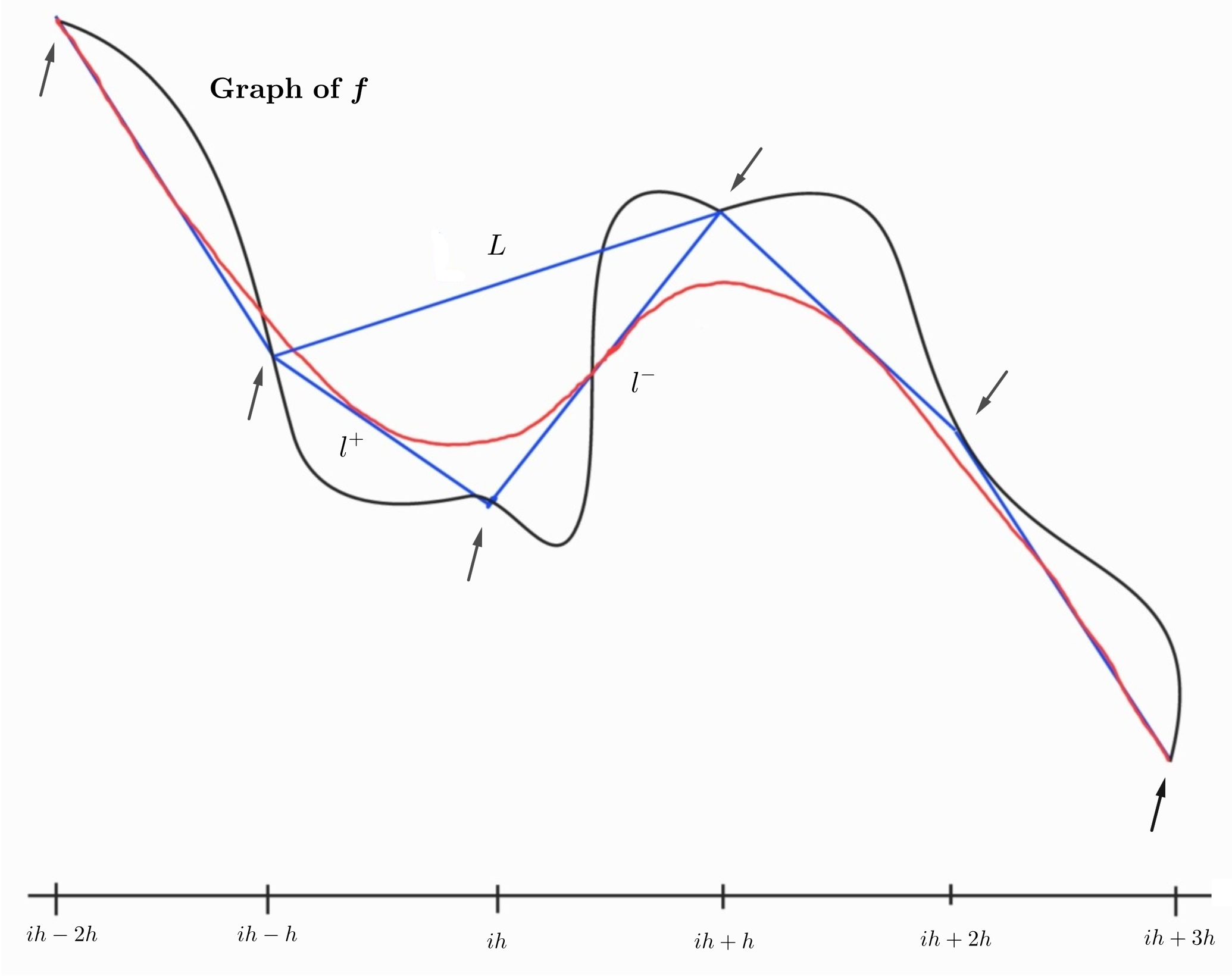
Our next aim is to show that the constant 9/8 figuring in Theorem 5.1 can be replaced by 1. To this end, it seems to be instructive to sketch the graph of a typical spline $S_{2}f$ in order to better understand the argument following.

In Figure 1, the graph of $f$ is drawn as a bold line. At the points indicated by arrows (such as $\swarrow )$, the function $f$ is interpolated by the polygonal spline $S_1\left(f\right)$ (visible as such). The quadratic spline $S_2\left(f\right)$ is then uniquely determined by the interpolation conditions (5) tot 5.1 este si in original???? and the condition of $C^1$-continuity, i.e., that the slope of $S_2\left(f\right)$ in the points $ih+\frac{h}{2},i=0,\mathrm{\dots },m-1$, equals the one of $S_1\left(f\right)$. (Thus, $S_2\left(f\right)$ can be composed of Bernstein parabolas by the well-known control point construction). Next we show

Theorem 5.3.

$\left|f\left(x\right)-S_2(f;x)\right|$ $\le {\omega }_2(f;h/2),0\le x\le h/2,\text{ or }1-h/2\le x\le 1,\text{ and}$

$\left|f\left(x\right)-S_2(f;x)\right|$ $\le {\omega }_2(f;h),h\le x\le 1-h/2.$

Figure 2. Figure 2

Figure 3. Figure 3

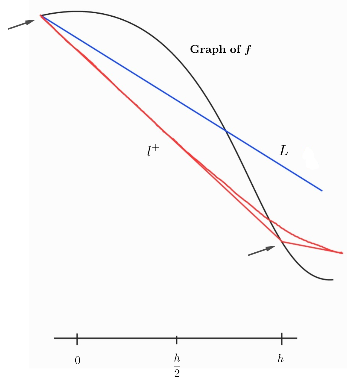
Case I: $x\in [0,\frac{h}{2}]$. Here $S_2(f;x)$ is the linear function interpolating at $f\left(0\right)$ and $f\left(h\right)$, and its graph there coincides with that of ${\mathrm{\ell }}^{+}$ below.

Since ${\mathrm{\ell }}^{+}$interpolates $f$ at $o$ and $h$, we know from Lemma 2.3 (i) that

$$\left|f\left(x\right)-S_{2}f\left(x\right)\right|=\left|f\left(x\right)-{\mathrm{\ell }}^{+}\left(x\right)\right|\le {\omega }_2{(f;x/2)}_{[0,h]}\text{ for all }x\in [0,h/2].$$

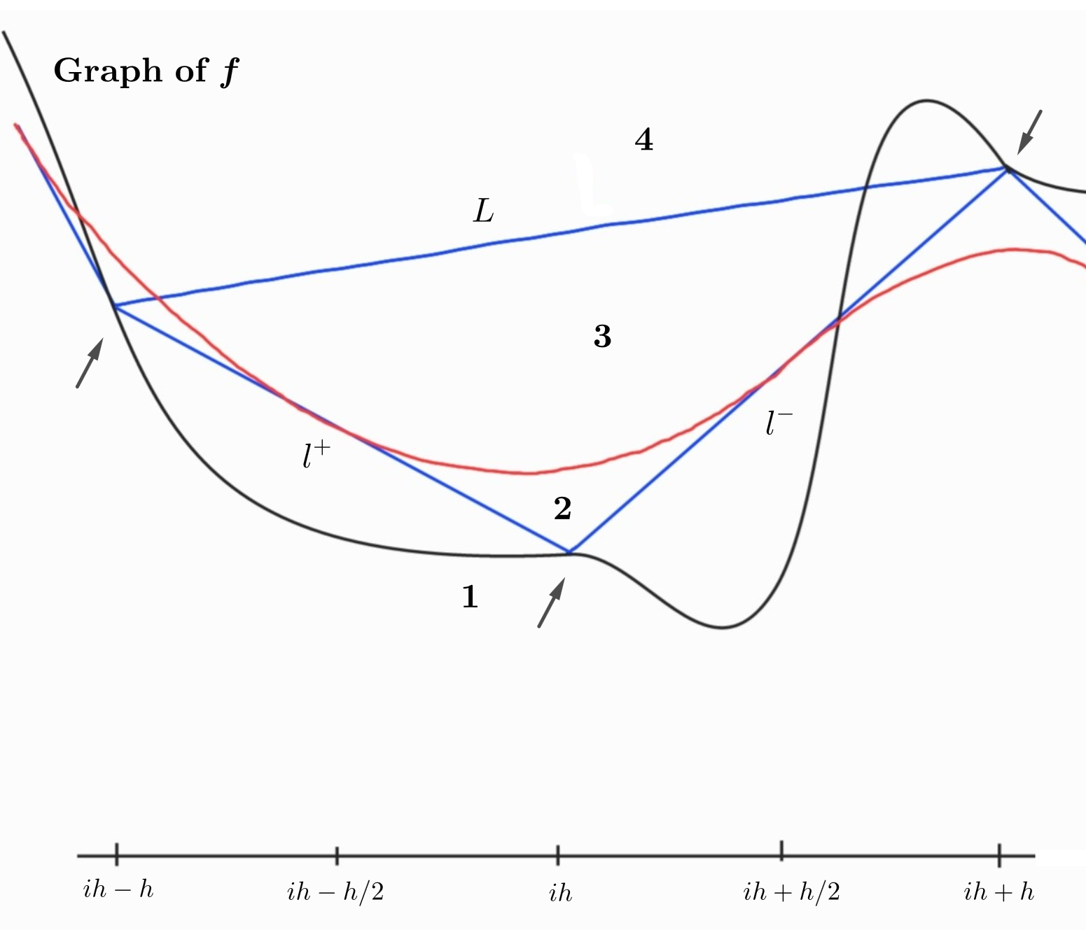
Case II: $x\in [ih-\frac{h}{2}.ih+\frac{h}{2}],i\le i\le m-1,i$ fixed. We are thus considering the following part of Figure 1.

We first look at the larger interval $[ih-h,ih+h]$ and estimate the difference $L-f$  there. Since $L$ interpolates at $ih-h$ and $ih+h$, it follows from Lemma 2.3 (i) that

$$|f\left(x\right)-L\left(x\right)|\le {\omega }_2{(f;h)}_{[ih-h,ih+h]}\text{ for all }x\in [ih-h,ih+h.]$$

The same argument shows that

$\left|f\left(x\right)-{\mathrm{\ell }}^{+}\left(x\right)\right|$ $\ge {\omega }_2{(f;h/2)}_{[ih-h,ih]}\text{ for all }x\in [ih-h,ih]\text{, and}$

$\left|f\left(x\right)-{\mathrm{\ell }}^{-}\right|$ $\le {\omega }_2{(f;h/2)}_{[ih,ih+h]}\text{ for all }x\in [ih,ih+h].$

Now observe that, by construction, over the interval $[ih-\frac{h}{2},ih+\frac{h}{2}]$ the graph of $S_{2}f$ lies inside the triangle ${△}_i$ formed by the graphs of $L,{\mathrm{\ell }}^{+}$, and ${\mathrm{\ell }}^{-}$. Furthermore, relative to the triangle ${△}_i$, the graph of $f$ can be in one of the positions indicated by 1, 2, 3, and 4 in the above figure. Therefore, for $x\in [ih-\frac{h}{2},ih]$, we have:

in cases 1 and 2: $\left|\left(f-S_{2}f\right)\left(x\right)\right|\le \left|\left(f-L\right)\left(x\right)\right|$, and

in cases 3 and 4: $\left|\left(f-S_{2}f\right)\left(x\right)\right|\le \left|\left(f-{\mathrm{\ell }}^{+}\right)\left(x\right)\right|$.

Analogous inequalities hold on $[ih,ih+\frac{h}{2}]$ with ${\mathrm{\ell }}^{+}$ replaced by ${\mathrm{\ell }}^{-}$, and hence it follows that we have

$\left|\left(f-S_{2}f\right)\left(x\right)\right|$ $\le \max \{\left|\left(f-L\right)\left(x\right)\right|,\left|\left(f-{\mathrm{\ell }}^{+}\right)\left(x\right)\right|,\left|f-{\mathrm{\ell }}^{-}\left(x\right)\right|\}$

$\le {\omega }_2{(f;h)}_{[ih-h,ih+h]}\text{ for all }x\in [ih-\frac{h}{2},ih+\frac{h}{2}].$

Case III: $x\in [1-\frac{h}{2},1]$. Here the argument is analogous to that of case 1, and hence the proof of the theorem is complete.

The statement of the next lemma parallels that of Lemma 2.4 It shows that lower order derivatives of $S_{2}f$ also behave well (note again that we are treating the case $h=\frac{1}{m}$ only).

Lemma 5.4.

Let $m\ge 2$ and $S_{2}f$ be given as above $\left(\text{i.e., }h=\frac{1}{m}\right)$. Then one has for all $f\in C[0,1]$, all $x\in [0,1]$,

$$\left|{\left(S_{2}f\right)}^{\prime }\left(x\right)\right|\le \frac{1}{h}\cdot {\omega }_1(f;h),\text{ and }\left|\left(S_{2}f\right)\left(x\right)\right|\le {\Vert f\Vert }_{\mathrm{\infty }}.$$

Proof.

Case I: $x\in [0,\frac{h}{2}]$. Here $S_2(f;x)$ is the linear function interpolating at $f\left(h\right)$ and $f\left(0\right)$, and thus

$$\left|{\left(S_{2}f\right)}^{\prime }\left(x\right)\right|=\frac{1}{h}\cdot \left|f\left(h\right)-f\left(0\right)\right|\le \frac{1}{h}\cdot {\omega }_1(f;h).$$

Case II: $x\in [ih-\frac{h}{2},ih+\frac{h}{2}],1\le i\le m-1$. In these intervals $S_{2}f$ is the second degree Bernstein polynomial determined by the ordinates $S_1(f;ih-\frac{h}{2}),S_{1}f\left(ih\right)=f\left(ih\right)$, and $S_1(f;ih+\frac{h}{2})$. Differentiating this polynomial once gives

$\frac{2}{h^2}\cdot {\displaystyle \sum _{j=0}^1}{△}_{\frac{h}{2}}^1\left(S_{1}f\right)\left(ih-\frac{h}{2}+j\cdot \frac{h}{2}\right)\cdot \left(\genfrac{}{}{0pt}{}{1}{j}\right)\cdot {\left[x-\left(ih-\frac{h}{2}\right)\right]}^j{\left(ih+\frac{h}{2}-x\right)}^{1-j}\le$

$\le \frac{2}{h^2}h\max \{\left|S_{1}f\left(ih-\frac{h}{2}\right)-S_{1}f\left(ih\right)\right|,\left|S_{1f}\left(ih\right)-S_{1f}\left(ih+\frac{h}{2}\right)\right|\}$

$=\frac{1}{h}\cdot \max \{\left|f\left(ih-h\right)-f\left(ih\right)\right|,\left|f\left(ih\right)-f\left(ih+h\right)\right|\}$

$\le \frac{1}{h}\cdot {\omega }_1(f;h).$

The case $x\in [1-\frac{h}{2},1]$ can be treated analogously to that of $x\in [0,\frac{h}{2}]$.

In order to see that ${\Vert S_{2}f\Vert }_{\mathrm{\infty }}\le {\Vert f\Vert }_{\mathrm{\infty }}$, it is only necessary to observe that the convex hull of the graph of $f$ encloses that of S${}_1{}^{}f$, and that the convex hull of the graph of $S_{1}f$ encloses the one of $S_{2}f$.

∎

As we mentioned in Remark 5.2 , we were unable to verify Sendov’s Theorem 5.1 for all . It is thus natural to state

Problem 5.5.

Let $f\in C[0,1]$ and be given. Is it true there are functions $f_h\in W_{2,\mathrm{\infty }}[0,1]$ such that the following hold:

• ${\Vert f-f_h\Vert }_{\mathrm{\infty }}\le {\omega }_2(f;h),$

• ${\Vert f_h^{\prime \prime }\Vert }_{L_{\mathrm{\infty }}}\le h^{-2}\cdot {\omega }_2(f;h),$

• ${\Vert f_h^{\prime }\Vert }_{\mathrm{\infty }}\le h^{-1}\cdot {\omega }_1(f;h),$

• ${\Vert f_h\Vert }_{\mathrm{\infty }}\le {\Vert f\Vert }_{\mathrm{\infty }}$

Acknowledgements.

The authors gratefully acknowledge Claudia Cottin, Rita Hülsbusch, Eva Müller-Faust, John Sevy, Hans-Jörg Wenz  and Xin-long Zhou for their technical help in preparing this note, for their critical remarks on earlier versions, or for several attempts to solve 5.5.

References

- [1] J.A. Adell, J. de la Cal, Preservation of moduli of continuity for Bernstein-type operators, Manuscript 1993. https://doi.org/10.1007/978-1-4615-2494-6_1
- [2] G.A. Anastassiou, C. Cottin, H.H., Gonska, Global smoothness of approximating functions, Analysis, 11 (1991), pp. 43–57. https://doi.org/10.1524/anly.1991.11.1.43
- [3] I.B. Bashmakova, On approximation by Hermite splines (Russian), In: Numerical Methods in Boundary Value Problems of Mathematical Physics (Meshvyz. Temat. Sb. Tr.), 5-7. Leningrad: Leningradskii Inzhemerno-Stroitel’nyi Institut,1985.
- [4] W.R. Bloom, D. Elliot, The modulus of continuity of the remainder in the approximation of Lipschitz functions, J. Approx. Theory, 31 (1981), pp. 59–66. https://doi.org/10.1016/0021-9045(81)90030-7
- [5] C. Badea, I. Badea, H. Gonska, Improved estimates on simultaneous approximation by Bernstein operators II, Manuscript 1993.
- [6] A. Boos, Jia-ding Cao, H. Gonska, Approximation by Boolean sums of positive linear operators V: on the constants in DeVore-Gopengauz-type inequalities. To appear in Calcolo. Temporary reference: Schriftenreihe des Instituts für Angewandte Informatik SIAI-EBS-4-93, European Business School, 1993. https://doi.org/10.1007/BF02575858
- [7] Ju.A.Brudnyi, Approximation of functions of variables by quasi-polynomials (Russian), Izv. Akad. Nauk SSSR, Ser. Mat., 34 (1970), pp. 564–583. English translation: Math. USSR-Izvestija 4 (1970, n.3), pp. 568–586. https://doi.org/10.1070/IM1970v004n03ABEH000922
- [8] H. Burkill, Cesàro-Perron almost periodic functions, Proc. London Math. Soc (Series 3), 2 (1952), pp. 150–174. https://doi.org/10.1112/plms/s3-2.1.150
- [9] Jia-ding Cao, H. Gonska, Approximation by Boolean sums of positive linear operators, Rend. Mat. 6 (1986), 525-546.
- [10] C. Cottin, H. Gonska, Simultaneous approximation and global smoothness preservation, Rend. Circ. Mat. Palermo (2) Suppl. 33 (1993), pp. 259–279.
- [11] R.A. Devore, The Approximation of Continuous Functions by Positive Linear Operators, Berlin: Springer 1972. https://doi.org/10.1007/BFb0059493
- [12] R.A. Devore, Degree of approximation, in ?? ?? Approximation Theory II?? ?? . (Proc. Int. Symp. Austin 1976; ed. by G.G. Lorentz et al.), pp. 117–161. New York: Academic Press 1976.
- [13] G. Freud, Su i procedimenti lineari d’approssimazione, Atti Accad. Naz. Lincei, Rend. Cl. Sci. Fis. Mat. Natur. 26 (1959), pp. 641–643.
- [14] N.G. Gasharov, On estimates for the approximation by linear operators preserving linear functions (Russian), In: ”Approximation of Functions by Special Classes of Operators”. 28035, Vologda, 1987.
- [15] N.G. Gasharov, Written comunication, January 1992.
- [16] I. Gavrea, About a conjecture, Studia Univ. Babeş-Bolyai Math. 38 (1993).
- [17] I. Gavrea, I. Raşa, Remarks on some quantitative Korovkin-type results, Manuscript 1993.
- [18] H.H. Gonska, Query in ?? ?? Unsolved Problems?? ?? ,In: ?? ?? Constructive Function Theory’81?? ?? .(Proc.Int.Conf.Varna 1981; ed. by Bl. Sendov et. al.), pp. 597–598, Sofia: Publishing House of the Bulgarian Acadmy of Sciences 1983.
- [19] H.H. Gonska, Two problems on best constants in direct estimates, In: Problem Section of Proc. Section Edmonton Conf. Approximation Theory (Edmonton, Alta., 1982; ed. by Z. Ditzian et al., 194, Providence, RI: Amer. Math. Soc. 1983.
- [20] H.H. Gonska, Quantitative Korovkin-type theorems on simultaneous approximation, Math. Z., 186 (1984), pp. 419–433. https://doi.org/10.1007/BF01174895
- [21] H.H. Gonska, Degree of approximation by lacunary interpolators: interpolation, Rocky Mountain J. Math. 19 (1989), pp. 157–171. https://doi.org/10.1216/RMJ-1989-19-1-157
- [22] H.H. Gonska, J. Meier, On approximation by Bernstein type operators: best constants, Studia Sci. Math. Hungar., 22 (1987), pp. 287–297.
- [23] H.H. Gonska, Ding-xuan Zhou, On an extremal problem concerning Bernstein operators, To appear in Serdica. Temporary reference: Schriftenreihe des Instituts für Angewandte Informatik SIAI-EBS-10-94, European Business School 1994.
- [24] H.H. Gonska, Xin-long Zhou, Polynomial approximation with side conditions: recent results and open problems, In:?? ?? Proc. First International Colloquium on Numerical Analysis (Plovdiv 1992; ed. by D.Bainov and V. Covachev), 61-71. Zeist/The Netherlands: VPS International Science Publishers 1993. https://doi.org/10.1515/9783112314111-007
- [25] D.S. Mitrinovic, Analytic Inequalities, Berlin et al: Springer 1970. https://doi.org/10.1007/978-3-642-99970-3
- [26] R. Păltănea, On the estimate of the pointwise approximation of functions by linear positive functionals, Studia Univ. Babes-Bolyai 53 (1990), no.1, pp. 11–24.
- [27] L.L. Schumaker, Spline Functions: Basic Theory, New York: John Wiley & Sons 1981.
- [28] Bl. Sendov, On a theorem of Ju. Brudnyi, Math. Balkanica (N.S.), 1 (1987), no.1, pp. 106–111.
- [29] Bl. Sendov, V.A. Popov, Averaged Moduli of Smoothness (Bulgarian), Sofia: Publishing House of the Bulgarian Academy of Sciences 1983.
- [30] Bl. Sendov, V.A. Popov, The Averaged Moduli of Smoothness, New York: John Wiley & Sons 1988.
- [31] P.C. Sikkema, Der Wert einiger Konstanten in der Theorie der Approximation mit Bernstein-Polynomen, Numer. Math.,3 (1961), pp. 107–116. https://doi.org/10.1007/BF01386008
- [32] S.B. Stečkin, The approximation of periodic functions by Féjer sums (Russian), Trudy Mat. Inst. Steklov 62 (1961), 48-60, English translation: Amer. Math. Soc. Transl., (2) 28 (1963), pp. 269–282. https://doi.org/10.1090/trans2/028/14
- [33] H. Withney, On functions with bounded -th differences, J. Math. Pures et Appl., 36 (1957), pp. 67–95.
- [34] Ding-xuan Zhou, On a problem of Gonska. To appear in Resultate Math.
- [35] V.V. Zhuk, Functions of the Lip 1 class and S.N. Bernstein’s polynomials (Russian), Vestnik Leningrad.Univ. Math Mekh. Astronom. 1989, vyp.1, pp. 25–30.