A new preconditioned Richardson iterative method

Abstract.

This paper proposes a new iterative technique for solving a linear system $Ax=y$ based on the Richardson iterative method. Then using the Chebyshev polynomials, we modify the proposed method to accelerate the convergence rate. Also, we present the results of some numerical experiments that demonstrate the efficiency and effectiveness of the proposed methods compared to the existing, state-of-the-art methods.

1. Introduction and preliminaries

Linear systems arise in various scientific and engineering applications, including differential equations, signal processing, and optimization [4, 5, 6, 7, 8, 12]. Therefore, it is crucial to find the efficient solution of a linear system in both theoretical and practical contexts. Iterative methods of solving linear systems have been extensively studied because they are more efficient than direct methods when solving large-scale problems. Furthermore, iterative methods have the advantage of being easily adaptable to different types of linear operators, which makes them versatile and applicable to a broad range of problems. Such operators frequently arise in practical applications, including image processing and machine learning.

In the present work, we propose a new iterative method for solving linear systems with bounded, self-adjoint operators and then present a new, modified version of the process by using the Chebyshev polynomials. The method utilizes a flexible preconditioner that adapts to the structure of the operator and exploits its self-adjointness. The resulting algorithms have favorable convergence properties and require fewer iterations than some existing methods. Also, we present the results of some numerical experiments that demonstrate the efficiency and effectiveness of our methods compared to the existing, state-of-the-art methods.

Consider the linear system

(1) $$Ax=y$$

in a Hilbert space $\mathscr{H}$, where $A$ is a bounded and self-adjoint operator. The basic idea of an iterative method is to use an initial guess $x_0$, and then apply a sequence of updates to the solution, refining the solution with each iteration. There are many different iterative methods, each having its advantages and disadvantages, depending on the properties of the equation to be solved.

The most straightforward approach to an iterative solution is to rewrite (1) as a linear, fixed point iteration. If we consider the function $ℒ(x)=Ax+x-y$ on $\mathscr{H}$, then $x^{\ast }$ is a solution of $Ax=y$ if and only if $x^{\ast }$ is a fixed point of $ℒ$. Thus, it seems natural to consider fixed-point theorems.

One of the best and most widely used methods to do this is the Richardson iterative method [12]. The abstract Richardson iterative method has the form

(2) $$x_k=x_{k-1}+\alpha r_{k-1},$$

where and $r_k$ is the residual vector $y-A{x}_k$. Note that we can rewrite (2) as

$$x_k=(I-\alpha A)x_{k-1}+\alpha y.$$

The Conjugate Gradient method is a more sophisticated method that uses information about the residual error to guide the iterative updates [12]. The update for the $k$th iteration is given by

$$x_k=x_{k-1}+{\alpha }_k{p}_k,$$

where ${\alpha }_k$ is the step size, $p_k$ is the search direction given by

$$p_k=r_{k-1}+{\beta }_k{p}_{k-1},$$

and

$$r_k=y-A{x}_k$$

is the residual, with ${\beta }_k$ determined by the Conjugate Gradient method.

However, it is possible to precondition the linear equation (1) by multiplying both sides by an operator $B$ to obtain $BAx=By$, so that the convergence of the iterative methods is improved. In this case, the residual $By-BA{x}_k$ better reflects the actual error. This method is a very effective technique for solving differential equations, integral equations, and related problems [2, 9, 10].

In general, iterative methods are powerful tools for solving large systems of linear equations. By choosing an appropriate iterative method based on the properties of the operator under consideration, it is possible to obtain fast and accurate solutions to a wide range of linear systems.

2. Preconditioning the problem based on Richardson’s method

Based on the properties of the operator $A$ in equation (1), positive constants $c_1$ and $c_2$ exist such that for each $u\in \mathscr{H}$,

(3) $$\sqrt{c_1}{\Vert u\Vert }_{\mathscr{H}}\le {\Vert Au\Vert }_{\mathscr{H}}\le \sqrt{c_2}{\Vert u\Vert }_{\mathscr{H}}.$$

Although the positive definiteness of $A$ is essential for methods such as conjugate gradient, our method can disregard this property. This is more evident in the Numerical results section.

It is not difficult to show that the optimal parameters $c_1$ and $c_2$ in equation (3) are equal to ${\lambda }_{\min }(A^2)$ and ${\lambda }_{\max }(A^2)$, respectively. Considering the properties of matrix $A$, there exist constants $c_1$ and $c_2$ that satisfy the aforementioned equation. It is not imperative to utilize the optimized coefficients within this context. Consequently, precise knowledge of the eigenvalues of the matrix $A^2$ is not mandatory; an approximation thereof is sufficient.
Now, based on the Richardson iterative method, we consider the iteration

(4) $$x_k=x_{k-1}+\frac{4}{c_1+c_2}\left(I-\frac{1}{c_1+c_2}{A}^2\right)A\left(y-A{x}_{k-1}\right).$$

In this case, the following lemma holds.

Lemma 1.

Let $A$ be a bounded and self-adjoint operator on a Hilbert space $\mathscr{H}$. Then

$$\Vert I-\frac{4}{c_1+c_2}\left(I-\frac{1}{c_1+c_2}{A}^2\right)A^2\Vert \le {\left(\frac{c_2-c_1}{c_2+c_1}\right)}^2,$$

where $c_1$ and $c_2$ are the constants used in (3).

Proof.

Since $A$ is self-adjoint, for each $x\in \mathscr{H}$ we obtain

$⟨\left(I-\frac{2}{c_1+c_2}{A}^2\right)x,x⟩$ $={\Vert x\Vert }_{\mathscr{H}}^2-\frac{2}{c_1+c_2}⟨A^{2}x,x⟩$

$={\Vert x\Vert }_{\mathscr{H}}^2-\frac{2}{c_1+c_2}⟨Ax,Ax⟩={\Vert x\Vert }_{\mathscr{H}}^2-\frac{2}{c_1+c_2}{\Vert Ax\Vert }_{\mathscr{H}}^2$

$\le {\Vert x\Vert }_{\mathscr{H}}^2-\frac{2c_1}{c_1+c_2}{\Vert x\Vert }_{\mathscr{H}}^2=\left(\frac{c_2-c_1}{c_2+c_1}\right){\Vert x\Vert }_{\mathscr{H}}^2,$

where the inequality follows from (3).

Similarly, we can prove that for every $x\in \mathscr{H}$,

$$-\left(\frac{c_2-c_1}{c_2+c_1}\right){\Vert x\Vert }_{\mathscr{H}}^2\le ⟨\left(I-\frac{2}{c_1+c_2}{A}^2\right)x,x⟩.$$

Therefore,

(5) $${\Vert I-\frac{2}{c_2+c_1}{A}^2\Vert }_{\mathscr{H}}\le \left(\frac{c_2-c_1}{c_2+c_1}\right).$$

Finally, inequality (5) allows us to conclude that

${\Vert I-\frac{4}{c_1+c_2}\left(I-\frac{1}{c_1+c_2}{A}^2\right)A^2\Vert }_{\mathscr{H}}$ $={\Vert I-\frac{4}{c_1+c_2}{A}^2+\frac{4}{{(c_1+c_2)}^2}{A}^4\Vert }_{\mathscr{H}}$

$={\Vert {\left(I-\frac{2}{c_1+c_2}{A}^2\right)}^2\Vert }_{\mathscr{H}}$

$\le {\Vert \left(I-\frac{2}{c_1+c_2}{A}^2\right)\Vert }_{\mathscr{H}}^2$

$\le {\left(\frac{c_2-c_1}{c_2+c_1}\right)}^2,$

which completes the proof. ∎

Note that the optimal convergence rate in the Richardson iterative method, obtained by letting $\alpha =\frac{2}{{\lambda }_{\min }(A)+{\lambda }_{\max }(A)}$, is $\frac{{\lambda }_{\max }(A)+{\lambda }_{\min }(A)}{{\lambda }_{\max }(A)+{\lambda }_{\min }(A)}$.
In the following theorem, we show that the convergence rate of the iterative method (4) is ${\left(\frac{c_2-c_1}{c_2+c_1}\right)}^2$.

Theorem 2.

For any initial guess $x_0$ of the solution of (1), the sequence ${\{x_k\}}_{k=0}^{\mathrm{\infty }}$ defined by (4) converges to the exact solution $x^{\ast }$ of (1) with convergence rate equal to ${\left(\frac{c_2-c_1}{c_2+c_1}\right)}^2$.

Proof.

The definition of $x_k$ in (4) leads to

$$x^{\ast }-x_k=x^{\ast }-x_{k-1}-\frac{4}{c_1+c_2}\left(I-\frac{1}{c_1+c_2}{A}^2\right)A\left(y-A{x}_{k-1}\right),$$

$x^{\ast }-x_{k-1}-\left(\frac{4}{c_1+c_2}I-\frac{4}{{(c_1+c_2)}^2}{A}^2\right)A^2\left(x^{\ast }-x_{k-1}\right)=$

$=\left(I-\frac{4}{c_1+c_2}{A}^2+\frac{4}{{(c_1+c_2)}^2}{A}^4\right)\left(x^{\ast }-x_{k-1}\right)$

$={\left(I-\frac{2}{c_1+c_2}{A}^2\right)}^2\left(x^{\ast }-x_{k-1}\right).$

Therefore,

${\Vert x^{\ast }-x_k\Vert }_{\mathscr{H}}$ $={\Vert {\left(I-\frac{2}{c_1+c_2}{A}^2\right)}^2\left(x^{\ast }-x_{k-1}\right)\Vert }_{\mathscr{H}}$

$\le {\Vert \left(I-\frac{2}{c_1+c_2}{A}^2\right)\Vert }_{\mathscr{H}}^2{\Vert \left(x^{\ast }-x_{k-1}\right)\Vert }_{\mathscr{H}}.$

Thus, the result follows from the previous lemma. ∎

Note: Assume $c_1^{\ast }={\lambda }_{\min }(A^2)$ and $c_2^{\ast }={\lambda }_{\max }(A^2)$. Let $c_1=c_1^{\ast }-\delta$ and $c_2=c_2^{\ast }+\delta$, then $c_1+c_2=c_1^{\ast }+c_2^{\ast }$ and $c_2-c_1=c_2^{\ast }-c_1^{\ast }+2\delta$. Therefore, since ${\left(\frac{c_2^{\ast }-c_1^{\ast }}{c_2^{\ast }+c_1^{\ast }}\right)}^2\le {\left(\frac{c_2-c_1}{c_2+c_1}\right)}^2$, Lemma 1 and so Theorem 2 hold in this case.

To summarize the results obtained so far, we present an algorithm that generates an approximate solution to equation (1) with prescribed accuracy.

Algorithm 1 $[A,c_1,c_2,ϵ]⟶x_{ϵ}$

1. Let $\rho ={\left(\frac{c_2-c_1}{c_2+c_1}\right)}^2$.

2. $k=0,x_k=0$.

3. $k=k+1,r_{k-1}:=y-x_{k-1},v_{k-1}:=A{r}_{k-1},w_{k-1}=A{v}_{k-1}$,

a) $x_k=x_{k-1}+\frac{4}{c_2+c_1}\left(v_{k-1}-\frac{1}{c_2+c_1}A{w}_{k-1}\right)$,

b) ${\rho }_k={\rho }^k\frac{1}{\sqrt{c_1}}{\Vert y\Vert }_{\mathscr{H}}$.

4. If , then stop and set $u_{ϵ}=x_k$ as an approximate solution. Otherwise, go to Step (3).

3. Modification by Chebyshev polynomials

In this section, the properties of the Chebyshev polynomials are used to modify the previous algorithm to accelerate the convergence rate.

Considering the iteration (3), let $u_n={\sum }_{k=1}^n{a}_{n_k}{x}_k$, where ${\sum }_{kj=1}^n{a}_{n_k}=1$. In this case, based on the proof of the previous theorem,

$x^{\ast }-u_n$ $={\displaystyle \sum _{k=1}^n}{a}_{n_k}{x}^{\ast }-{\displaystyle \sum _{k=1}^n}{a}_{n_k}{x}_k={\displaystyle \sum _{k=1}^n}{a}_{n_k}(x^{\ast }-x_k)=$

$={\displaystyle \sum _{k=1}^n}{a}_{n_k}{\left(I-\frac{2}{c_1+c_2}{A}^2\right)}^{2k}\left(x^{\ast }-x_0\right).$

By setting $B={\left(I-\frac{2}{c_1+c_2}{A}^2\right)}^2$ and $P_n(x)={\sum }_{k=1}^n{a}_{n_k}{x}^k$, we see that

(6) $$x^{\ast }-u_n=\sum _{k=1}^n{a}_{n_k}{B}^k\left(x^{\ast }-x_0\right)=P_n(B)\left(x^{\ast }-x_0\right).$$

Since $A$ is invertible and self-adjoint, $A^2$ is a positive definite operator. Also, by the previous lemma, the spectrum of $B$ is a subset of the interval $[-\rho ,\rho ]$, where $\rho ={\left(\frac{c_2-c_1}{c_2+c_1}\right)}^2$. Therefore, in view of (6), the spectral theorem leads to

(7) ${\Vert x^{\ast }-u_n\Vert }_{\mathscr{H}}$ $={\Vert P_n(B)\left(x^{\ast }-x_0\right)\Vert }_{\mathscr{H}}\le \Vert P_n(B)\Vert {\Vert x^{\ast }-x_0\Vert }_{\mathscr{H}}$

$\le \underset{|x|\le \rho }{\max }|P_n(x)|{\Vert x^{\ast }-x_0\Vert }_{\mathscr{H}}.$

In the sequel, we aim to minimize ${\Vert x^{\ast }-u_n\Vert }_{\mathscr{H}}$. We have to find

(8) $$\underset{P_n\in {\mathbb{P}}_n}{\min }\underset{|x|\le \rho }{\max }|P_n(x)|,$$

where ${\mathbb{P}}_n:=\{P_n(x):P_n(x)$ is a polynomial of degree $n$ with $P_n(1)=1.\}$.

We investigate the solution to this problem in terms of the Chebyshev polynomials [3]. These polynomials are defined by

and satisfy the recurrence relations

$$c_0(x)=1,c_1(x)=x,c_n(x)=2x{c}_{n-1}(x)-c_{n-2}(x),\forall n\ge 2.$$

The following lemma presents a minimization property of these polynomials which will be used later.

Lemma 3 ([3]).

Let and set

$$Q_n(x)=\frac{c_n\left(\frac{2x-a-b}{b-a}\right)}{c_n\left(\frac{2-a-b}{b-a}\right)}$$

for $x\in [a,b]$. Then, for each $P_n\in {\mathbb{P}}_n$,

$$\underset{a\le x\le b}{\max }|Q_n(x)|\le \underset{a\le x\le b}{\max }|P_n(x)|.$$

Furthermore,

$$\underset{a\le x\le b}{\max }|Q_n(x)|=\frac{1}{c_n\left(\frac{2-a-b}{b-a}\right)}.$$

This lemma shows that the minimization problem (8) can be solved by setting $a=-\rho$ and $b=\rho$. These lead to

(9) $$Q_n(x)=\frac{c_n\left(\frac{x}{\rho }\right)}{c_n\left(\frac{1}{\rho }\right)},$$

which solves (8).

Now, we rewrite $u_k$ by using the Chebyshev polynomials. First of all, combining (9) with the definition of the Chebyshev polynomials (the recurrence relation) for $n\ge 2$, we obtain

$c_n(\frac{1}{\rho })Q_n(x)$ $=c_n(\frac{x}{\rho })=\frac{2x}{\rho }{c}_{n-1}({\displaystyle \frac{x}{\rho }})-c_{n-2}(\frac{x}{\rho })$

$=\frac{2x}{\rho }{c}_{n-1}(\frac{1}{\rho })Q_{n-1}(x)-c_{n-2}(\frac{1}{\rho })Q_{n-2}(x).$

Replacing $x$ with $B$ and applying the resulting operator identity to $x^{\ast }-x_0$ yield

$$c_n(\frac{1}{\rho })Q_n(B)=\frac{2B}{\rho }{c}_{n-1}(\frac{1}{\rho })Q_{n-1}(B)(x^{\ast }-x_0)-c_{n-2}(\frac{1}{\rho })Q_{n-2}(B)(x^{\ast }-x_0).$$

By (6) and the fact that $Q_n(x)$ is the solution of the minimization problem (8), the above equation can be recovered as

$$c_n(\frac{1}{\rho })(x^{\ast }-u_n)=\frac{2}{\rho }{c}_{n-1}(\frac{1}{\rho })B(x^{\ast }-u_{n-1})-c_{n-2}(\frac{1}{\rho })(x^{\ast }-u_{n-2}),$$

or equivalently,

$c_n(\frac{1}{\rho })(x^{\ast })-c_n(\frac{1}{\rho })(u_n)=$

$=\frac{2}{\rho }{c}_{n-1}(\frac{1}{\rho }){\left(I-\frac{2}{c_1+c_2}{A}^2\right)}^2(x^{\ast }-u_{n-1})-c_{n-2}(\frac{1}{\rho })(x^{\ast }-u_{n-2})$

$=\frac{2}{\rho }{c}_{n-1}(\frac{1}{\rho })x^{\ast }+\frac{2}{\rho }{c}_{n-1}(\frac{1}{\rho })\left[-u_{n-1}-\left(\frac{4}{c_1+c_2}{A}^2-\frac{4}{{(c_1+c_2)}^2}{A}^4\right)(x^{\ast }-u_{n-1})\right]$

$-c_{n-2}(\frac{1}{\rho })(x^{\ast })+c_{n-2}(\frac{1}{\rho })(u_{n-2}).$

Repeated application of the recurrence relations of the Chebyshev polynomials for $n\ge 2$ leads to

$c_n(\frac{1}{\rho })u_n$ $=\frac{2}{\rho }{c}_{n-1}(\frac{1}{\rho })\left[u_{n-1}+\left(\frac{4}{c_1+c_2}{A}^2-\frac{4}{{(c_1+c_2)}^2}{A}^4\right)(x^{\ast }-u_{n-1})\right]$

$-c_{n-2}(\frac{1}{\rho })(u_{n-2}),$

and hence

(10) $u_n$ $=\frac{2}{\rho }\frac{c_{n-1}(\frac{1}{\rho })}{c_n(\frac{1}{\rho })}\left[u_{n-1}+\left(\frac{4}{c_1+c_2}{A}^2-\frac{4}{{(c_1+c_2)}^2}{A}^4\right)(x^{\ast }-u_{n-1})\right]$

$-\frac{c_{n-2}(\frac{1}{\rho })}{c_n(\frac{1}{\rho })}(u_{n-2}).$

If we set

$${\rho }_n=\frac{2}{\rho }\frac{c_{n-1}(\frac{1}{\rho })}{c_n(\frac{1}{\rho })},$$

then according to the properties of the Chebyshev polynomials we obtain

$$1-{\rho }_n=-\frac{c_{n-2}(\frac{1}{\rho })}{c_n(\frac{1}{\rho })}.$$

Therefore, we can rewrite (10) as

$$u_n={\rho }_n\left[u_{n-1}+\left(\frac{4}{c_1+c_2}{A}^2-\frac{4}{{(c_1+c_2)}^2}{A}^4\right)(x^{\ast }-u_{n-1})\right]+(1-{\rho }_n)u_{n-2},$$

or equivalently,

$$u_n={\rho }_n\left[u_{n-1}-u_{n-2}+\left(\frac{4}{c_1+c_2}{A}^2-\frac{4}{{(c_1+c_2)}^2}{A}^4\right)(x^{\ast }-u_{n-1})\right]+u_{n-2}.$$

This yields

(11) $$u_n={\rho }_n\left[u_{n-1}-u_{n-2}+\frac{4}{c_1+c_2}\left(I-\frac{1}{(c_1+c_2)}{A}^2\right)A\left(y-A{u}_{n-1}\right)\right]+u_{n-2}.$$

Also, a straightforward computation gives us the following recursive relation for ${\rho }_n$,

(12) $${\rho }_n={\left(1-\frac{{\rho }^2}{4}{\rho }_{n-1}\right)}^{-1}.$$

Now, based on the recursive relation (12), we design the following algorithm to approximately solve equation (1).

Algorithm 2 [$A$,$c_1$,$c_2$,$ϵ$]$⟶u_{ϵ}$

1. Let $\rho ={\left(\frac{c_2-c_1}{c_2+c_1}\right)}^2$, $\sigma =\frac{\sqrt{c_1^2+c_2^2}-\sqrt{2c_1{c}_2}}{\sqrt{c_1^2+c_2^2}+\sqrt{2c_1{c}_2}}$.

2. Set $u_0=0$, $u_1=\frac{4}{c_2+c_1}\left(I-\frac{1}{c_2+c_1}{A}^2\right)Ay$, ${\rho }_1=2$, $n=1$.

3. While $\frac{2{\sigma }^n}{1+{\sigma }^{2n}}\frac{{\Vert y\Vert }_{\mathscr{H}}}{\sqrt{c_1}}>ϵ$ Do,

i) $n=n+1$;

ii) ${\rho }_n={\left(1-\frac{{\rho }^2}{4}{\rho }_{n-1}\right)}^{-1}$;

iii) $u_n={\rho }_n\left[u_{n-1}-u_{n-2}+\frac{4}{c_1+c_2}\left(I-\frac{1}{\left(c_1+c_2\right)}{A}^2\right)A\left(y-A{u}_{n-1}\right)\right]+u_{n-2}$.

4. $u_{ϵ}=u_n$.

The following theorem investigates the convergence rate of the Algorithm.

Theorem 4.

If $x^{\ast }$ is the exact solution of (1), then the approximate solution $u_n$ given in Algorithm 2 satisfies

$${\Vert x^{\ast }-u_n\Vert }_{\mathscr{H}}\le \frac{2{\sigma }^n}{1+{\sigma }^{2n}}\frac{{\Vert y\Vert }_{\mathscr{H}}}{\sqrt{c_1}}.$$

Also, the output $u_{ϵ}$ of Algorithm 2 satisfies

Proof.

Letting $x_0$, $u_0=0$, Lemma 3 and relation (7) allow us to write

(13) $${\Vert x^{\ast }-u_n\Vert }_{\mathscr{H}}\le \frac{1}{c_n(\frac{1}{\rho })}{\Vert x^{\ast }-u_0\Vert }_{\mathscr{H}}=\frac{1}{c_n(\frac{1}{\rho })}{\Vert x^{\ast }\Vert }_{\mathscr{H}}\le \frac{1}{c_n(\frac{1}{\rho })}\frac{{\Vert y\Vert }_{\mathscr{H}}}{\sqrt{c_1}}.$$

By definition of Chebyshev polynomials and with a few straightforward calculations, we obtain

$c_n(\frac{1}{\rho })$ $=c_n{\left(\frac{c_2+c_1}{c_2-c_1}\right)}^2$

$=\frac{1}{2}\left[{\left(\frac{\left(\sqrt{c_1^2+c_2^2}+\sqrt{2c_1{c}_2}\right)}{\left(\sqrt{c_1^2+c_2^2}-\sqrt{2c_1{c}_2}\right)}\right)}^n+{\left(\frac{\left(\sqrt{c_1^2+c_2^2}+\sqrt{2c_1{c}_2}\right)}{\left(\sqrt{c_1^2+c_2^2}-\sqrt{2c_1{c}_2}\right)}\right)}^{-n}\right].$

Thus, by setting

$$\sigma =\frac{\sqrt{c_1^2+c_2^2}-\sqrt{2c_1{c}_2}}{\sqrt{c_1^2+c_2^2}+\sqrt{2c_1{c}_2}}$$

we conclude that

$$c_n(\frac{1}{\rho })=\frac{1}{2}\left(\frac{1}{{\sigma }^n}+{\sigma }^n\right)=\frac{1+{\sigma }^{2n}}{2{\sigma }^n}.$$

Combining this equality with a relation (13), we obtain the desired result. ∎

It is expected that methods utilizing more spectral information to yield better results compared to those relying solely on matrix-vector products. However, the exact eigenvalues are not necessary for our method, as we assume that the coefficients $c_1$ and $c_2$ exist.

4. Numerical results

In this section, we present several examples to evaluate the efficiency and performance of our algorithms and compare them with several well-known algorithms in some cases. In addition, we compare our algorithms, namely, Algorithm 1 and Algorithm 2, with each other as well as with the Richardson and Conjugate Gradient (CG) algorithms in some cases.

The reported experiments were performed on a 64-bit 2.4 GHz system using MATLAB version 2010.

In the following two examples, we show the efficiency of our novel algorithms by using $3\times 3$ and $5\times 5$ systems, respectively. Both examples use the tolerance threshold $ϵ=0.001$.

Example 5.

Let

Since

it is straightforward to investigate that $A$ is invertible, self-adjoint and positive definite. Assuming

$$f=\left[\begin{array}{c}1\\ 4\\ -6\end{array}\right]$$

and concluding $c_1={\lambda }_{\min }(A^2)=81$ and $c_2={\lambda }_{\max }(A^2)=1511700$, the following results are obtained for the system $Ax=f$ .

The exact solution for this system is

$$x^{\ast }=\left[\begin{array}{c}0.2376\\ 0.1336\\ -0.0397\end{array}\right]$$

and as mentioned above, the given tolerance threshold is $ϵ=0.001$. First, we use Algorithm 1 to approximate the solution of this system. By using Algorithm 1, we obtain the approximate solution $g_k$ after $31232$ iterations within $t=0.167103$ $sec.$ Also, Algorithm 2 gives an approximation of the solution within $t=0.0073$ $sec.$ after only $353$ iterations.

As discussed in Section 2, it is unnecessary to utilize the optimal values of $c_1$ and $c_2$ as the eigenvalues of the matrix $A^2$; a mere approximation is sufficient. Methods such as the Power Method [13] and the Jacobi Method [13] can be employed to approximate the eigenvalues of $A^2$.

To demonstrate the efficacy of our algorithms with approximate values of $c_1$ and $c_2$, we employed several approximated values for $c_1\le {\lambda }_{\min }(A^2)$ and $c_2\ge {\lambda }_{\max }(A^2)$ in Example 5. The resulting data is summarized in Table 1. In this table, the first column corresponds to the optimal values of $c_1$ and $c_2$, while the second and third columns represent the data corresponding to the approximate values.

	$c_1=81$, $c_2=1511700$		$c_1=80$, $c_2=1511701$		$c_1=75$, $c_2=1511725$
Algorithm	$iterations$	$Err$	$iterations$	$Err$	$iterations$	$Err$
Algorithm 1	$31232$	$2.1523\times {10}^{-4}$	$31661$	$1.6309\times {10}^{-4}$	$33934$	$1.2082\times {10}^{-4}$
Algorithm 2	$353$	$2.6629\times {10}^{-4}$	$360$	$1.9264\times {10}^{-4}$	$373$	$1.0464\times {10}^{-4}$

Table 1. The number of iterations needed to converge to $x^{\ast }$ and the final error $Err$ for Algorithm 1 and Algorithm 2 in Example 5, for $ϵ=0.001$ with several approximated $c_1$ and $c_2$.

As shown in Table 1, the further we deviate from the optimal values ${\lambda }_{\min }(A^2)$ and ${\lambda }_{\max }(A^2)$, the number of iterations increases in both our algorithms, but the computational error decreases due to the increased number of iterations. This demonstrates that our algorithms also perform well with approximate values for $c_1$ and $c_2$.

Example 6.

Suppose that $B$ is the $5\times 5$ matrix

Then, similar to the previous example, we conclude that $B$ is self-adjoint, invertible and positive definite. Using approximations $c_1=80080$ and $c_2=387614987$ of the exact optimal values for ${\lambda }_{\min }(A^2)=81087$ and ${\lambda }_{\max }(A^2)=387609486$, and if

$$f=\left[\begin{array}{c}7\\ -8\\ 0\\ 25\\ 3\end{array}\right]$$

then the exact solution of the system $Bx=f$ is

$$x^{\ast }=\left[\begin{array}{c}-0.0038\\ -0.0202\\ -0.0318\\ 0.0564\\ -0.0052\end{array}\right].$$

Applying Algorithm 1 with $ϵ=0.001$, the number of iterations required to converge to the system solution is $5455$ within $t=0.031623$ $sec.$, while this number is equal to $129$ with $t=0.003826$ $sec.$ for Algorithm 2.

Figure 1. The graph of the error function $Err(k)$ concerning iteration step $k$ for Algorithm 1 (blue curve) and Algorithm 2 (red curve) algorithms in Example 6.

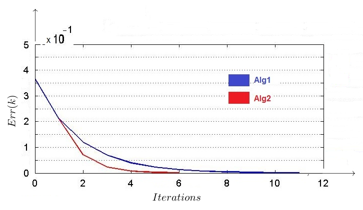
Here, the error function can be defined by $Err(k)=\Vert x_k-x^{\ast }\Vert$ at each step $k$ of the iterative method, where $x_k$ is the $k$th approximation of the solution and $x^{\ast }$ is the exact solution of the system. We indicate the value of this function at the final iteration by $Err$. For the approximate solution obtained from Algorithm 1 in the previous example, this value is $6.4613\times {10}^{-4}$, which is a little less than that of Algorithm 2 with $Err=6.5223\times {10}^{-4}$. Nevertheless, these error function values indicate that the final approximation obtained from each of our two algorithms is accurate up to four decimal places. Fig. 1 shows how Algorithm 1 and Algorithm 2 converge to the exact solution of the system in Example 6.

Although the Richardson iterative method is a light calculation method that is used in many applications of iterative methods in the solution of linear systems, our examples show that in many cases, the number of iterations required to reach the desired solution in Richardson’s method is greater than that of our second method. For instance, in the following example and the special case $ϵ=0.001$, the number of iterations required in Richardson’s method is equal to $30322$ and the final error value is equal to $Err=2.1836\times {10}^{-4}$. But, in our second algorithm, this number is equal to $23896$ with an error value equal to $Err=1.2679\times {10}^{-4}$.

Example 7.

Let

It is straightforward to investigate that $D$ is invertible and self-adjoint. Assuming

$$f=\left[\begin{array}{c}0.1\\ 2\\ 8\end{array}\right],$$

$c_1=0.2918$ and $c_2=13556700$, the following results are obtained for the system $Dx=f$ .

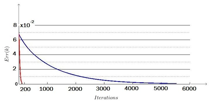
The maximum error for the approximate solution of this system is $Err=2.4138$. For the case $ϵ=0.01$, Richardson’s method obtains the approximate solution after $22893$ iterations with time $t=0.084436$ $sec.$ and $Err=0.0057$, but for Algorithm 2, these numbers are $18747$ iterations with $t=0.301137$ and $Err=0.0024$. In this case, Algorithm 1 works slowly but finally converges to the exact solution of the system. Here, the CG method does not work at all.

The optimal values for $c_1$ and $c_2$ in the previous example are ${\lambda }_{\min }(D^2)=0.3090$ and ${\lambda }_{\max }(D^2)=13556690$. As can be seen, in this example, there is no need to use optimal values for $c_1$ and $c_2$. Table 2 presents the numerical results of the iterations required to converge to the exact solution of the systems in Example 7.

	$0.01$	$0.001$	$0.0001$
The Richardson algorithm	$22893$	$30322$	$37968$
Algorithm 1	$>1million$	$>1.5million$	$>2.5million$
Algorithm 2	$18747$	$23896$	$29038$
The CG algorithm	No Respond	No Respond	Not Respond

Table 2. The number of iterations needed to converge to $x^{\ast }$ for the Richardson iterative method, Algorithm 1, Algorithm 2 and the CG method in Example 7, for $ϵ=0.01,0.001$ and $0.0001$.

As shown in Table 2, in this special example, the well-known method CG does not work at all, while our first algorithm works, although slowly!

Also, we can see in Table 2 that the required number of iterations with different values of $ϵ$ in Algorithm 2 is less than that of Richardson’s method.

According to the above example, if we ignore the condition of positive definiteness, then the algorithm of the Conjugate Gradient method fails to work. Moreover, if the matrix of the system has negative eigenvalues, then the Richardson iterative method fails to work either. The following examples illustrate such systems.

	$0.01$	$0.001$	$0.0001$
The Richardson algorithm	No Respond	No Respond	No Respond
Algorithm 1	$2$	$58$	$115$
Algorithm 2	$2$	$11$	$19$
The CG algorithm	No Respond	No Respond	No Respond

Table 3. The number of iterations needed to converge to $x^{\ast }$ for the Richardson iterative method, Algorithm 1, Algorithm 2 and the CG method in Example 8, for $ϵ=0.01,0.001$ and $0.0001$.

	$0.01$	$0.001$	$0.0001$
The Richardson algorithm	No Respond	No Respond	No Respond
Algorithm 1	$0.000033$	$0.000329$	$0.000674$
Algorithm 2	$0.000171$	$0.000263$	$0.000391$
The CG algorithm	No Respond	No Respond	No Respond

Table 4. The run-time of the Richardson iterative method, Algorithm 1, Algorithm 2 and the Conjugate Gradient method in seconds for $ϵ=0.01,0.001$ and $0.0001$ in Example 8.

Example 8.

Assume that

and

$$f=\left[\begin{array}{c}-8\\ 25\\ 14\end{array}\right]$$

then the eigenvalues of $D$ are negative. Therefore the parameter $\alpha$ in Richardson’s method is negative so it will not work for solving the system $Dx=f$. But in this case, with $c_1={\lambda }_{\min }(D^2)=8122414$ and $c_2={\lambda }_{\max }(D^2)=799751706$, both our two algorithms lead to the approximated solution for the system properly.

In addition, due to the non-definite positivity of $D$, the CG method does not respond.

Table 3 shows detailed information about the required iterations to converge to the exact solution of the system by using different tolerance thresholds $ϵ$. Also, a summary of the obtained information about the runtime of our algorithms is given in Table 4.

Algorithms	Number of iterations	Run-time	$Err$
Algorithm 1	$60$	$0.000741$	$5.894\times {10}^{-4}$
Algorithm 2	$12$	$0.000277$	$6.8232\times {10}^{-4}$

Table 5. Run-time, number of iterations and final error $Err$ needed for Algorithm 1 and Algorithm 2 to converge, by using perturbed values $c_1=7923000$ and $c_2=799841230$ in Example 8 for $ϵ=0.001$.

Algorithms	Number of iterations	Run-time	$Err$
Algorithm 1	$12$	$0.222026$	$5.0480\times {10}^{-4}$
Algorithm 2	$6$	$0.007273$	$5.0355\times {10}^{-4}$

Table 6. Run-time, number of iterations, and final error $Err$ needed for Algorithm 1 and Algorithm 2 to converge using perturbed values $c_1=3698$ and $c_2=27918$ in Example 9 for $ϵ=0.001$.

In Fig. 2, we show the way our algorithms converge to the exact solution during successive iterations. We use the broken-line diagram to compare the convergence of our algorithms at each step $k$. As seen in Fig. 2, Algorithm 2 converges faster than Algorithm 1. Also, the CG algorithm operates at only one step and fails to converge. Note that this diagram corresponds to the error threshold $ϵ=0.001$.

Here is another example in which Richardson’s method fails to converge due to a negative parameter $\alpha$.

Example 9.

Suppose that in the linear system $Ax=y$, the matrix of $A$ is given by

and

$$y=\left[\begin{array}{c}8\\ -22\\ 10\end{array}\right].$$

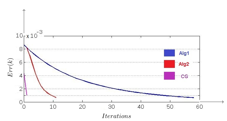
Then, ${\lambda }_{\min }(A)=-168.6671$ and ${\lambda }_{\max }(A)=-53.8876$. So, and this means that the Richardson iterative method fails to converge in this case. The maximum error of the approximate solution is equal to the norm of the exact solution, which is $0.3623$. Let $ϵ=0.001$. Then, by using $c_1={\lambda }_{\min }(A^2)=3766.2$ and $c_1={\lambda }_{\max }(A^2)=27404$, Algorithm 1 converges in $16$ steps with final error $Err=1.8055\times {10}^{-4}$. Also, Algorithm 2 converges in $8$ steps, and its final error is $Err=1.8868\times {10}^{-4}$. This value equals $Err=0.0074$ for the CG method, which is greater than the threshold $ϵ=0.001$. Thus, in this case, the CG method fails to converge and operates only one step. Fig. 3 compares the convergence speeds of our algorithms with each other and with the Conjugate Gradient method in this example.

To demonstrate that an approximation of the optimal values $c_1$ and $c_2$ suffices for both our algorithms, we have obtained approximated values for $c_1$ and $c_2$ in the two examples above applying eigenvalue approximation methods, particularly the Power Method [13]. We then re-executed Example 8 and Example 9 using these approximations with a tolerance of $ϵ=0.001$. The results are summarized in Table 5 for Example 8 and Table 6 for Example 9.

As illustrated in Table 5 and Table 6, our algorithms exhibit favorable performance when utilizing the approximate values of $c_1$ and $c_2$.

Figure 2. The graph of the error function $Err(k)$ concerning iteration step $k$ for Algorithm 1, Algorithm 2, and CG algorithm in Example 8.

Figure 3. The graph of the error function $Err(k)$ concerning iteration step $k$ for Algorithm 1 and Algorithm 2 in Example 9.

Example 10.

Let $A$ be the following matrix,

that is a finite difference discretization of the Laplace PDE of dimension 150 [11], and . Then $A$ is self-adjoint and invertible but not positive definite, hence in this case CG method does not work at all. Since eigenvalues of $A$ are all negative, the Richardson method cannot be applied. But our first method converges in $t=334.3829$ seconds at $239591$ steps and our second algorithm converges to the solution of the system $Ax=y$ in just $1417$ iterations within $23.09$ seconds with final error $Err=7.8411\times {10}^{-4}$ for $ϵ=0.001$. This final error for our first algorithm is $Err=7.7815\times {10}^{-4}$.

Here, $c_1=1.8735\times {10}^{-7}$ and $c_2=15.9965$ are optimal values satisfying in equation (3).

5. Conclusions

In this paper, we proposed two new iterative methods for solving an operator equation $Ax=y$, with $A$ being bounded, self-adjoint, and positive definite. Our first method used an iterative relation with a convergence rate equal to ${\left(\frac{{\lambda }_{\max }(A^2)-{\lambda }_{\min }(A^2)}{{\lambda }_{\max }(A^2)-{\lambda }_{\min }(A^2)}\right)}^2$ and the second method used the Chebyshev polynomials to accelerate the convergence rate of the first method.

Although the Richardson and Conjugate Gradient methods are among the most popular methods used in various applications, they are inefficient for a wide range of linear systems. Our algorithms worked decently well in such cases. Both the Richardson and Conjugate Gradient methods have limitations in their fields of application. For instance, Richardson’s algorithm is limited by the assumption that the parameter $\alpha$ is positive, and so, fails to work if $\alpha \le 0$. Nevertheless, our algorithms worked properly in most of these cases. Meanwhile, our second iterative method needed fewer iterations than Richardson’s method to converge. Also, the positive definiteness of the operator is an essential condition for the CG method, and the method fails to respond if the system’s operator $Ax=y$ is not positive definite. However, our algorithms can converge if the operator is only invertible and self-adjoint.

Since iterative methods have various applications in other branches of science, conducting research on these methods and their development can greatly help other researchers in different scientific fields. We hope that this work will motivate researchers to develop such methods and help other researchers in the field of numerical solutions of linear systems.

References

- [1]
- [2] S.F. Ashby, T.A. Manteuffel and J.S. Otto, A comparison of adaptive Chebyshev and least squares polynomial preconditioning for Hermitian positive definite linear systems, SIAM J. Sci. Statist. Comput., 13 (1992), pp. 1–29. https://doi.org/10.1137/0913001
- [3] C.C. Cheny, Introduction to Approximation Theory, McGraw Hill, New York, 1996.
- [4] S. Dahlke, M. Fornasier and T. Raasch, Adaptive frame methods for elliptic operator equations, Advances in comp. Math., 27 (2007), pp. 27–63.
- [5] I. Daubechies, G. Teschke and L. Vese, Iteratively solving linear inverse problems under general convex constraints, Inverse Probl. Imaging, 1 (2007), pp. 29–46.
- [6] H. Jamali and M. Kolahdouz, Using frames in steepest descent-based iteration method for solving operator equations, Sahand Commun. Math. Anal., 18 (2021), pp. 97–109. https://doi.org/10.22130/scma.2020.123786.771
- [7] H. Jamali and M. Kolahdouz, Some iterative methods for solving operator equations by using fusion frames, Filomat, 36 (2022), pp. 1955–1965. https://doi.org/10.2298/fil2206955j
- [8] H. Jamali and R. Pourkani, Using frames in GMRES-based iteration method for solving operator equations, JMMRC, 13(2023) no.2, pp. 107–119.
- [9] C.T. Kelley, A fast multilevel algorithm for integral equations, SIAM J. Numer. Anal., 32 (1995), pp. 501–513.
- [10] C.T. Kelley and E.W. Sachs, Multilevel algorithms for constrained compact fixed point problems, SIAM J. Sci. Comput., 15 (1994), pp. 645–667. https://doi.org/10.1137/0915042
- [11] R.J. LeVeque, Finite Difference Methods for Ordinary and Partial Differential Equations: Steady-State and Time-Dependent Problems, SIAM, 2007.
- [12] Y. Saad, Iterative methods for Sparse Linear Systems, PWS press, New York, 2000.
- [13] Y. Saad, Iterative methods for Sparse Linear Systems(2nd ed.), SIAM, 2011.