Controlling numerical diffusion in solving advection-dominated transport problems

Abstract.

Numerical schemes for advection-dominated transport problems are evaluated in a comparative study. Explicit finite difference methods are analyzed together with a global random walk algorithm in the frame of a splitting procedure. A robust implementation of the method of lines is also proposed as an alterative approach. The efficiency of the methods with respect to the control of the numerical diffusion is investigated numerically in one-dimensional problems with constant coefficients and two-dimensional problems with variable coefficients consisting of realizations of space-random functions.

1. Introduction

The numerical diffusion in transport problems is produced when the advection velocity is nonzero, increases with the decrease of the diffusion coefficient, and is often associated with spurious oscillations of the solution [5]. Remedies to these issues are provided by flux corrected transport and other diffusion-antidiffusion methods [2, 6], upwind schemes [7, 3], or adaptive finite volume approximations [8].

Numerical diffusion in advection-diffusion problems may be produced by the finite order of the approximations and/or by numerically induced smoothing. In such circumstances, a small amount of numerical diffusion may occur even when the velocity vanishes [2, 9]. But above all, the numerical diffusion cannot be avoided when stabilizing upwind schemes are used to prevent oscillations of the numerical solution [9]. To illustrate this situation let us consider the advection equation,

$$\frac{\partial c}{\partial t}+V\frac{\partial c}{\partial x}=0,$$

and the finite difference (FD) scheme with upwind space discretization,

$$\frac{c_{i,k+1}-c_{i,k}}{\mathrm{\Delta }t}+V\frac{c_{i,k}-c_{i-1,k}}{\mathrm{\Delta }x}=0,$$

which provides solutions at $x=i\mathrm{\Delta }x$ and $t=k\mathrm{\Delta }t$ according to the recurrent relation

$$c_{i,k+1}=(1-Cr)c_{i,k}+Cr{c}_{i-1,k},$$

where $Cr=V\mathrm{\Delta }t/\mathrm{\Delta }x$ is the Courant number.

Performing Taylor expansions of $c_{i,k+1}$ and $c_{i-1,k}$ (in $\mathrm{\Delta }t$ and $\mathrm{\Delta }x$, respectively) one obtains [4].

$$\frac{\partial c}{\partial t}+V\frac{\partial c}{\partial x}=\frac{1}{2}V\mathrm{\Delta }x(1-Cr)\frac{{\partial }^{2}c}{\partial x^2}+\text{higher order terms}.$$

The above relation shows that the FD scheme is unstable for Courant number $Cr>1$ [11, Sect. 2.2], the scheme is stable but diffusive for , and there is no numerical diffusion for $Cr=1$. A small $(1-Cr)>0$ ensures that the scheme produces only a small amount of numerical diffusion.

Although, in general, discrete error norms used to measure differences from reference solutions do not discriminate between different sources of errors (e.g., discretization, truncation, numerical diffusion) a quantification of the numerical diffusion is sometimes obtained, for nonsteady transport problems, by using the spatial moments of the solution [6, 9]. For constant velocity and diffusion coefficients, it was found that the diffusion coefficient estimated from the second central spatial moment of the concentration computed with different numerical schemes (linear and quadratic finite element methods with and without upwind, different mixed-finite element implementations, and finite volume methods) is affected by errors of the order of the nominal diffusion coefficient, which can hardly be reduced by refining the discretization for mesh Péclet numbers $\ge 1$ [9, Tables 1-8]. In case of diffusion in random velocity fields simulations of transport in groundwater, the differences between the effective dispersion coefficients estimated by these methods and those obtained by global random walk (GRW) simulations, free of numerical diffusion, can be even larger [9, Figs. 5-10].

2. One-dimensional advection-diffusion process with constant coefficients

The advection-diffusion process used in the following to test one-dimensional (1D) numerical schemes is governed by the parabolic equation with constant coefficients

(1) $${\partial }_{t}c+V_0{\partial }_{x}c=D_0{\partial }_{xx}c,$$

with analytical solution given by the normalized Gaussian function

(2) $$c(x,t)={(4\pi D_{0}t)}^{-1/2}\exp \left[-(x-x_0-V_{0}t)/(4D_{0}t)\right].$$

The constant coefficients in Eq. (1) are chosen as $V_0=1$ m/d and $D_0=0.01$ m²/d. These coefficients are representative for a typical numerical setup for transport in groundwater [9, 12]. (Hereafter, all spatial and temporal dimensions are given in meters and days, respectively.) In this section, we compare solutions obtained by several numerical schemes of the Cauchy problem for Eq. (1) in the domain $(0,L)\times [0,T]$, $L=300$, $T=200$, for the initial condition given by the analytical solution (2) evaluated at $t=1$ for $x_0=1$ and normalized by its spatial integral over the interval $(0,L)$. The length $L$ of the spatial interval was large enough to contain the support of the numerical solution at the final time $T$. The left/right boundary conditions are thus $c(0,t)=c(L,t)=0$.

Accuracy estimates are done by comparisons of the numerical solution $c^{num}$ with the analytical solution $c$, as well as by comparisons with the nominal parameters $V_0$ and $D_0$ of the velocity $V=M_1/t$ and the diffusion coefficient $D=(M_2-M_1^2)/(2t)$ computed from the first two spatial moments of the numerical solution, $M_1$ and $M_2$, respectively. The spatial moments are averages weighted by the numerical solution normalized to unity, $c_{i,k}$, $i=1,\mathrm{\dots },L/\mathrm{\Delta }x$, $k=1,\mathrm{\dots },T/\mathrm{\Delta }t$, where $\mathrm{\Delta }x$ and $\mathrm{\Delta }t$ are discretization steps, computed by relations of the form

(3) $$M_{\alpha }(k\mathrm{\Delta }t)=\sum _{i=1}^{L/\mathrm{\Delta }x}{(x-x_0)}^{\alpha }{c}_{i,k},\alpha =1,\mathrm{\hspace{0.33em}2}.$$

2.1. Global random walk and equivalent finite difference schemes

The 1D GRW algorithm approximates the solution of (1) by $c^{num}\approx n_{j,k}$, where $n_{j,k}$ are numbers of particles at the sites of a regular lattices moving according to the random walk rule [15]. Groups of $n(j,k)$ particles lying at the sites $j$ of the 1D lattice are scattered at the time step $k$, and the particle distribution is updated at $k+1$, according to

(4) $n(j,k)=\delta n_{j+v_j,j,k}+\delta n_{j+v_j-d,j,k}+\delta n_{j+v_j+d,j,k},$

(5) $n(i,k+1)=\delta n_{i,i,k}+{\displaystyle \sum _{j\ne i}}\delta n_{i,j,k},$

where the amplitude of the diffusion jumps $d$, the space step $\mathrm{\Delta }x$, and the time step $\mathrm{\Delta }t$ are related by , which ensures that the numerical solution is free of numerical diffusion [12, 13], and $v_j=round(V_j\mathrm{\Delta }t/\mathrm{\Delta }x),|v_j|\ge 1$ is the dimensionless velocity. Note that $|v_j|$ is an integer Courant number ($Cr$). The ensemble averages of the quantities $\delta n$ in relations (4)-(5) are given by the random walk rules

(6) $$\overline{\delta n_{j+v_j\pm d,j,k}}=\frac{1}{2}r\overline{n_{j,k}},\overline{\delta n_{j,j+v_j,k}}=(1-r)\overline{n_{j,k}}.$$

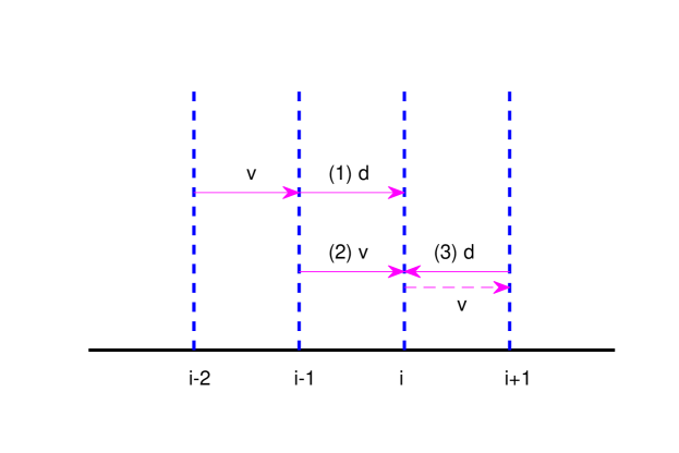
Giving up particles indivisibility one obtains a deterministic FD scheme. Summing up the contributions (5) to $n_{i,k+1}$ coming from diffusive jumps (d) and displacements due to velocity field (v), according to (4) (for $v=d=1$), respectively (1)d, (2)v, and (3)d shown in Fig. 1, one obtains the explicit FD scheme

(7) $$n_{i,k+1}=(1-r)n_{i-1,k}+\frac{r}{2}(n_{i-2,k}+n_{i,k}).$$

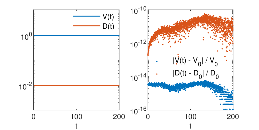
Fig. 2 shows that the velocity $V$ and the diffusion coefficient $D$ computed, according to (3), from the spatial moments of the GRW-FD solution (7) provide highly accurate estimations of the constant coefficients $V_0$ and $D_0$ of the advection-diffusion equation (1).

Figure 1. Illustration of GRW-FD scheme (7).

Figure 2. Velocity and diffusion coefficient estimated from the fist two spatial moments of the numerical solution $n_{i,k}$ obtained with the GRW-FD scheme (left) and the relative errors with respect to the nominal values of $V_0$ and $D_0$ in Eq. (1) (right).

The FD scheme (7) is equivalent to a splitting FD scheme with the following advection (a) and diffusion (d) steps:

(8) $n_{i,k+1/2}^a$ $=$ $n_{i-1,k},$

(9) $n_{i,k+1}^d$ $=$ ${\displaystyle \frac{r}{2}}{n}_{i-1,k+1/2}^a+{\displaystyle \frac{r}{2}}{n}_{i+1,k+1/2}^a+(1-r)n_{i,k+1/2}^a.$

The advection scheme (8) is the discrete version of the exact solution of the advection equation, $c(x,t+\mathrm{\Delta }t)=c(x-V_0\mathrm{\Delta }t,t)$. The diffusion scheme (9) is the stable explicit forward-time central-space FD scheme for the heat equation,

$$\frac{n_{i,k+1}-n_{i,k}}{\mathrm{\Delta }t}=D\frac{1}{\mathrm{\Delta }x}\left(\frac{n_{i+1,k}-n_{i,k}}{\mathrm{\Delta }x}-\frac{n_{i,k}-n_{i-1,k}}{\mathrm{\Delta }x}\right).$$

Since the dimensionless velocity has to be an integer greater than unity, the GRW splitting-scheme (8)-(9) is defined for integer Courant numbers $Cr\ge 1$.

One remarks that the GRW-advection scheme (8) is a particular case, for Courant number $Cr=1$, of the upwind (UPW) scheme

(10) $$n_{i,k+1}=n_{i,k}-Cr(n_{i,k}-n_{i-1,k}),$$

and of the BOX scheme

(11) $$n_{i,k+1}=n_{i-1,k}+[(1-Cr)/(1+Cr)](n_{i,k}-n_{i-1,k+1}).$$

While the UPW scheme is stable only if $Cr\le 1$, the BOX scheme is unconditionally stable [11]. However, since (11) is an implicit scheme, for an easier implementation and to achieve faster computations, we use in the following a linearized version consisting of replacing $n_{i-1,k+1}$ by $n_{i-1,k}$. As we will see in Section 2.3, this linearized BOX scheme is no longer unconditionally stable.

The solution of these three schemes is obtained with the same Matlab code by choosing the advection scheme (8) for GRW, (10) for UPW, (11) for BOX, while using the same scheme (9) for the diffusion step.

2.2. Method of Lines

The Method of Lines (MOL) is an effective numerical technique for solving partial differential equations (PDEs), particularly useful in advection-dominated transport problems. This method discretizes the spatial domain while preserving the time domain as continuous, thereby transforming the PDE into a system of ordinary differential equations (ODEs). These ODEs are subsequently solved using established ODE solvers, providing a robust framework for addressing the challenges inherent in advection-dominated scenarios. For more details on the MOL, consult [10].

If we consider a discretization with $N$ grid points with spacing $\mathrm{\Delta }x$: $x_i=x_0+i\mathrm{\Delta }x,i=0,1,2\mathrm{\dots },N$ then the spatial derivatives ${\partial }_{x}c$ and ${\partial }_{xx}c$ can be approximated at each grid point with a FD scheme.

For improved accuracy, higher-order FD approximations can be derived using Taylor series expansions. The derivation is achieved by combining multiple Taylor series expansions at different points such that the lower-order terms cancel out, leaving higher-order terms as the dominant source of error.

In the following, we use the central-space FD approximation

(12) $${\partial }_{x}c|{}_{x=x_i}\approx \frac{c_{i+1}-c_{i-1}}{2\mathrm{\Delta }x},$$

where $c_i$ denotes the value of $c$ at the $i$-th grid point. Similarly, we consider the central-space approximation of the second derivative,

(13) $${\partial }_{xx}c|{}_{x=x_i}\approx \frac{c_{i+1}-2c_i+c_{i-1}}{\mathrm{\Delta }{x}^2}.$$

Substituting the FD approximations (12) and (13) into Eq.(1) transforms it into a system of ODEs:

(14) $${\partial }_t{c}_i=-V_0\frac{c_{i+1}-c_{i-1}}{2\mathrm{\Delta }x}+D_0\frac{c_{i+1}-2c_i+c_{i-1}}{\mathrm{\Delta }{x}^2},1\le i\le N.$$

Since Eq. (14) constitutes $N$ first-order initial-value ODEs, $N$ initial conditions are required, which are generated from the reference solution (2) at the initial time $t=1$.

In the system of ODE (14) we have $N$ equations with $N+2$ unknown functions. The solution at $x_0$ satisfies the Dirichlet boundary condition. Consequently, $c_0$ is already known and can be substituted into the system of equations accordingly. At $i=N$ the function $c_{N+1}$ appears in the equation, which is outside the considered grid. In order to be able to reduce the number of unknowns to $N$ we must assign a value to $c_{N+1}$. Because this occurs at the boundary point $i=N$, we can obtain an approximation by using (12) and the right-boundary condition of the current numerical setup,

$${\partial }_{x}c\approx \frac{c_{N+1}-c_{N-1}}{2\mathrm{\Delta }x}=0,$$

which reduces to

$$c_{N+1}=c_{N-1}.$$

In this study, we employed the explicit fourth-order Runge-Kutta method to solve the resulting system of ODEs. We experimented with various Courant numbers to determine the threshold for significant numerical errors. With a spatial step size of $\mathrm{\Delta }x=0.1$, satisfactory results were obtained up to $Cr=2$. However, when the spatial step size was decreased to $\mathrm{\Delta }x=0.05$, the results remained accurate up to a Courant number of $2.4$.

2.3. Accuracy estimates

The accuracy of the numerical solutions presented in Fig. 3 is evaluated by the quadratic norm,

(15) $$e_c={\left(\mathrm{\Delta }x\sum _{i=1}^{L/\mathrm{\Delta }x}{\left(n_{i,k}-c(i\mathrm{\Delta }x,k\mathrm{\Delta }t)\right)}^2\right)}^{1/2}.$$

Similarly to (15), the accuracy of the estimated coefficients $V$ and $D$ is evaluated by quadratic norms on the time interval $[0,T]$ divided by the nominal coefficients $V_0$ and $D_0$. For instance, the relative error of the estimated diffusion coefficient with respect to the coefficient $D_0$,

(16) $$e_D=\frac{1}{D_0}{\left(\mathrm{\Delta }t\sum _{k=1}^{T/\mathrm{\Delta }t}{\left(D_{k\mathrm{\Delta }t}-D_0\right)}^2\right)}^{1/2},$$

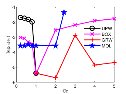
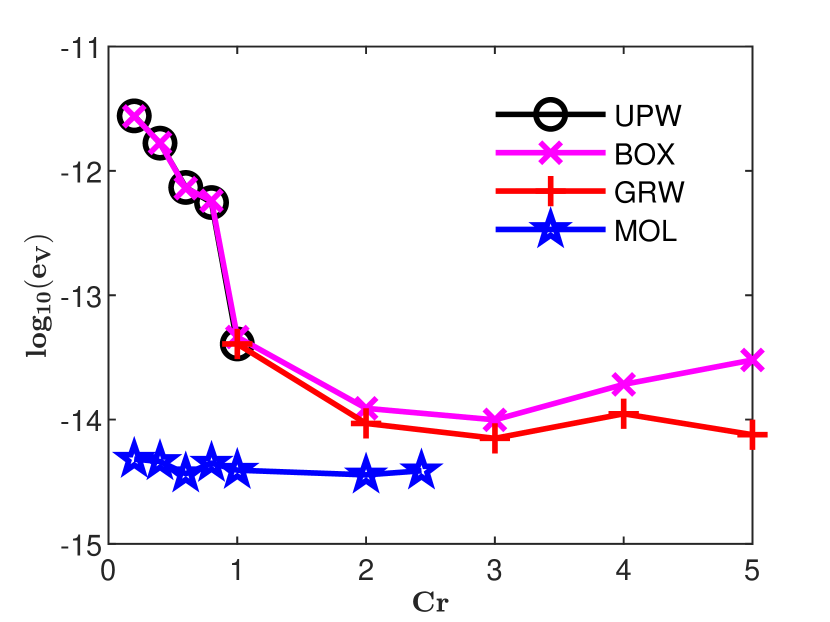
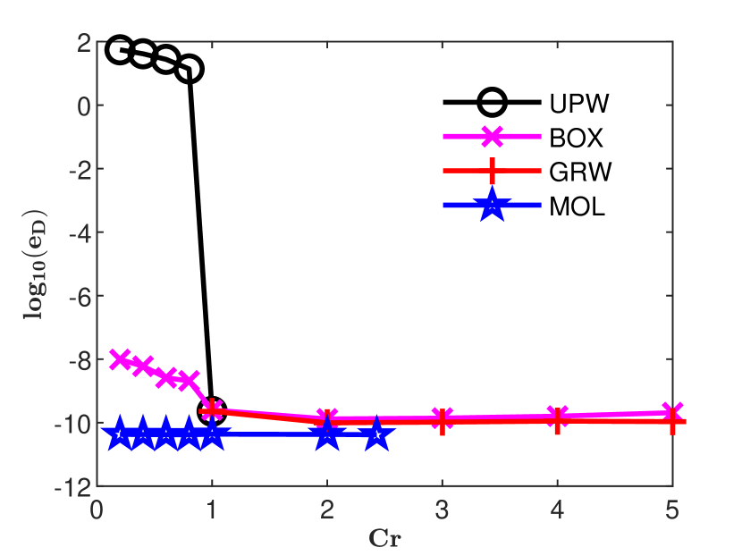
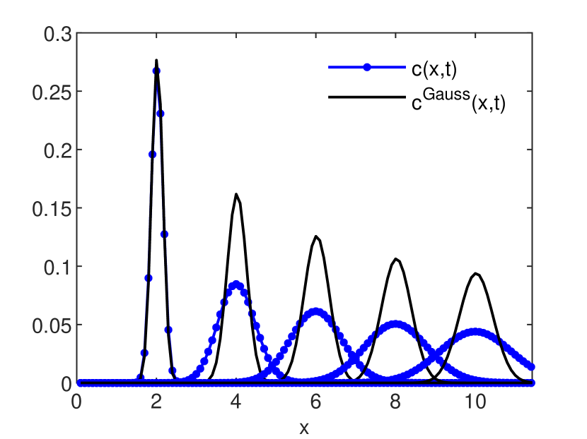
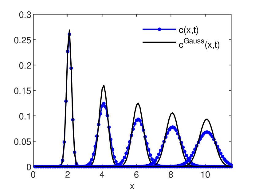
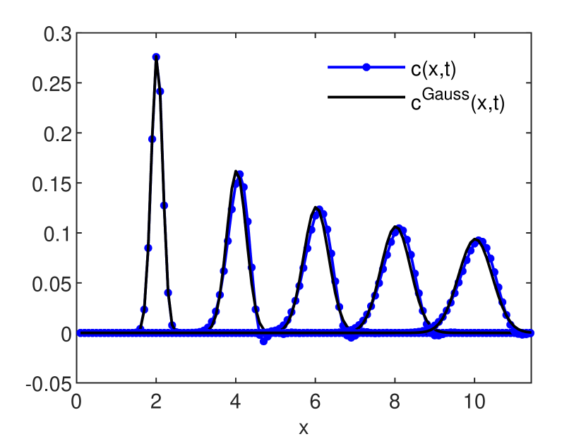
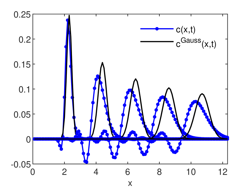
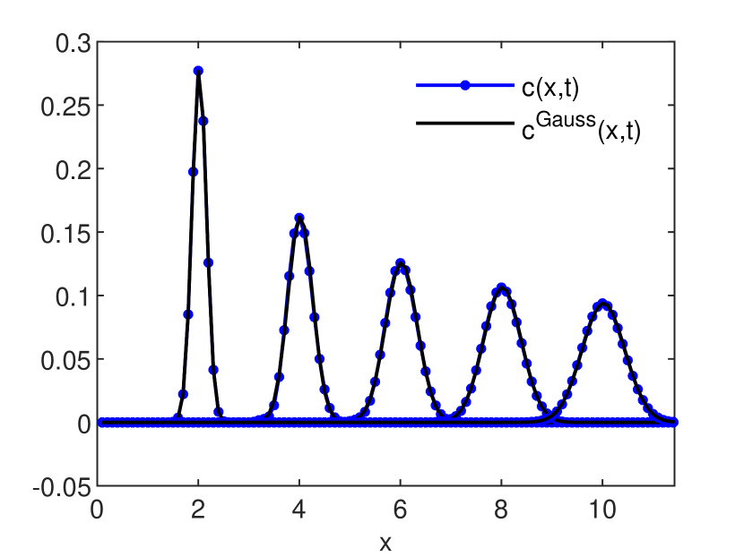
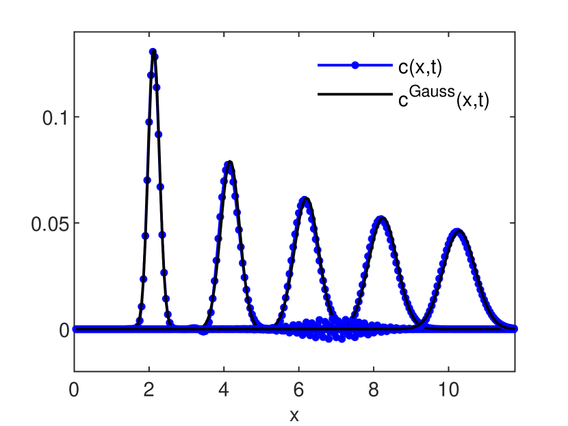
is an estimation, global in time, of the numerical diffusion (see also [6, 9]). The accuracy estimates for the GRW-FD, UPW, BOX, and MOL schemes are presented in Figs. 3 and 4. In Figs. 5, 6 and 7 the numerical solutions of the four schemes are compared to the exact Gaussian solution (2) at successive times $t\le T/20$.

Estimations (16) of numerical diffusion corresponding to the splitting GRW-FD scheme (8)-(9), UPW scheme (10), and BOX scheme (11) are presented in Fig. 4, right panel. The computations were carried out for a fixed space step $\mathrm{\Delta }x=0.1$. This corresponds to a local Péclet number $Pe=V_0\mathrm{\Delta }x/D_0=10$, that is, to an advection-dominated transport problem. The solution norms (15) were evaluated at $k\mathrm{\Delta }t=T$.

One remarks that in case $Cr=1$, when the three schemes coincide, the relative errors of the estimated coefficients from Fig. 4 are of the order ${10}^{-10}$ or smaller (see also Fig. 2), while the solution error-norm (15) from Fig. 3 is of order ${10}^{-6}$. Thus, very small relative errors of the estimated coefficients are not an appropriate indicator for the accuracy of the numerical solution. Moreover, neither of these global norms is sufficient to capture deformations of the shape of the reference solution. For instance, the significant numerical diffusion produced by the UPW scheme for , quantified by relative errors much greater than one in Fig. 4, is also observable in flattening of the numerical solution shown in Fig. 5. But, for the BOX scheme, even if acceptable errors of the solutions of at most ${10}^{-2}$ and relative errors of the coefficients smaller than ${10}^{-8}$ are obtained in all cases, the numerical solutions shown in Fig. 6 deviate from the shape of the reference solution and are affected by oscillations which grow with the departure from $Cr=1$ and are mainly significant for $Cr>1$, leading to the instability of the scheme.

As seen in Fig. 4, the GRW-FD scheme is practically free of numerical diffusion. Moreover, since the advection step (8) in the splitting procedure is the FD approximation of exact solution of the advection equation, the GRW-FD scheme reproduces almost perfectly the shape of the analytical solution, within the range of the errors shown in Fig. 3.

A special attention deserves the performance of the MOL scheme. The errors of the solution shown in Fig. 3 are of the order ${10}^{-4}$ up to $Cr\le 2$, then they grow suddenly for $Cr=2.43$ while the relative errors of the coefficients from Fig. 4 remain extremely small for the whole range $Cr\le 2.43$. At the same time, unlike the UPW and BOX FD schemes, MOL accurately reproduces the shape of the solution for all Courant numbers less then $Cr=2.55$, when the solution starts to oscillate (see Fig. 7). Therefore, MOL is much more robust than the UPW and BOX FD schemes and well suited to provide accurate solutions to advection dominated problems for moderately large Courant numbers.

Figure 3. Quadratic-norm deviations from the theoretical Gaussian with constant coefficients of numerical solutions obtained with box-, upwind-, and GRW-scheme as function of Courant number.

Figure 4. Relative errors of the velocity (left panel) and diffusion coefficient (right panel) estimated by box-, upwind-, and GRW-scheme as function of Courant number.

Figure 5. UPW scheme: comparison between numerical and reference Gaussian solution for $Cr=0.2$ (left) and $Cr=0.8$ (right).

Figure 6. BOX scheme: comparison between numerical and reference Gaussian solution for $Cr=0.2$ (left) and $Cr=3$ (right).

Figure 7. MOL: comparison between numerical and reference Gaussian solution for $Cr=0.2$ (left) and $Cr=2.55$ (right).

3. Two-dimensional diffusion with variable drift coefficients

In the following, we consider a 2D transport problem consisting of a diffusion process in a spatially variable velocity field, governed by the equation

(17) $${\partial }_{t}c+U{\partial }_{x}c+V{\partial }_{y}c=D({\partial }_{xx}c+{\partial }_{yy}c),$$

where the solution $c(x,y,t)$ represents the associated concentration field, $U$ and $V$ are drift coefficients, and $D$ is a constant diffusion coefficient.

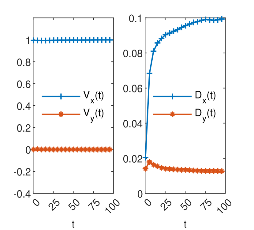
We choose $D=0.01$ and drift coefficients given by the components of a two-dimensional velocity field modeled by a fixed realization of a random space function. The latter is a linear approximation of the Darcy velocity in heterogeneous aquifers, generated by a randomization method with the Matlab function given in [13, Appendix C.3.2.2]. The hydraulic conductivity is described by a log-normal random field with Gaussian correlation, small variance ${\sigma }^2=0.1$, and correlation length $\lambda =1$. The mean velocity components are set to $⟨V_x⟩=1$ and $⟨V_y⟩=0$. The Péclet number associated to the characteristic length $\lambda$ takes a large value $Pe=U\lambda /D=100$, which indicates that the transport is dominated by advection. The effective velocity components and diffusion coefficients are computed, similarly to the 1D case, from the first two spatial moments (3) by performing a supplementary average over an ensemble of realizations of the velocity field according to

(18) $$V_x=⟨M_{1x}⟩/t,D_x=⟨M_{2x}-M_{1x}^2⟩/(2t),$$

and similarly for $V_y$ and $D_y$. For the parameters specified above, the effective velocity components are constant and coincide with their ensemble averages and the effective diffusion coefficients evolve asymptotically in time towards $D_x=D+U{\sigma }^2\lambda =0.1$ and $D_y=D=0.01$ [14, Sect. 4.1].

Fig. 9 shows a numerical solution of Eq. (17) with the above parameters, obtained by repeating the 1D GRW procedure (4)-(6) in both spatial directions. Estimations of the effective coefficients (18) for the same problem are presented in Fig. 9.

Figure 8. Distribution of $N={10}^{24}$ particles at successive steps in a two-dimensional GRW simulation.

Figure 9. Effective velocity components and diffusion coefficients estimated from an ensemble of 1000 GRW solutions.

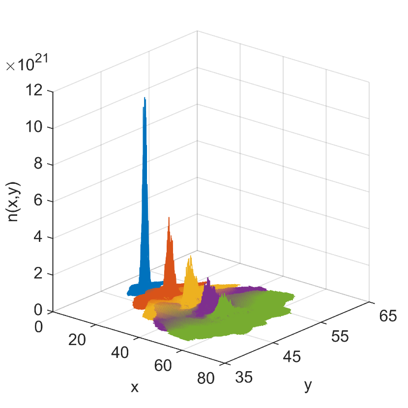
The numerical schemes evaluated in the following solve Eq. (17) in a spatial domain $(0,L_x)\times (0,L_y)$ and a time interval $(0,T)$. For fixed $T=10$, the longitudinal and transverse lengths of the spatial domain, $L_x=20$ and $L_y=12$, are large enough to ensure that the support of the concentration field does not reach the boundaries until the end of simulations. The initial condition is an instantaneous Dirac pulse at $x_0=Lx/10$ and $y_0=L_y/2$ and the numerical solutions are normalized to unity. For instance, in GRW simulations, the initial condition consists of a pulse of $N={10}^{24}$ particles released at $(x_0,y_0)$ and the normalized concentration is given by $n(x,y)/N$.

3.1. Biased GRW algorithm

The biased-GRW algorithm (BGRW) accounts for the advective terms in Eq. (17) by increasing the probability that a random walker takes a jump in the flow direction and decreasing the jump probability in the opposite direction.

The two-dimensional BGRW is defined by the relation

(19) $n_{i,j,k}$ $=$ $\delta n_{i,j\mid i,j,k}$

$+$ $\delta n_{i+1,j\mid i,j,k}+\delta n_{i-1,j\mid i,j,k}$

$+$ $\delta n_{i,j+1\mid i,j,k}+\delta n_{i,j-1\mid i,j,k},$

where $n_{i,j,k}$ is the number of particles at the site $(x,y)=(i\mathrm{\Delta }x,j\mathrm{\Delta }y)$ at the time $t=k\mathrm{\Delta }t$ and the $\delta n$ are binomial random variables describing the number of particles waiting at the initial lattice site or jumping to the first-neighbor sites. To the drift (velocity) and diffusion coefficients of the transport problem, $U(x,y,t)$, $V(x,y,t)$, and $D$, one associates the dimensionless parameters,

(20) $$u_i=U\frac{\mathrm{\Delta }t}{\mathrm{\Delta }x},v_j=V\frac{\mathrm{\Delta }t}{\mathrm{\Delta }y},r_i=D\frac{2\mathrm{\Delta }t}{\mathrm{\Delta }{x}^2},r_j=D\frac{2\mathrm{\Delta }t}{\mathrm{\Delta }{y}^2}.$$

Instead of the unbiased GRW rule (6), the average numbers of jumps in the BGRW algorithm (19) are now given by

$\overline{\delta n_{i,j\mid i,j,k}}=(1-r_i-r_j)\overline{n_{i,j,k}},$

$\overline{\delta n_{i\pm 1,j\mid i,j,k}}={\displaystyle \frac{1}{2}}(r_i\pm u_i)\overline{n_{i,j,k}},$

(21) $\overline{\delta n_{i,j\pm 1\mid i,j,k}}={\displaystyle \frac{1}{2}}(r_j\pm v_j)\overline{n_{i,j,k}}.$

As follows from (21), the BGRW algorithm is subject to the following restrictions

(22) $$r_i+r_j\le 1,\left|v_i\right|\le r_i,\left|v_j\right|\le r_j.$$

By the last two inequalities in (22), the Courant numbers $|V_x|\mathrm{\Delta }t/\mathrm{\Delta }x$ and $|V_y|\mathrm{\Delta }t/\mathrm{\Delta }y$ are smaller than one, which ensures that the BGRW algorithm is free of overshooting errors. If, in addition, one imposes the conditions $r_i\le 0.5$ and $r_j\le 0.5$, the von Neumann’s criterion for stability is also satisfied, which implies the lack of numerical diffusion and the convergence of order $𝒪(\mathrm{\Delta }{x}^2)$ of the BGRW algorithm (19), interpreted as a FD scheme, is implied by the Lax-Richtmyer Equivalence Theorem [11]. The BGRW solutions will be used in the following as reference to evaluate the unbiased GRW algorithm.

3.2. Unbiased GRW scheme

Since the diffusion coefficient is constant, the unbiased GRW solutions to the transport problem formulated in the beginning of this section are obtained in two steps, first by performing the 1D GRW procedure (4)-(6) in the $x$-direction, then by applying the same procedure to the output of the first step in the $y$-direction [15, 12, 13].

Figure 10. Relative errors of the velocity (left panel) and diffusion coefficient (right panel) estimated from a single GRW solution with respect to the corresponding coefficients obtained from a single BGRW solution.

Figure 11. Relative errors of the velocity (left panel) and diffusion coefficient (right panel) estimated from an ensemble of 100 GRW solutions with respect to the corresponding coefficients obtained from an ensemble of 100 BGRW solutions.

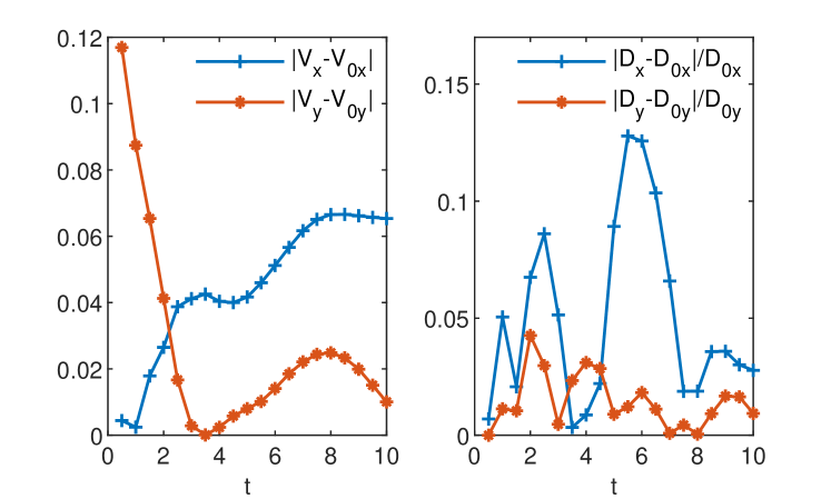
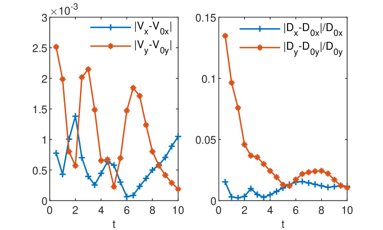
Errors of GRW estimates of the effective coefficients for a single realization of the random velocity field are presented in Fig. 10 and errors of the ensemble averaged coefficients (18) are presented in Fig. 11. For a fixed realization of the velocity field (Fig. 10) the relative errors of the unbiased GRW scheme range from a few percents to more than $10\%$. This is due to the overshooting produced when there are significant variations of the velocity over the advective displacements $u_i$ and $v_j$ which encompass several grid points in the unbiased GRW algorithm. However, the overshooting errors are smoothed out by the ensemble averaging and the results provided by the unbiased GRW scheme become closer and closer to those of the BGRW scheme as the transport process progresses in time (Fig. 11). This validates the unbiased GRW scheme, which is faster, since not constraint by $Cr\le 1$, as an efficient tool for large scale simulations of transport in random velocity fields.

4. Conclusions

The numerical diffusion in advection-dominated problems can be directly estimated by comparing the diffusion coefficient derived from the spatial moments of the numerical solution to the nominal coefficient. However, since this is a global estimate, it does not guarantee that the numerical scheme accurately reproduces the shape of the exact solution of the transport problem.

In this study, we compared the performance in solving the one-dimensional advection-diffusion equation with constant coefficients of two classical FD schemes, UPW and BOX, an unbiased GRW scheme, and a MOL scheme. For Courant number $Cr=1$, the FD and the GRW schemes coincide. In this case, they produce a negligible amount of numerical diffusion and do not deform the shape of the exact solution. Instead, for $Cr\ne 1$ the shape of the solutions of the FD schemes may deviate significantly from that of the exact solution even if the numerical diffusion is negligible.

The GRW scheme is by construction free of numerical diffusion. Additionally, since it performs advective displacements according to the exact solution of the advection equation, the unbiased GRW scheme preserves the shape of the exact solution for any integer $Cr\ge 1$. The MOL scheme is free of numerical diffusion as well and reproduces the shape of the exact solution for all Courant numbers $Cr\le 2.43$.

For the purpose of practical applications for two-dimensional simulations of transport in groundwater, the unbiased GRW has been evaluated through comparisons with the BGRW scheme, which simulates advection by using biased jump probabilities. The BGRW scheme is highly accurate but much slower than the unbiased scheme. The unbiased GRW is faster because it is not not constraint by small Courant numbers, but, for the same reason, it is less accurate due to the overshooting errors. However, the average over an ensemble of realizations of the random velocity field, which model the heterogeneity of the aquifer system, reduces the effect of the overshooting and the unbiased GRW scheme is an efficient tool for assessing statistical inferences on the transport process.

References

- [1]
- [2] D.L. Book, C. Li, G. Patnaik and F.F. Grinstein, Quantifying residual numerical diffusion in flux-corrected transport algorithms, J. Sci. Comp. 6(3) (1991), 323–243. https://dx.doi.org/10.1007/BF01062816
- [3] F. Brunner, F.A. Radu, M. Bause M and P. Knabner, Optimal order convergence of a modified BDM1 mixed finite element scheme for reactive transport in porous media, Adv. Water Resour. 35 (2012), 163–171. https://dx.doi.org/10.1016/j.advwatres.2011.10.001
- [4] C.J.M. Hewett, Consistency and numerical diffusion (2021). https://www.youtube.com/watch?v=Cjb4YtgeIn0&t=263s
- [5] P. Knabner and L. Angermann, Numerical methods for elliptic and parabolic partial differential equations, Springer, New York, 2003. https://doi.org/10.1007/b97419
- [6] Kuzmin, Explicit and implicit FEM-FCT algorithms with flux linearization, J. Comput. Phys. 228(7) (2009), 2517–2534. https://dx.doi.org/doi:10.1016/j.jcp.2008.12.011
- [7] D. Kuzmin, A. Hannukainen and S. Korotov, A new a posteriori error estimate for convection-reaction-diffusion problems, J. Comput. Appl. Math. 218(1) (2008), 70–78. https://dx.doi.org/10.1016/j.cam.2007.04.033
- [8] M. Ohlberger and C. Rohde, Adaptive finite volume approximations of weakly coupled convection dominated parabolic systems, IMA J. Numer. Anal. 22(2) (2002), 253–280. https://dx.doi.org/10.1093/imanum/22.2.253
- [9] F.A. Radu, N. Suciu, J. Hoffmann, A. Vogel, O. Kolditz, C-H. Park and S. Attinger, Accuracy of numerical simulations of contaminant transport in heterogeneous aquifers: a comparative study, Adv. Water Resour. 34 (2011), 47–61. https://dx.doi.org/10.1016/j.advwatres.2010.09.012
- [10] W.E. Schiesser and G.W. Griffiths, A compendium of partial differential equation models: method of lines analysis with Matlab, Cambridge University Press, 2009. https://doi.org/10.1017/CBO9780511576270
- [11] J.C. Strikwerda, Finite Difference Schemes and Partial Differential Equations, SIAM, 2004. https://doi.org/10.1137/1.9780898717938
- [12] N. Suciu, Diffusion in random velocity fields with applications to contaminant transport in groundwater, Adv. Water Resour. 69 (2014) 114-133. http://dx.doi.org/10.1016/j.advwatres.2014.04.002
- [13] N. Suciu, Diffusion in Random Fields. Applications to Transport in Groundwater, Birkhäuser, Cham, 2019. https://doi.org/10.1007/978-3-030-15081-5
- [14] N. Suciu, L. Schüler, S. Attinger and P. Knabner, Towards a filtered density function approach for reactive transport in groundwater, Adv. Water Resour. 90 (2016), 83–98. https://dx.doi.org/10.1016/j.advwatres.2016.02.016
- [15] C. Vamoş, N. Suciu and H. Vereecken, Generalized random walk algorithm for the numerical modeling of complex diffusion processes, J. Comput. Phys., 186 (2003), 527–544. https://doi.org/10.1016/S0021-9991(03)00073-1