Exponential B-spline collocation Method
for Singularly Perturbed Time-fractional
delay parabolic reaction-diffusion equations

Abstract.

The singularly perturbed time-fractional delay parabolic reaction-diffusion of initial boundary value problem is provided in the present study. The time-fractional derivative is applied by the Caputo fractional sense and handled by implicit Euler method. Spatial domain is handled by implementing the exponential B-spline collocation technique on Shishkin mesh. The convergence of the method is verified and has an accuracy of $𝒪(N^{-2}{(\ln N)}^2)$. In order to examine the effectiveness of the scheme three model examples are considered. The findings generated by tables and figures indicates the scheme is uniformly convergent and has dual layers at the end spatial domain.

1. Introduction

Fractional differential equations have been used to modify conventional integer order derivatives to an arbitrary (non-integer) order that can be attained in a time or space variable. It serves as great tool on assessing memory and the fundamental characteristics of various material and procedures. Fractional partial differential equations are widely employed in scientific and engineering domains, as well as numerous other fields like fluid mechanics, chemistry, viscoelasticity, finance, physics and some others [1, 2, 3, 4, 5].

Time-fractional addresses anomalous diffusion processes that are associated to time in unusual systems. Subsequently it is challenging to find analytical solutions for these sorts of issues, hence numerical approaches serve to approximate the solutions. Fractional differential equations have been the focus of a variety of computational techniques that have been devised to approximate the solution because of their capacity to simulate complicate processes [6, 7, 8].

The mathematical representation of oil reservoir simulations, flow of fluid in porous media, global water production, and several other organic occurrences have been extensively investigated using time-fractional reaction-diffusion equations [9]. Being a part of an arbitrary order causes it tricky to find the exact solutions of such issues. Finding the reliable and effective numerical approaches for such equations become increasingly crucial. Attempts at time fractional reaction-diffusion have been performed in the papers [10, 11, 12, 13].

This investigation is focused on singularly perturbed time-fractional delay parabolic reaction-diffusion of initial boundary value problems in the domain $D=D_r\times D_t=(0,1)\times (0,T];\overline{D}={\overline{D}}_r\times {\overline{D}}_t=[0,1]\times [0,T]$ and $\partial D=D-\overline{D}$:

(1) $$\left(\frac{{\partial }^{\alpha }}{\partial t^{\alpha }}-\epsilon \frac{{\partial }^2}{\partial r^2}+b(r)\right)u(r,t)+p(r,t)u(r,t-\tau )=f(r,t);(r,t)\in D$$

with the vector condition

(2) $$u(r,t)=\kappa (r,t),(r,t)\in [0,1]\times [-\tau ,0]$$

and constraints

(3) $$u(0,t)=\phi (t);u(1,t)=\varphi (t);t\in [0,T]$$

where $\epsilon$ is a small perturbation parameter which fulfills , $\tau$ is delay parameter and $b(r)\ge \vartheta >0$ is a smooth function. As soon as the functions $b(r),p(r,t),\kappa (r,t),\phi (t),\varphi (t)$, and $f(r,t))$ meet the required smoothness and compatibility requirements, the initial-boundary value problem notes a unique outcomes $u(r,t)$. This solution illustrates twin boundary layers with a thickness of $𝒪(\sqrt{\epsilon })$, that lies near the boundaries $r=0$ and $r=1$ [14, 15].

While treating parameter dependent delay parabolic reaction-diffusion issues, an order of differential equation reduces as $\epsilon \to 0$, and the differential equation solution is inevitably characterized by enormous gradient [16]. With regard to the boundary layer behavior, when employing traditional numerical techniques on a uniform mesh, substantial oscillations might strike while the perturbation parameter approaches zero over the whole areas of concern. Thus, an effective numerical method which accuracy does not depend on the perturbation parameter will be used to avoid such oscillations. In consequence, plenty of efforts have been placed into inventing numerical techniques for solving one-dimensional singularly perturbed parabolic reaction-diffusion equations with time-lag [17, 18, 19, 20, 21, 22, 23].

In [24], the theory and computation of an exponential B-spline are defined. It is commonly used in computer-aided design, surface approximation, and the curve approximations. A free parameter in exponential B-spline indicates the shape of B-spline which shows a good approximation for the data having sharp changes. A variety of differential equations are approximated by using an exponential B-spline. One of these equations involves singularly perturbed differential equations which is concerned on the studies [25, 26, 27].

Owing to author’s observation, there has been an attempts to solve integer order singularly perturbed delay differential equations using exponential B-spline approaches, however no one has successfully employed for singularly perturbed time-fractional delay parabolic reaction-diffusion equations. The present study introduces an approach for solving the initial boundary value problem of one-dimensional singularly perturbed time-fractional delay reaction-diffusion employing an exponential B-spline collocation technique on Shishkin mesh.

This investigation has a specific structure: Preliminary information and continuous solution properties are explored in Section 2. Section 3 and Section 4 consist of numerical formulation and convergence analysis, respectively. A discussion of the numerical results and conclusions are covered under Section 5 and Section 6, correspondingly.

2. Preliminaries and Properties of Continuous Solution

Definition 1.

Assume that $\mathrm{Re}(J)>0$ for any complex number $J$. The function specified by

$$\mathrm{\Gamma }(J)={\int }_0^{\mathrm{\infty }}{e}^{-r}{r}^{J-1}𝑑r$$

is a gamma function.

Definition 2.

When the function $h(t)$ possesses lowest bound of zero, then Caputo fractional derivative is described as

$$\frac{{\partial }^{\alpha }}{\partial t^{\alpha }}h(t)=\frac{1}{\mathrm{\Gamma }(k-\alpha )}{\int }_0^t{h}^{(k)}(\zeta ){(t-\zeta )}^{k-\alpha -1}𝑑\zeta ;\alpha \in (k-1,k)$$

where $h^{(k)}$ is the $k^{th}$ order derivative of $h(t)$.

Definition 3.

A function $u(r,t)$ and its Caputo fractional differentiation with regarding $t$ is described as

$$\frac{{\partial }^{\alpha }}{\partial t^{\alpha }}u(r,t)=\{\begin{array}{cc}\frac{1}{\mathrm{\Gamma }(k-\alpha )}{\int }_0^t\frac{{\partial }^{k}u(r,\zeta )}{\partial {\zeta }^k}{(t-\zeta )}^{k-\alpha -1}𝑑\zeta ;if\alpha \in (k-1,k)\hfill & \\ & \\ \frac{{\partial }^{k}u(r,t)}{\partial t^k};if\alpha =k\hfill & \end{array}$$

Lemma 4.

Let be the lowest possible value of the function $z$, where $z\in C^1[0,1]$. Then

${\partial }_C^{\alpha }z(t_0)\le \frac{t_0^{\alpha }}{\mathrm{\Gamma }(1-\alpha )}\left(z(t_0)-z(0)\right)\le 0,$

where, and ${\partial }_C^{\alpha }$ stands for the Caputo fractional derivative.

Proof.

Give an auxiliary function, $q(t)=z(t)-z(t_0)$. Then, $q(t)\ge 0$ and $q(t_0)=z(t_0)-z(t_0)=0$. Now,

$${\partial }_C^{\alpha }q(t_0)=\frac{1}{\mathrm{\Gamma }(1-\alpha )}{\int }_0^{t_0}{(t_0-\zeta )}^{-\alpha }{q}^{\prime }(\zeta )𝑑\zeta .$$

Applying integration by parts we obtain

${\partial }_C^{\alpha }q(t_0)=$ $\frac{1}{\mathrm{\Gamma }(1-\alpha )}\left(-t_0^{-\alpha }q(0)-\alpha {\displaystyle {\int }_0^{t_0}}{(t_0-\zeta )}^{-\alpha -1}q(\zeta )𝑑\zeta \right)$

$\le \frac{1}{\mathrm{\Gamma }(1-\alpha )}(-t_0^{-\alpha }q(0))$

$\le \frac{1}{\mathrm{\Gamma }(1-\alpha )}(t_0^{-\alpha }(z(t_0)-z(0)))\le 0$

∎

Given the data $b(r),p(r,t)$ and $f(r,t)$ as Holder’s continuous, and the compatibility criteria at the corner points $(0,0),(1,0),(0,-\tau )$ and $(0,\tau )$ have been met, it is shown, to ensure the existence of the unique solution for (1,2,3). That is

(4) $\kappa (0,0)$ $=\phi (0),$

$\kappa (1,0)$ $=\varphi (0),$

$\frac{{\partial }^{\alpha }\phi (0)}{\partial t^{\alpha }}$ $-\epsilon \frac{{\partial }^2\kappa (0,0)}{\partial r^2}+b(0)\kappa (0,0)+p(0,0)\kappa (0,-\tau )=f(0,0),$

$\frac{{\partial }^{\alpha }\varphi (0)}{\partial t^{\alpha }}$ $-\epsilon \frac{{\partial }^2\kappa (1,0)}{\partial r^2}+b(1)\kappa (1,0)+p(1,0)\kappa (1,-\tau )=f(1,0).$

Lemma 5.

Given that $\xi (r,t)$ is a sufficiently smooth function satisfying $\xi (r,t)\ge 0,\forall (r,t)\in \partial D$. Then, ${ℒ}_{\epsilon }\xi (r,t)\ge 0,\forall (r,t)\in D$ implies that $\xi (r,t)\ge 0,\forall (r,t)\in \overline{D}$.

Proof.

Let $(\omega ,\upsilon )$ be a point that satisfy

$$\xi (\omega ,\upsilon )=\underset{(r,t)\in \overline{D}}{\min }\xi (r,t)$$

and . Then $\xi (\omega ,\upsilon )\notin \partial D$. Then we have,

$${ℒ}_{\epsilon }\xi (\omega ,\upsilon )=\epsilon {\xi }_{rr}(\omega ,\upsilon )-b(\omega )\xi (\omega ,\upsilon )-\frac{{\partial }^{\alpha }\xi (\omega ,\upsilon )}{\partial t^{\alpha }}\le 0.$$

Since ${\xi }_{rr}(\omega ,\upsilon )\ge 0$ and $\frac{{\partial }^{\alpha }\xi (\omega ,\upsilon )}{\partial t^{\alpha }}=0$, then ${ℒ}_{\epsilon }\xi (\omega ,\upsilon )\le 0$, which contradicts the initial assumption. Thus, $\xi (\omega ,\upsilon )\ge 0$ which yields $\xi (r,t)\ge 0;\forall (r,t)\in \overline{D}$. ∎

Lemma 6.

Consider that $u(r,t)$ represents the solution to continuous problem (1). Consequently, [15]

$$\Vert u(r,t)\Vert \le \left(1+\vartheta T\right)\max \{\parallel {ℒ}_{\epsilon }u\parallel ,{\parallel u\parallel }_{\partial D}\}$$

where, $\vartheta ={\max }_{\overline{D}}\{0,1-\vartheta \}\le 1$ and, $\parallel .\parallel$ is the maximum norm expressed in terms of $\parallel u\parallel ={\max }_{\overline{D}}\left|u(r,t)\right|$.

Lemma 7.

The solution of problem (1) and its associated derivatives fulfill [28]

$$\left|\frac{{\partial }^{l+n}u(r,t)}{\partial r^l\partial t^n}\right|\le C\left[1+{\epsilon }^{\frac{-l}{2}}\left(\exp (\frac{-r}{\sqrt{\epsilon }})+\exp (\frac{-(1-r)}{\sqrt{\epsilon }})\right)\right]$$

with $0\le l+2n\le 4$.

3. Numerical Scheme Formulation

3.1. Temporal Discretization

An implicit Euler’s technique with uniform mesh size $\mathrm{\Delta }t$ serves to discretize the temporal domain of Eq. (1) on the domain $D_t^M=\left\{t_j=j\mathrm{\Delta }t;j=0,1,\mathrm{\dots },M,t_M=T,\mathrm{\Delta }t=\frac{T}{M}\right\}$, where $M$ is the number of grid points along time axis. $D_{\tau }^M=\left\{t_j=j\mathrm{\Delta }t;j=0,1,\mathrm{\dots },m;t_m=\tau ;\mathrm{\Delta }t=\frac{\tau }{m}\right\}$ is specification of the mesh $[-\tau ,T]$.

In the Caputo notion, the time-fractional derivative is taken to account.

Therefore, the time-fractional derivative term of Eq. (1) at $t=t_{j+1}$ will be computed with the following quadrature formula:

$\frac{{\partial }^{\alpha }}{\partial t^{\alpha }}u(r,t)$ $=\frac{1}{\mathrm{\Gamma }(1-\alpha )}{\displaystyle {\int }_0^{t_{j+1}}}\frac{\partial u(r,v)}{\partial v}{(t_{j+1}-v)}^{-\alpha }𝑑v$

$=\frac{1}{\mathrm{\Gamma }(1-\alpha )}{\displaystyle \sum _{n=0}^{j-1}}\left(\frac{u(r,t_{n+1})-u(r,t_n)}{\mathrm{\Delta }t}\right){\displaystyle {\int }_{t_n}^{t_{n+1}}}{(t_{j+1}-v)}^{-\alpha }𝑑v+e_{\mathrm{\Delta }t}^{j+1}$

$=\beta {\displaystyle \sum _{n=0}^{j-1}}{\varpi }_n\left(u(r,t_{j-n+1})-u(r,t_{j-n})\right)+e_{\mathrm{\Delta }t}^{j+1}.$

where

$$\beta =\frac{{(\mathrm{\Delta }t)}^{-\alpha }}{\mathrm{\Gamma }(1-\alpha )},{\varpi }_n=\left({(n+1)}^{1-\alpha }-{(n)}^{1-\alpha }\right),e_{\mathrm{\Delta }t}^{j+1}=\frac{(\mathrm{\Delta }t)}{\mathrm{\Gamma }(1-\alpha )}{\int }_{t_n}^{t_{n+1}}{(t_{j+1}-v)}^{-\alpha }𝑑v.$$

Therefore, the Caputo fractional derivative $\frac{{\partial }^{\alpha }}{\partial t^{\alpha }}u(r,t)$ at the point $(r,t_{j+1})$ is estimated as

(5) $$\begin{array}{c}\frac{{\partial }^{\alpha }}{\partial t^{\alpha }}U(r,t_{j+1})=\beta \left(\left(U(r,t_{j+1})-U(r,t_j)\right)+{\sum }_{n=1}^{j-1}{\varpi }_n\left(U(r,t_{j-n+1})-U(r,t_{j-n})\right)\right).\hfill \end{array}$$

Using Eq. (5) into (1) we acquire the time semi-discrete equation

(6) $$\begin{array}{c}\hfill \beta \left((U(r,t_{j+1})-U(r,t_j))+{\sum }_{n=1}^{j-1}{\varpi }_n\left(U(r,t_{j-n+1})-U(r,t_{j-n})\right)\right)-\epsilon U_{rr}^{j+1}(r)+\\ \hfill b(r)U^{j+1}(r)=f^{j+1}(r)-\{\begin{array}{cc}p(r,t_{j+1})\kappa (r,t_{j+1});j=0,1,\mathrm{\dots },m,\hfill & \\ p(r,t_{j+1})U(r,t_{j-m+1});j=m+1,\mathrm{\dots },M.\hfill & \end{array}\end{array}$$

By rearranging Eq. (6) we get

(7) $$\begin{array}{c}\left(\beta +{ℒ}_{\epsilon }^{\mathrm{\Delta }t}\right)U^{j+1}(r)=R_i\hfill \end{array}$$

where,

$$\begin{array}{c}\left(\beta +{ℒ}_{\epsilon }^{\mathrm{\Delta }t}\right)U^{j+1}(r)=-\epsilon U_{rr}^{j+1}(r)+(\beta +b(r))U^{j+1}(r)\\ R_i=\beta \left(U^j-{\sum }_{n=1}^{j-1}{\varpi }_n\left(U^{j-n+1}-U^{j-n}\right)\right)(r)+f^{j+1}(r)\\ -\{\begin{array}{cc}{p}^{j+1}(r)\kappa (r,t_{j+1});j\in [0,m],\hfill & \\ p^{j+1}(r)U^{j-m+1}(r);j\in [m+1,M].\hfill & \end{array}\end{array}$$

which is the time semi-discrete of Eq. (1).

Lemma 8.

An error $R$ in (6) is bounded as

$$\left|{\underset{\mathit{\cdot }}{\text{e}}}^{j+1}\right|\le C{(\mathrm{\Delta }t)}^{(2-\alpha )}.$$

Proof.

${ẹ}^{j+1}$ $=\frac{𝒪(\mathrm{\Delta }t)}{\mathrm{\Gamma }(1-\alpha )}{\displaystyle \sum _{n=0}^{j-1}}{\displaystyle {\int }_{t_n}^{t^{n+1}}}\left(t_{j+1}-v\right)𝑑v$

$=\frac{𝒪(\mathrm{\Delta }t)}{\mathrm{\Gamma }(1-\alpha )}{\displaystyle \sum _{n=0}^{j-1}}\left(\frac{{(j-n+1)}^{1-\alpha }-{(j-n)}^{1-\alpha }}{1-\alpha }\right){(\mathrm{\Delta }t)}^{1-\alpha }$

$=\frac{𝒪({(\mathrm{\Delta }t)}^{2-\alpha })}{\mathrm{\Gamma }(2-\alpha )}{\displaystyle \sum _{n=0}^{j-1}}\left({(j-n+1)}^{1-\alpha }-{(j-n)}^{1-\alpha }\right)$

$=\frac{𝒪({(\mathrm{\Delta }t)}^{2-\alpha })}{\mathrm{\Gamma }(2-\alpha )}\left({(j+1)}^{1-\alpha }\right)$

$\le C{(\mathrm{\Delta }t)}^{2-\alpha }.$

Thus,

$$\left|{\underset{\cdot }{\text{e}}}^{j+1}\right|\le C{(\mathrm{\Delta }t)}^{(2-\alpha )}$$

with $C$ is a number that is independent of $\epsilon$ and $\mathrm{\Delta }t$. ∎

3.2. Spatial Discretization

Mesh generation. Consider the non-overlapping intervals as $[0,\sigma ],(\sigma ,1-\sigma )$ and $[1-\sigma ,1]$ within $N/4,N/2$ and $N/4$ uniformly spaced subintervals with $\sigma =\min \{1/4,{\sigma }_0\sqrt{\epsilon }\ln (N)\}$, where ${\sigma }_0\ge 2/\sqrt{\vartheta }$. Let ${\overline{D}}_r^N={\left\{r_i\right\}}_{i=0}^N$ be a set of grid nodes, define the piece-wise uniform grid points as:

$$r_i=\{\begin{array}{cc}i{h}_i,ifi=0,1,\mathrm{\dots },N/4\hfill & \\ \sigma +(i-N/4)h_i,ifi=N/4+1,\mathrm{\dots },3N/4\hfill & \\ 1-\sigma +(i-3N/4)h_i,ifi=3N/4+1,\mathrm{\dots },1\hfill & \end{array}$$

with piece-wise uniform spacing $h_i=4\sigma /N$ if $i=1,2,\mathrm{\dots },N/4;i=3N/4+1,\mathrm{\dots },1$ and $h_i=2(1-2\sigma )/N$ if $i=N/4+1,\mathrm{\dots },3N/4$. In order to discretize the spatial domain we apply an exponential B-spline collocation method in which its basis function $E{B}_i(r)$ is defined as:

(8) $$E{B}_i(r)=\{\begin{array}{cc}{\mu }_3(r_{i-2}-r)-\frac{1}{\rho }\left(\sinh \left(\rho (r_{i-2}-r)\right)\right),r_{i-2}\le r\le r_{i-1},\hfill & \\ {\mu }_1+{\mu }_2(r_i-r)+{\mu }_4\exp \left(\rho (r_i-r)\right)+{\mu }_5\exp \left(-\rho (r_i-r)\right);r_{i-1}\le r\le r_i,\hfill & \\ {\mu }_1+{\mu }_2(r-r_i)+{\mu }_4\exp \left(\rho (r-r_i)\right)+{\mu }_5\exp \left(-\rho (r-r_i)\right);r_i\le r\le r_{i+1},\hfill & \\ {\mu }_3(r-r_{i+2})-\frac{1}{\rho }\left(\sinh \left(\rho (r-r_{i+2})\right)\right),r_{i+1}\le r\le r_{i+2},\hfill & \\ 0,otherwise\hfill & \end{array}$$

where

${\mu }_1=\frac{\rho h_{i}c}{\rho h_{i}c-s}$, ${\mu }_2=\frac{\rho }{2}\left[\frac{c(c-1)+s^2}{(\rho h_{i}c-s)(1-c)}\right],{\mu }_3=\frac{\rho }{2(\rho h_{i}c-s)}$, $c=\cosh (\rho h_i)$, $s=\sinh (\rho h_i)$, ${\mu }_4=\frac{1}{4}\left[\frac{\exp (-\rho h_i)(1-c)+s\left(\exp (-\rho h_i)-1\right)}{(\rho h_{i}c-s)(1-c)}\right]$, ${\mu }_5=\frac{1}{4}\left[\frac{\exp (\rho h_i)(c-1)+s\left(\exp (\rho h_i)-1\right)}{(\rho h_{i}c-s)(1-c)}\right]$ and $\rho$ is a non-negative free parameter.

$E{B}_{-1}(r),E{B}_0(r),\mathrm{\dots },E{B}_N(r),E{B}_{N+1}(r)$ are basis functions which are $C^2[0,1]$. The values of $E{B}_i(r),E{B}_i^{\prime }(r)$ and $E{B}_i^{{}^{\prime \prime }}(r)$ at the knots $r_i$ can be computed in the following table

$r$	$r_{i-2}$	$r_{i-1}$	$r_i$	$r_{i+1}$	$r_{i+2}$
$E{B}_i(r)$	0	${\eta }_1$	1	${\eta }_1$	0
$E{B}_i^{\prime }(r)$	0	$-{\eta }_2$	0	${\eta }_2$	0
$E{B}_i^{{}^{\prime \prime }}(r)$	0	${\eta }_3$	${\eta }_4$	${\eta }_3$	0

Table 1. Exponential B-spline Coefficients and their derivatives at knots.

where ${\eta }_1=\frac{s-\rho h_i}{2(\rho h_{i}c-s)},{\eta }_2=\frac{\rho (c-1)}{2(\rho h_{i}c-s)},{\eta }_3=\frac{{\rho }^{2}s}{2(\rho h_{i}c-s)}$ and ${\eta }_4=\frac{-{\rho }^{2}s}{\rho h_{i}c-s}$. Suppose $\mathrm{\Psi }(r)$ be an exponential B-spline interpolating function for an approximation of $u(r,t)$ provided by:

(9) $$\mathrm{\Psi }(r)\approx \sum _{i=-1}^{N+1}{\delta }_{i}E{B}_i(r)$$

where ${\delta }_i$ is a parameter that can be found utilizing the boundary and initial conditions in combination of the collocation approach. An approximation of ${\mathrm{\Psi }}_i$ as well as its first and second derivatives at the knots implementing Eq. (9) and Table 1 appears as follows:

(10) $$\{\begin{array}{cc}{\mathrm{\Psi }}_i={\eta }_1{\delta }_{i-1}+{\delta }_i+{\eta }_1{\delta }_{i+1}\hfill & \\ {(\frac{\partial \mathrm{\Psi }}{\partial r})}_i={\eta }_2\left({\delta }_{i+1}-{\delta }_{i-1}\right)\hfill & \\ {(\frac{{\partial }^2\mathrm{\Psi }}{\partial r^2})}_i={\eta }_3{\delta }_{i-1}+{\eta }_4{\delta }_i+{\eta }_3{\delta }_{i+1}\hfill & \end{array}$$

Now, substituting Eq. (10) into Eq. (7) we obtain

(11) $$-\epsilon \left({\eta }_3{\delta }_{i-1}^{j+1}+{\eta }_4{\delta }_i^{j+1}+{\eta }_3{\delta }_{i+1}^{j+1}\right)+(b_i+\beta )\left({\eta }_1{\delta }_{i-1}^{j+1}+{\delta }_i^{j+1}+{\eta }_1{\delta }_{i+1}^{j+1}\right)={\overline{R}}_i$$

which is written as

(12) $$E_i{\delta }_{i-1}^{j+1}+F_i{\delta }_i^{j+1}+G_i{\delta }_{i+1}^{j+1}=H_i;fori=0,1,\mathrm{\dots },N.$$

where

$$E_i=G_i=-\epsilon {\eta }_3+\left(b_i+\beta \right){\eta }_1{F}_i=-\epsilon {\eta }_4+b_i+\beta H_i={\overline{R}}_i$$

Eq. (12) is a systems of linear equations with an order $(N+3)\times (N+3)$.

Imposing the boundary condition Eq. (10) and boundary conditions (3) are used to produce:

for $i=0$

(13) $${\delta }_{-1}=\frac{1}{{\eta }_1}\left({\phi }_0-{\delta }_0-{\eta }_1{\delta }_1\right),$$

and for $i=N$

(14) $${\delta }_{N+1}=\frac{1}{{\eta }_1}\left({\varphi }_N-{\delta }_N-{\eta }_1{\delta }_{N-1}\right).$$

Substituting Eqs. (13–14) into Eq. (12) we obtain a systems of linear equations:

(15) $$\{\begin{array}{cc}\left(F_0-\frac{E_0}{{\eta }_1}\right){\delta }_0^{j+1}+\left(G_0-E_0\right){\delta }_1^{j+1}=H_0+\beta {\phi }_0^j-\frac{E_0}{{\eta }_1}{\phi }_0^{j+1},\hfill & \\ E_i{\delta }_{i-1}^{j+1}+F_i{\delta }_i^{j+1}+G_i{\delta }_{i+1}^{j+1}=H_i;i=1,2,\mathrm{\dots },N-1\hfill & \\ \left(E_N-G_N\right){\delta }_{N-1}^{j+1}+\left(F_N-\frac{G_N}{{\eta }_1}\right){\delta }_N^{j+1}=H_N+\beta {\varphi }_N^j-\frac{G_N}{{\eta }_1}{\varphi }_N^{j+1}.\hfill & \end{array}$$

Eq. (15) is an $(N+1)\times (N+1)$ systems of linear equations.
Determination of the initial vector ${\delta }_i^0$ To determine an initial vector we use an initial condition into Eq. (15) at the boundaries and we obtain the following:

$U(0,0)$ $={\kappa }_0^0={\eta }_1{\delta }_{-1}^0+{\delta }_0^0+{\eta }_1{\delta }_1^0,$

(16) $U(i,0)$ $={\eta }_1{\delta }_{i-1}^0+{\delta }_i^0+{\eta }_1{\delta }_{i+1}^0,i=1,2,\mathrm{\dots },N-1$

$U(1,0)$ $={\kappa }_N^0={\eta }_1{\delta }_{N-1}^0+{\delta }_N^0+{\eta }_1{\delta }_{N+1}^0.$

Again from first derivative of Eq. (10) we have

(17) ${\delta }_{-1}^0$ $={\delta }_1^0-\frac{1}{{\eta }_2}{\kappa }^{\prime }{(}_0^0),$

${\delta }_{N+1}^0$ $={\delta }_{N-1}^0+\frac{1}{{\eta }_2}{\kappa }^{\prime }{(}_N^0).$

Substituting Eq. (17) into Eq. (3.2), we obtain

${\delta }_0^0+2{\eta }_1{\delta }_1^0={\kappa }_0^0+\frac{{\eta }_1}{{\eta }_2}{\kappa }^{\prime }{(}_0^0),$

(18) ${\eta }_1{\delta }_{i-1}^0+{\delta }_i^0+{\eta }_1{\delta }_{i+1}^0=\kappa (i,0),i=1,2,\mathrm{\dots },N-1$

$2{\eta }_1{\delta }_{N-1}^0+{\delta }_N^0={\kappa }_N^0-\frac{{\eta }_1}{{\eta }_2}{\kappa }^{\prime }{(}_N^0)$

This gives $\left(N+1\right)\times \left(N+1\right)$ systems of linear equations

4. Convergence analysis

Lemma 9.

The exponential B-spline $\{E{B}_{-1}(r),E{B}_0(r),\mathrm{\dots },E{B}_N(r),E{B}_{N+1}(r)\}$ defined in (8) satisfy the inequality

(19) $$\sum _{i=-1}^{N+1}\left|E{B}_i(r)\right|\le \frac{5}{2};r\in [0,1]$$

Proof.

From triangular inequality we have

$$\left|\sum _{i=-1}^{N+1}E{B}_i(r)\right|\le \sum _{i=-1}^{N+1}\left|E{B}_i(r)\right|$$

From the values of Table 1, at the $i$-th nodal point $r=r_i$ we get

${\displaystyle \sum _{i=-1}^{N+1}}\left|E{B}_i(r_i)\right|$ $=\left|E{B}_{i-1}(r_i)\right|+\left|E{B}_i(r_i)\right|+\left|E{B}_{i+1}(r_i)\right|$

$=\left|\frac{s-\rho h}{2(\rho hc-s)}\right|+1+\left|\frac{s-\rho h}{2(\rho hc-s)}\right|$

Again from Taylor’s series expansion we have

$$\begin{array}{c}s-\rho h=\frac{{(\rho h)}^3}{6}+\frac{{(\rho h)}^5}{120}+𝒪{(\rho h)}^7\hfill \\ \rho hc-s=\frac{{(\rho h)}^3}{3}+\frac{{(\rho h)}^5}{30}+𝒪{(\rho h)}^7\hfill \end{array}$$

and hence, we obtain

Similarly, for any point $r$ in the interval $[r_{i-1},r_i]$, we have

${\displaystyle \sum _{i=-1}^{N+1}}\left|E{B}_i(r)\right|$ $=\left|E{B}_{i-2}(r)\right|+\left|E{B}_{i-1}(r)\right|+\left|E{B}_i(r)\right|+\left|E{B}_{i+1}(r)\right|$

$=\left|\frac{s-\rho h}{2(\rho hc-s)}\right|+1+1+\left|\frac{s-\rho h}{2(\rho hc-s)}\right|\le \frac{5}{2}$

∎

Lemma 10.

Consider $\mathrm{\Psi }(r)$ denote the collocation approximation of exponential B-spline in the space domain to the solution $\overline{u}(r_i)$ of Eq.(7). If $R\in C^2[0,1]$ then, the estimate of the uniform error is provided as:

(20) $${\Vert \overline{u}(r_i)-\mathrm{\Psi }(r_i)\Vert }_{\mathrm{\infty }}\le C{N}^{-2}{(\ln N)}^2$$

where $C$ is a positive constant which doesn’t depend on $\epsilon$ and $h$.

Proof.

Suppose $\overline{\mathrm{\Psi }}(r)$ denote a unique exponential spline collocation that approximates the solution $\overline{u}(r_i)$ of semi-discrete (7), resulting in below:

(21) $$\overline{\mathrm{\Psi }}(r_i)\approx \sum _{i=-1}^{N+1}{\overline{\delta }}_{i}E{B}_i(r)$$

If $b(r),R_i\in C^2[0,1]$, then $\overline{u}(r)\in C^4[0,1]$ for $r\in [r_i,r_{i+1}]$ and hence from error bound estimate [29] we have

(22) $${\Vert D^n\left(\overline{u}(r)-\overline{\mathrm{\Psi }}(r)\right)\Vert }_{\mathrm{\infty }}\le {\varsigma }_n{\Vert \frac{d^4\overline{u}(r)}{d{r}^4}\Vert }_{\mathrm{\infty }}{h}_i^{4-n};n=0,1,2$$

and ${\varsigma }_n$ is constant independent of term $h_i$ and $N$.

Let $\left(\beta +{ℒ}_{\epsilon }^{\mathrm{\Delta }t,h}\right)\mathrm{\Psi }(r_i)=\left(\beta +{ℒ}_{\epsilon }^{\mathrm{\Delta }t,h}\right)\overline{u}(r_i)=H_i$, and $\left(\beta +{ℒ}_{\epsilon }^{\mathrm{\Delta }t,h}\right)\overline{\mathrm{\Psi }}(r_i)={\overline{H}}_i$ that satisfies $\overline{\mathrm{\Psi }}(r_0)=\phi (t_{j+1})$ and $\overline{\mathrm{\Psi }}(r_N)=\varphi (t_{j+1})$. The estimation of Eq. (21-22) are then used to obtain

(23) $\left|\left(\beta +{ℒ}_{\epsilon }^{\mathrm{\Delta }t,h}\right)\overline{u}(r_i)-\left(\beta +{ℒ}_{\epsilon }^{\mathrm{\Delta }t,h}\right)\overline{\mathrm{\Psi }}(r_i)\right|\le$

$\le \epsilon \left|{\overline{u}}^{\prime \prime }(r_i)-{\overline{\mathrm{\Psi }}}^{\prime \prime }(r_i)\right|+\left|b(r_i)\left(\overline{u}(r_i)-\overline{\mathrm{\Psi }}(r_i)\right)\right|$

$\le \epsilon {\varsigma }_2{\parallel {\overline{u}}^{(4}(r_i)\parallel }_{\mathrm{\infty }}{h}_i^2+{\varsigma }_0{\parallel b(r_i)\parallel }_{\mathrm{\infty }}{\parallel {\overline{u}}^{(4}(r_i)\parallel }_{\mathrm{\infty }}{h}_i^4.$

Two instances emerges owing to the arguments depends on $\sigma =1/4$ or .

Case 1. When $\sigma =1/4$, the mesh is uniform with spacing $1/N$, that is $h_i=1/N$ and $2\sqrt{\epsilon }\ln N\ge 1/4$ gives ${\epsilon }^{-1/2}\le C\ln N$ which yields ${\epsilon }^{-1}\le {\left(C\ln N\right)}^2$. Applying the classical bound of Lemma 7, that is $\parallel {\overline{u}}^{(4}(r_i)\parallel \le C{\epsilon }^{-2}$ and Eq. (23) it gives

(24) $\left|\left(\beta +{ℒ}_{\epsilon }^{\mathrm{\Delta }t,h}\right)\overline{u}(r_i)-\left(\beta +{ℒ}_{\epsilon }^{\mathrm{\Delta }t,h}\right)\overline{\mathrm{\Psi }}(r_i)\right|$ $\le C{\epsilon }^{-2}\left(\epsilon {\varsigma }_2{N}^{-2}+{\varsigma }_0{\parallel b\parallel }_{\mathrm{\infty }}{N}^{-4}\right)$

$\le C{N}^{-2}\left({\left(C\ln N\right)}^2+C{N}^{-2}{\left(\ln N\right)}^4\right)$

Since $C{N}^{-2}{\left(\ln N\right)}^4\le C{\left(\ln N\right)}^2$, then Eq.(24) become

(25) $\left|\left(\beta +{ℒ}_{\epsilon }^{\mathrm{\Delta }t,h}\right)\overline{u}(r_i)-\left(\beta +{ℒ}_{\epsilon }^{\mathrm{\Delta }t,h}\right)\overline{\mathrm{\Psi }}(r_i)\right|$ $\le C{\epsilon }^{-2}\left(\epsilon {\varsigma }_2{N}^{-2}+{\varsigma }_0{\parallel b\parallel }_{\mathrm{\infty }}{N}^{-4}\right)$

$\le C{N}^{-2}{\left(\ln N\right)}^2$

Case 2. When $D_i$ is located in the boundary layer areas, subsequently the mesh spacing $h_i\le C^{1/2}{N}^{-1}\ln N$. By combining the estimate in Eq. (23) with the bound in the layer region, we obtain

(26) $\left|\left(\beta +{ℒ}_{\epsilon }^{\mathrm{\Delta }t,h}\right)\overline{u}(r_i)-\left(\beta +{ℒ}_{\epsilon }^{\mathrm{\Delta }t,h}\right)\overline{\mathrm{\Psi }}(r_i)\right|\le$

$\le C{\epsilon }^{-2}\left(\epsilon {\varsigma }_2{C}^2{N}^{-2}{(\ln N)}^2+{\varsigma }_0{\parallel b\parallel }_{\mathrm{\infty }}{C}^4{\epsilon }^2{N}^{-4}{(\ln N)}^4\right)$

$\le C{N}^{-2}\left({\left(\ln N\right)}^2+N^{-2}{\left(\ln N\right)}^4\right)\le C{N}^{-2}{\left(\ln N\right)}^2$

Conversely, the mesh spacing for the outer region, or the sub-interval $[\sigma ,1-\sigma ]$, is $h_i=2N^{-1}(1-2\sigma )=2N^{-1}-C{\epsilon }^{1/2}{N}^{-1}\ln N\le C{\epsilon }^{1/2}{N}^{-1}\ln N$. When plug this into Eq. (23), we get

(27) $\left|\left(\beta +{ℒ}_{\epsilon }^{\mathrm{\Delta }t,h}\right)\overline{u}(r_i)-\left(\beta +{ℒ}_{\epsilon }^{\mathrm{\Delta }t,h}\right)\overline{\mathrm{\Psi }}(r_i)\right|\le$

$\le C{\epsilon }^{-2}\left(\epsilon {\varsigma }_2{C}^2{N}^{-2}{(\ln N)}^2+{\varsigma }_0{\parallel b\parallel }_{\mathrm{\infty }}{C}^4{\epsilon }^2{N}^{-4}{(\ln N)}^4\right)$

$\le C{N}^{-2}\left({\left(\ln N\right)}^2+N^{-2}{\left(\ln N\right)}^4\right)\le C{N}^{-2}{\left(\ln N\right)}^2$

Hence, Eqs. (26–27) result yields

(28) $$\left|\left(\beta +{ℒ}_{\epsilon }^{\mathrm{\Delta }t,h}\right)\overline{u}(r_i)-\left(\beta +{ℒ}_{\epsilon }^{\mathrm{\Delta }t,h}\right)\overline{\mathrm{\Psi }}(r_i)\right|\le C{N}^{-2}{\left(\ln N\right)}^2$$

Therefore, we have that

(29) $\left|\left(\beta +{ℒ}_{\epsilon }^{\mathrm{\Delta }t,h}\right)\mathrm{\Psi }(r_i)-\left(\beta +{ℒ}_{\epsilon }^{\mathrm{\Delta }t,h}\right)\overline{\mathrm{\Psi }}(r_i)\right|=\left|H_i-\left(\beta +{ℒ}_{\epsilon }^{\mathrm{\Delta }t,h}\right)\overline{\mathrm{\Psi }}(r_i)\right|=$

$=\left|\left(\beta +{ℒ}_{\epsilon }^{\mathrm{\Delta }t,h}\right)\overline{u}(r_i)-\left(\beta +{ℒ}_{\epsilon }^{\mathrm{\Delta }t,h}\right)\overline{\mathrm{\Psi }}(r_i)\right|\le C{N}^{-2}{\left(\ln N\right)}^2$

Applying $\left(\beta +{ℒ}_{\epsilon }^{\mathrm{\Delta }t,h}\right)\mathrm{\Psi }(r_i)=H_i$, with $\mathrm{\Psi }(r_0)=\phi (t_{j+1})$ and $\mathrm{\Psi }(r_N)=\varphi (t_{j+1})$ which generate system of equation $A{\delta }_i^{j+1}=H_i$, and $\left(\beta +{ℒ}_{\epsilon }^{\mathrm{\Delta }t,h}\right)\overline{\mathrm{\Psi }}(r_i)={\overline{H}}_i$ with the boundary condition $\overline{\mathrm{\Psi }}(r_0)=\phi (t_{j+1})$ and $\overline{\mathrm{\Psi }}(r_N)=\varphi (t_{j+1})$ also yields a linear system of equation $A{\overline{\delta }}_i^{j+1}={\overline{H}}_i$. As a result,

(30) $$A\left({\delta }_i^{j+1}-{\overline{\delta }}_i^{j+1}\right)=\left(H_i-{\overline{H}}_i\right)$$

where, ${\overline{\delta }}_i^{j+1}={({\overline{\delta }}_0^{j+1},\mathrm{\dots },{\overline{\delta }}_N^{j+1})}^T$ and

(34) $H_i-{\overline{H}}_i=\left(\begin{array}{c}{H}_0-{\overline{H}}_0+\beta \left({\phi }_0^j-{\overline{\phi }}_0^j\right)+\frac{E_0}{{\eta }_1}\left({\overline{\phi }}_0^{j+1}-{\phi }_0^{j+1}\right)\\ H_i-{\overline{H}}_i;1\le i\le N-1\\ H_N-{\overline{H}}_N+\beta \left({\varphi }_N^j-{\overline{\varphi }}_N^j\right)+\frac{G_N}{{\eta }_1}\left({\overline{\varphi }}_N^{j+1}-{\varphi }_N^{j+1}\right)\end{array}\right)$

Based on Eq. (29), then we have

(35) $$\parallel H_i-{\overline{H}}_i\parallel \le C{N}^{-2}{(\ln N)}^2$$

Whenever $N$ is reasonable large, $A$ is an invertible monotone matrix. Thus, utilizing Eq. (29) and Eq. (35), we obtain

(36) $${\parallel {\delta }_i^{j+1}-{\overline{\delta }}_i^{j+1}\parallel }_{\mathrm{\infty }}\le {\parallel A^{-1}\parallel }_{\mathrm{\infty }}C{N}^{-2}{(\ln N)}^2$$

From the theory of matrices of the row sum $({\vartheta }_i)$

$$\sum _{i=0}^N{A}_{m,i}^{-1}{\vartheta }_i=1;m=0,1,\mathrm{\dots },N$$

where $A_{m,i}^{-1}$ is the $(m,i)$-th element of the matrix $A^{-1}$. Therefore,

(37) $${\parallel A^{-1}\parallel }_{\mathrm{\infty }}=\sum _{i=0}^{N+1}\parallel A_{m,i}^{-1}\parallel \le \frac{1}{\vartheta }\le \frac{1}{\left|\vartheta \right|}$$

where, $\left|\vartheta \right|=\min \{{\vartheta }_0,\mathrm{\dots },{\vartheta }_N\}.$

Let $\gamma ={({\gamma }_0,\mathrm{\dots },{\gamma }_N)}^T$, with ${\gamma }_i={\delta }_i^{j+1}-{\overline{\delta }}_i^{j+1}$, then substituting Eq. (37) into (36) we obtain

(38) $$\parallel \gamma \parallel \le C{N}^{-2}{(\ln N)}^2.$$

At the boundaries we have

(39) $$\begin{array}{c}{\eta }_1\left({\delta }_{-1}^{j+1}-{\overline{\delta }}_{-1}^{j+1}\right)+\left({\delta }_0^{j+1}-{\overline{\delta }}_0^{j+1}\right)+{\eta }_1\left({\delta }_1^{j+1}-{\overline{\delta }}_1^{j+1}\right)=\phi (t_{j+1})\hfill \\ {\eta }_1\left({\delta }_{N-1}^{j+1}-{\overline{\delta }}_{N-1}^{j+1}\right)+\left({\delta }_N^{j+1}-{\overline{\delta }}_N^{j+1}\right)+{\eta }_1\left({\delta }_{N+1}^{j+1}-{\overline{\delta }}_{N+1}^{j+1}\right)=\varphi (t_{j+1})\hfill \end{array}$$

This straightforward task yields $|{\delta }_{-1}^{j+1}-{\overline{\delta }}_{-1}^{j+1}|\le C{N}^{-2}{(\ln N)}^2$ and $|{\delta }_{N+1}^{j+1}-{\overline{\delta }}_{N+1}^{j+1}|\le C{N}^{-2}{(\ln N)}^2$. As a result, the estimation that follows employs the boundary conditions as

(40) $$\underset{-1\le i\le N}{\max }|{\delta }_i^{j+1}-{\overline{\delta }}_i^{j+1}|\le C{N}^{-2}{(\ln N)}^2.$$

Moreover, using Eq. (40) and Lemma 9 provides

(41) $$\begin{array}{c}{\parallel \mathrm{\Psi }(r_i)-\overline{\mathrm{\Psi }}(r_i)\parallel }_{\mathrm{\infty }}={\parallel {\sum }_{i=-1}^{N+1}\left({\delta }_i^{j+1}-{\overline{\delta }}_i^{j+1}\right)E{B}_i(r_i)\parallel }_{\mathrm{\infty }}\hfill \\ \le {\parallel {\delta }_i^{j+1}-{\overline{\delta }}_i^{j+1}\parallel }_{\mathrm{\infty }}{\parallel {\sum }_{i=-1}^{N+1}E{B}_i(r_i)\parallel }_{\mathrm{\infty }}\le C{N}^{-2}{(\ln N)}^2\hfill \end{array}$$

Generally, from Eq. (28) and (41) we get

(42) ${\parallel \overline{u}(r_i)-\mathrm{\Psi }(r_i)\parallel }_{\mathrm{\infty }}$ $\le {\parallel \overline{u}(r_i)-\overline{\mathrm{\Psi }}(r_i)\parallel }_{\mathrm{\infty }}+{\parallel \overline{\mathrm{\Psi }}(r_i)-\mathrm{\Psi }(r_i)\parallel }_{\mathrm{\infty }}$

$\le C{N}^{-2}{(\ln N)}^2.$

∎

Theorem 11.

Suppose $u(r,t)$ be the solution of Eq. (1) and $\mathrm{\Psi }(r)$ is its collocation approximation. Under the hypothesis of Lemma 8 and Lemma 10, then the $\epsilon -$uniform estimate holds

(43) $$\parallel u(r,t)-\mathrm{\Psi }(r)\parallel \le C\left(N^{-2}{(\ln N)}^2+{(\mathrm{\Delta }t)}^{2-\alpha }\right),$$

where $C$ is the constant independent of $\epsilon ,h$ and $\tau$.

Proof.

The proof is applying the triangle inequality. ∎

5. Numerical Examples and Results

Three model examples were provided to illustrate the implementation of the proposed approach. The point-wise maximum absolute error $E_{\epsilon }^{N,M}$ is computed by double mesh principle and the corresponding order of convergence $P_{\epsilon }^{N,M}$ as follow:

$$E_{\epsilon }^{N,M}=\underset{0\le i\le N}{\max },\underset{0\le j\le M}{\max }\left|U_{i,j}^{N,M}-U_{2i,2j}^{2N,2M}\right|$$

and

$$P_{\epsilon }^{N,M}={\log }_2\left(\frac{E_{\epsilon }^{N,M}}{E_{\epsilon }^{2N,2M}}\right).$$

The $\epsilon$-uniform error $E^{N,M}$ and the corresponding $\epsilon -$uniform rate of convergence $P^{N,M}$ as:

$$E^{N,M}=\underset{\epsilon }{\max }{E}_{\epsilon }^{N,M}$$

and

$$P^{N,M}={\log }_2\left(\frac{E^{N,M}}{E^{2N,2M}}\right).$$

Example 12.

$$\frac{{\partial }^{\alpha }u(r,t)}{\partial t^{\alpha }}-\epsilon \frac{{\partial }^{2}u(r,t)}{\partial r^2}+(1.1+r^2)u(r,t)+u(r,t-1)=t^3$$

with regard to the constraints

$$u(r,t)=0,(r,t)\in [0,1]\times [-1,0]$$

and

$$u(0,t)=0=u(1,t);t\in [0,2]$$

Example 13.

$$\frac{{\partial }^{\alpha }u(r,t)}{\partial t^{\alpha }}-\epsilon \frac{{\partial }^{2}u(r,t)}{\partial r^2}+r^{2}u(r,t)+u(r,t-1)=t^3$$

with regard to the constraints

$$u(r,t)=0,(r,t)\in [0,1]\times [-1,0]$$

and

$$u(0,t)=0=u(1,t);t\in [0,2]$$

Example 14.

$$\frac{{\partial }^{\alpha }u(r,t)}{\partial t^{\alpha }}-\epsilon \frac{{\partial }^{2}u(r,t)}{\partial r^2}+4u(r,t)-2e^{-1}u(r,t-1)=0$$

with regard to the constraints

$$u(r,t)=e^{-(t+r/\sqrt{\epsilon })},(r,t)\in [0,1]\times [-1,0]$$

and

$$u(0,t)=e^{-t},u(1,t)=e^{-(t+1/\sqrt{\epsilon })};t\in [0,2]$$

$\epsilon \downarrow (N,M)\to$	(32,4)	(64,8)	(128,16)	(256,32)	(512,64)
$2^0$	8.2314e-04	3.2703e-04	1.0058e-04	2.7745e-05	7.2773e-06
	1.3317	1.7011	1.8580	1.9308	-
$2^{-2}$	3.2825e-03	1.3071e-03	4.0223e-04	1.1097e-04	2.9109e-05
	1.3284	1.7003	1.8579	1.9306	-
$2^{-4}$	1.2917e-02	5.2120e-03	1.6077e-03	4.4381e-04	1.1643e-04
	1.3094	1.6968	1.8570	1.9305	-
$2^{-6}$	4.9460e-02	2.0591e-02	6.4106e-03	1.7738e-03	4.6563e-04
	1.2642	1.6835	1.8536	1.9296	-
$2^{-8}$	1.6565e-01	7.8446e-02	2.5326e-02	7.0733e-03	1.8611e-03
	1.0784	1.6311	1.8402	1.9262	-
$2^{-10}$	2.6673e-01	2.2179e-01	9.6493e-02	2.7945e-02	7.4211e-03
	0.2662	1.2007	1.7878	1.9129	-
$2^{-12}$	2.6032e-01	2.2324e-01	1.1284e-01	4.3892e-02	1.5044e-02
	0.2217	0.9843	1.3622	1.5448	-
$2^{-14}$	2.6032e-01	2.2324e-01	1.1284e-01	4.3892e-02	1.5044e-02
	0.2217	0.9843	1.3622	1.5448	-
$E^{N,M}$	2.6032e-01	2.2324e-01	1.1284e-01	4.3892e-02	1.5044e-02
$P^{N,M}$	0. 2217	0.9843	1.3622	1.5448

Table 2. $E_{\epsilon }^{N,M}$ and $P_{\epsilon }^{N,M}$ with $\alpha =0.8$ for Example 12.

$\alpha \downarrow (N,M)\to$	(32, 4)	(64, 8)	(128, 16)	(256, 32)	(512,64)
$0.25$	3.0190e-01	2.6858e-01	9.7128e-02	2.7988e-02	7.4238e-03
$0.50$	2.9317e-01	2.6566e-01	9.6879e-02	2.7971e-02	7.4227e-03
$0.75$	2.8733e-01	2.6243e-01	9.6567e-02	2.7951e-02	7.4215e-03

Table 3. $E_{\epsilon }^{N,M}$ with various values of $\alpha$ and $\epsilon =2^{-10}$ for Example 12.

$\epsilon \downarrow (N,M)\to$	(32,4)	(64,8)	(128,16)	(256,32)	(512,64)
$2^0$	8.2351e-04	3.2706e-04	1.0058e-04	2.7745e-05	7.2773e-06
	1.3322	1.7012	1.8580	1.9308	-
$2^{-2}$	3.2883e-03	1.3077e-03	4.0227e-04	1.1098e-04	2.9109e-05
	1.3303	1.7008	1.8579	1.9308	-
$2^{-4}$	1.3063e-02	5.2214e-03	1.6084e-03	4.4385e-04	1.1643e-04
	1.3230	1.6988	1.8575	1.9306	-
$2^{-6}$	5.0848e-02	2.0737e-02	6.4221e-03	1.7764e-03	4.6568e-04
	1.2940	1.6911	1.8541	1.9315	-
$2^{-8}$	1.8318e-01	8.0646e-02	2.5507e-02	7.0860e-03	1.8619e-03
	1.1836	1.6607	1.8478	1.9282	-
$2^{-10}$	3.4230e-01	2.5941e-01	9.9199e-02	2.8144e-02	7.4344e-03
	0.4000	1.3868	1.8175	1.9205	-
$2^{-12}$	3.5483e-01	2.6907e-01	1.2837e-01	4.8828e-02	1.6608e-02
	0.3991	1.0677	1.3945	1.5558	-
$2^{-14}$	3.5483e-01	2.6907e-01	1.2837e-01	4.8828e-02	1.6608e-02
	0.3991	1.0677	1.3945	1.5558	-
$E^{N,M}$	3.5483e-01	2.6907e-01	1.2837e-01	4.8828e-02	1.6608e-02
$P^{N,M}$	0.3991	1.0677	1.3945	1.5558

Table 4. $E_{\epsilon }^{N,M}$ and $P_{\epsilon }^{N,M}$ with $\alpha =0.8$ for Example 13.

$\alpha \downarrow (N,M)\to$	(32, 4)	(64, 8)	(128, 16)	(256, 32)	(512,64)
$0.25$	3.9662e-01	2.9749e-01	9.9865e-02	2.8188e-02	7.4371e-03
$0.50$	3.8290e-01	2.9403e-01	9.9604e-02	2.8171e-02	7.4360e-03
$0.75$	3.7337e-01	2.9019e-01	9.9277e-02	2.8150e-02	7.4347e-03

Table 5. $E_{\epsilon }^{N,M}$ with various values of $\alpha$ and $\epsilon =2^{-10}$ for Example 13.

$\epsilon \downarrow (N,M)\to$	(32,4)	(64,8)	(128,16)	(256,32)	(512,64)
$2^0$	3.1036e-05	9.2541e-06	2.8569e-06	9.3164e-07	3.2464e-07
	1.7458	1.6956	1.6166	1.5209	-
$2^{-2}$	1.1453e-04	3.4213e-05	1.0628e-05	3.5104e-06	1.2423e-06
	1.7431	1.6867	1.5982	1.4986	-
$2^{-4}$	4.1612e-04	1.2967e-04	4.1065e-05	1.3721e-05	4.8948e-06
	1.6822	1.6589	1.5815	1.4871	-
$2^{-6}$	1.3436e-03	4.7282e-04	1.5716e-04	5.3660e-05	1.9347e-05
	1.5067	1.5891	1.5503	1.4717	-
$2^{-8}$	3.0694e-03	1.5073e-03	5.7005e-04	2.0514e-04	7.5719e-05
	1.0260	1.4028	1.4745	1.4379	-
$2^{-10}$	9.0224e-03	3.3380e-03	1.7609e-03	7.3181e-04	2.8717e-04
	1.4345	0.9227	1.2668	1.3496	-
$2^{-12}$	9.0224e-03	7.6483e-03	5.2832e-03	2.6412e-03	1.0121e-03
	0.2384	0.5337	1.0002	1.3838	-
$2^{-14}$	9.0224e-03	7.6483e-03	5.2832e-03	2.6412e-03	1.0121e-03
	0.2384	0.5337	1.0002	1.3838	-
$E^{N,M}$	9.0224e-03	7.6483e-03	5.2832e-03	2.6412e-03	1.0121e-03
$P^{N,M}$	0. 2384	0.5337	1.0002	1.3838

Table 6. $E_{\epsilon }^{N,M}$ and $P_{\epsilon }^{N,M}$ with $\alpha =0.8$ for Example 14.

$\alpha \downarrow (N,M)\to$	(32, 4)	(64, 8)	(128, 16)	(256, 32)	(512,64)
$0.25$	9.0224e-03	5.2065e-03	2.6092e-03	9.0975e-04	3.7892e-04
$0.50$	9.0224e-03	4.4390e-03	2.4335e-03	9.5310e-04	3.3381e-04
$0.75$	9.0224e-03	3.5339e-03	1.9081e-03	7.9781e-04	3.1096e-04

Table 7. $E_{\epsilon }^{N,M}$ with various values of $\alpha$ and $\epsilon =2^{-10}$ for Example 14.

(a) (b)

Figure 1. Numerical solution for $N=M=64$, $\alpha =0.8$ and $\epsilon =2^{-10}$ of (a) Example 12 and (b) Example 13.

(a) (b)

Figure 2. Boundary layer formation of (a) Example 12 and (b) Example 13, respectively.

(a) (b)

Figure 3. Log-log scale plot for (a) Example 12 and (b) Example 13.

Figure 4. Log-log scale plot for Example 14.

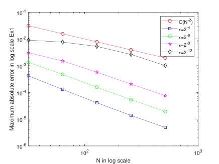
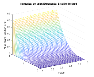
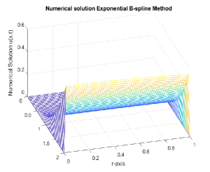
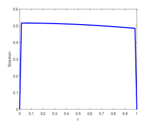
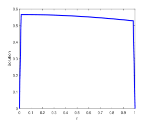
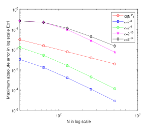
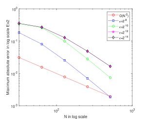
In order to validate the theoretical assumptions, an exponential B-spline collocation method on a Shishkin mesh is engaged on problems Example 12, Example 13 and Example 14. The maximum point-wise errors and the corresponding order of convergence is presented in Table 2, Table 4 and Table 6 for various values of $\epsilon$ and $\alpha =0.8$. As indicated by the tables, when $\epsilon \to 0$, the numerical examples’ results exhibit uniform convergence and almost second-order convergence in agreement with theoretical assumption. Additionally, the maximum point-wise error falls as the number of grid points rises. The maximum point-wise absolute errors for various values $\alpha$ and fixed $\epsilon =2^{-10}$ are provided in Table 3, Table 5 and Table 7. The results demonstrate that as $\alpha$ decreases, so does the maximum absolute error, providing that the fractional order model accurately depicts problems in the real world. The physical behavior of the system is displayed in Fig. 1(a) and (b) which provides numerical examples with twin layers at the end of spatial domain. The boundary layer behavior is confirmed by figures Fig. 2(a) and (b), which show a potential parabolic boundary layers at $r=0$ and $r=1$. The point-wise maximum absolute error on log-log scale is also displayed in Fig. 3 and Fig. 4. It exhibits when the number of grid points increases and $\epsilon \to 0$ the maximum absolute error decreases monotonically, showing a correlation with the theoretical results.

6. Conclusions

An exponential B-spline collocation technique is implemented to address the one-dimensional initial boundary value problem of singularly perturbed time fractional delay parabolic reaction-diffusion equations. Using the implicit Euler’s method, the time-fractional derivative is utilized by the Caputo fractional sense. An exponential B-spline collocation approach is conducted to handle the spatial domain on Shishkin mesh. The convergence analysis of the scheme is established and has an accurate of order $𝒪(N^{-2}{(\ln N)}^2)$. The findings from numerical examples verified an agreement of the method, which has twin layers at $r=0$ and $r=1$.

References

- [1] R.L. Bagley, P.J. Torvik, A theoretical basis for the application of fractional calculus to viscoelasticity, J. Rheol., 27 (1983) no. 3, pp. 201–210. https://doi.org/10.1122/1.549724
- [2] D.A. Benson, S.W. Wheatcraft and M.M. Meerschaert, Application of a fractional advection-dispersion equation, Water. Resour. Res., 36 (2000) no. 6, pp. 1403–1412. https://doi.org/10.1029/2000WR900031
- [3] A.D. Fitt, A.R.H. Goodwin, K.A. Ronaldson and W.A. Wakeham, A fractional differential equation for a MEMS viscometer used in the oil industry, J. Comput. Appl. Math., 229 (2009) no. 2, pp. 373–381. https://doi.org/10.1016/j.cam.2008.04.018
- [4] M. Oeser and S. Freitag, Modeling of materials with fading memory using neural networks, Int. J. Numer. Methods. Eng., 78 (2009) no. 7, pp. 843–862. https://doi.org/10.1002/nme.2518
- [5] A.A. Kilbas, H.M. Srivastava and J.J. Trujillo, Theory and applications of fractional differential equations, 204, Elsevier, 2006.
- [6] C. Jadhav, T. Dale and S. Dhondge, A Review on Applications of Fractional Differential Equations in Engineering Domain, MSEA, 71 (2022) no. 4, pp. 7147–7166. https://doi.org/10.17762/msea.v71i4.1331
- [7] R. Choudhary, S. Singh and D. Kumar, A second-order numerical scheme for the time-fractional partial differential equations with a time delay, Comput. Appl. Math., 41 (2022) no. 3, 114. https://doi.org/10.1007/s40314-022-01810-9
- [8] W.T. Aniley and G.F. Duressa, Nonstandard finite difference method for time-fractional singularly perturbed convection-diffusion problems with a delay in time, Results Appl. Math., 21 (2024), 100432. https://doi.org/10.1016/j.rinam.2024.100432
- [9] P. Pandey, S. Kumar, J.F. Gomez-Aguilar and D. Baleanu, An efficient technique for solving the space-time fractional reaction-diffusion equation in porous media, Chin. J. Phys., 68 (2020), pp. 483–492. https://doi.org/10.1016/j.cjph.2020.09.031
- [10] V. Gafiychuk, B. Datsko and V. Meleshko, Mathematical modeling of time fractional reaction-diffusion systems, J. Comput. Appl. Math., 220 (2008) no. 1-2, pp. 215–225. https://doi.org/10.1016/j.cam.2007.08.011
- [11] J. Zhang and X. Yang, A class of efficient difference method for time fractional reaction-diffusion equation, Comput. Appl. Math., 37 (2018) no. 4, pp. 4376–4396. https://doi.org/10.1007/s40314-018-0579-5
- [12] K. Van Bockstal, M.A. Zaky and A.S. Hendy, On the existence and uniqueness of solutions to a nonlinear variable order time-fractional reaction-diffusion equation with delay, Commun. Nonlinear Sci. Numer. Simul., 115 (2022), 106755. https://doi.org/10.1016/j.cnsns.2022.106755
- [13] T. Hamadneh, Z. Chebana, I. Abu Falahah, Y.A. Al-Khassawneh, A. Al-Husban, T.E. Oussaeif and A. Abbes, On finite-time blow-up problem for nonlinear fractional reaction-diffusion equation: analytical results and numerical simulations, Fractal Fract., 7 (2023) no. 8, 589. https://doi.org/10.3390/fractalfract7080589
- [14] N.T. Negero, A robust fitted numerical scheme for singularly perturbed parabolic reaction-diffusion problems with a general time delay, Results Phys., 51 (2023), 106724. https://doi.org/10.1016/j.rinp.2023.106724
- [15] A.R. Ansari, S.A. Bakr and G.I. Shishkin, A parameter-robust finite difference method for singularly perturbed delay parabolic partial differential equations, J. Comput. Appl. Math., 205 (2007) no. 1, pp. 552–566. https://doi.org/10.1016/j.cam.2006.05.032
- [16] J.J. Miller, E. O’riordan, and G.I. Shishkin, Fitted numerical methods for singular perturbation problems: error estimates in the maximum norm for linear problems in one and two dimensions, World scientific, 1996.
- [17]
- [18] R.N. Rao and P.P. Chakravarthy, A fitted Numerov method for singularly perturbed parabolic partial differential equation with a small negative shift arising in control theory, Numer. Math-Theory M.E., 7 (2014) no. 1, pp. 23–40. https://doi.org/10.1017/S1004897900000271
- [19] F.W. Gelu and G.F. Duressa, A uniformly convergent collocation method for singularly perturbed delay parabolic reaction-diffusion problem, Abstr. Appl. Anal., 2021 (2021), pp. 1–11. https://doi.org/10.1155/2021/8835595
- [20] E.A. Megiso, M.M. Woldaregay and T.G. Dinka, Fitted tension spline method for singularly perturbed time delay reaction diffusion problems, Math. Probl. Eng., 2022 (2022). https://doi.org/10.1155/2022/8669718
- [21] A.A. Tiruneh, G.A. Derese and D.M. Tefera, A nonstandard fitted operator method for singularly perturbed parabolic reaction-diffusion problems with a large time delay, Int. J. Math. Sci., 2022 (2022), pp. 1–11. https://doi.org/10.1155/2022/5625049
- [22] K. Khari and V. Kumar, Finite element analysis of the singularly perturbed parabolic reaction-diffusion problems with retarded argument, Numer. Methods Partial Differ. Equ., 38 (2022) no. 4, pp. 997–1014. https://doi.org/10.1002/num.22785
- [23] J. Howlader, P. Mishra and K.K. Sharma, An orthogonal spline collocation method for singularly perturbed parabolic reaction-diffusion problems with time delay, J. Appl. Math., Comput., 70 (2024) no. 2, pp. 1069–1101. https://doi.org/10.1007/s12190-024-01993-w
- [24] B.J. McCartin, Computation of exponential splines, SIAM J. Sci. Comput., 11 (1990) no. 2, pp. 242-–262. https://doi.org/10.1137/0911015
- [25] D. Radunovic, Multiresolution exponential B-splines and singularly perturbed boundary problem, Numer. Algor., 47 (2008), pp. 191–210. https://doi.org/10.1007/s11075-008-9171-1
- [26] O. Ersoy, and I. Dag, The exponential cubic B-spline algorithm for Korteweg-de Vries equation, Adv. Numer. Anal., 2015 (2015) no. 1, 367056. https://doi.org/10.1155/2015/367056
- [27] S.C.S. Rao and M. Kumar, Exponential B-spline collocation method for self-adjoint singularly perturbed boundary value problems, Appl. Numer. Math. 58 (2008) no. 10, pp. 1572–1581. https://doi.org/10.1016/j.apnum.2007.09.008
- [28] P.A. Selvi and N. Ramanujam, A parameter uniform difference scheme for singularly perturbed parabolic delay differential equation with Robin type boundary condition, Appl. Math. Comput., 296 (2017), pp. 101–115. https://doi.org/10.1016/j.amc.2016.10.027
- [29] C. Hall, On error bounds for spline interpolation, J. Approx. Theory, 1 (1968) no. 2, pp. 209–218. https://doi.org/10.1016/0021-9045(68)90025-7