Numerical Analysis and Stability of the Moore-Gibson-Thompson-Fourier Model

Ali Smouk^∗ and Atika Radid^†

(Date: October 2, 2024; accepted: November 2, 2024; published online: December 18, 2024.)

Abstract.

This work is concerned the Moore-Gibson-Thompson-Fourier Model. Our contribution will consist in studying the numerical stability of the Moore-Gibson-Thompson-Fourier system. First we introduce a finite element approximation after the discretization, then we prove that the associated discrete energy decreases and later we establish a priori error estimates. Finally, we obtain some numerical simulations.

Key words and phrases:

Moore-Gibson-Thompson-Fourier model, numerical stability, finite element method, numerical simulations

2005 Mathematics Subject Classification:

35L45,55, 65M60, 65N12, 93D23

^∗LMFA, Faculty of Sciences Aïn Chock, Hassan 2 University, Casablanca, Morocco, e-mail: smouk.ali.10@gmail.com.

^†LMFA, Faculty of Sciences Aïn Chock, Hassan 2 University, Casablanca, Morocco, e-mail: atikaradid@gmail.com.

1. Introduction

In this paper, we consider a Moore-Gibson-Thompson (MGT) equation

(1)

u_{ttt}+\alpha u_{tt}+\beta Au_{t}+\gamma Au=0,

which describes the evolution of the unknown function $u=u(x,t):\Omega\times[0,\infty)\rightarrow\mathbb{R}$ , where $\Omega\subset\mathbb{R}^{N}$ is a bounded domain with a sufficiently smooth boundary $\partial\Omega$ . The equation includes various parameters such as $\alpha,\beta,\gamma>0$ , which are fixed structural parameters.

Originally, for the Laplace-Dirichlet operator $A=-\Delta$ this equation was introduced to model wave propagation in viscous thermally relaxing fluids [14, 17], with its first appearance dating back to a paper by Stokes [15]. Over time, researchers have discovered that the MGT equation finds applications in a wide range of physical phenomena, including viscoelasticity and thermal conduction. Notably, it has been interpreted as a model for vibrations in a standard linear viscoelastic solid [9, 10].

In the particular case where $A=\Delta^{2}$ , with proper boundary conditions (see [12]), the MGT equation appears as a possible model for the vertical displacement in viscoelastic plates.

The mathematical analysis of the MGT equation has attracted significant attention, resulting in a vast literature with numerous studies and references available [4, 5, 11, 13, 2, 3, 16]. The main findings can be summarized as follows:

For any positive values of the parameters $\alpha,\beta,\gamma$ , the MGT equation generates a strongly continuous semigroup of solutions. However, the behavior of these solutions depends significantly on the constant $\nu$ , defined as follows:

\nu=\alpha\beta-\gamma.

For $A=\Delta^{2}$ the semigroup of MGT equation is analytic and exponentially stable the case of $\nu>0$ .

In present paper, we consider the MGT-Fourier system

(2)

\left\{\begin{array}[]{l}u_{ttt}+\alpha u_{tt}+\beta\Delta^{2}u_{t}+\gamma%\Delta^{2}u=-\eta\Delta\theta,\\\theta_{t}-\kappa\Delta\theta=\eta\Delta u_{tt}+\alpha\eta\Delta u_{t}\end{%array}\right.

where, the unknown function $u=u(x,t)$ represents the vibration of flexible structures and $\theta=\theta(x,t)$ the difference of temperature between the actual state and a reference temperature where $x\in\Omega,t\in(0,\infty)$ . The parameters $\alpha,\beta,\gamma$ and $\kappa$ are positive real numbers, $\eta\neq 0$ and $\Omega=[0,1]$ is a bounded domain. We assume the initial conditions

(3)

u(x,0)=u_{0},\quad u_{t}(x,0)=u_{1},\quad u_{tt}(x,0)=u_{2},\quad\theta(x,0)=%\theta_{0}

where $u_{0},u_{1},u_{2},\theta_{0}:\Omega\rightarrow\mathbb{R}$ are assigned initial data. The system is complemented with the boundary conditions

(4)

\displaystyle u(x,t)=\tfrac{\partial u}{\partial\nu}(x,t)=\theta(x,t)=0,\quad x%\in\partial\Omega

Now, we intoduce a new variable $z=u_{t}+\alpha u$ and using $\nu=\alpha\beta-\gamma$ . Consequently, the system $Math input error$ is equivalent to

(5)

\left\{\begin{array}[]{l}z_{tt}+\tfrac{\gamma}{\alpha}\Delta^{2}z+\tfrac{\nu}{%\alpha}\Delta^{2}u_{t}+\eta\Delta\theta=0,\\\theta_{t}-\kappa\Delta\theta-\eta\Delta z_{t}=0.\end{array}\right.

Associated to (2)–(4), we consider the energy functional

(6)		$\displaystyle E(t)$	$\displaystyle=\tfrac{1}{2}\left(\\|z_{t}\\|^{2}+\tfrac{\gamma}{\alpha}\\|\Delta z%\\|^{2}+\tfrac{\nu}{\alpha}\\|\Delta u_{t}\\|^{2}\right.+\left.\\|\theta\\|^{2}\right)$
		$\displaystyle=\tfrac{1}{2}\left(\\|u_{tt}+\alpha u_{t}\\|^{2}+\tfrac{\gamma}{%\alpha}\\|\Delta u_{t}+\alpha\Delta u\\|^{2}+\tfrac{\nu}{\alpha}\\|\Delta u_{t}\\|%^{2}\right.+\left.\\|\theta\\|^{2}\right)$

Theorem 1 ([8]).

The semigroup associate to $Math input error$ is analytic and exponentially stable for $\nu>0$ .

As a results from [8] the energy $Math input error$ decays exponentially for $\nu>0$ , that is, there exist two positive constants $\epsilon_{1},\epsilon_{2}$ such that

E(t)\leq\epsilon_{1}e^{-\epsilon_{2}t};\quad\text{for all }t\geq 0.

and satisfies

(7)

E^{\prime}(t)=-\nu\|\Delta u_{t}\|^{2}-\kappa\|\nabla\theta\|^{2}\leq 0,

For further details, refer to [8].

2. Numerical approximation

In this section, we propose a finite element approximation to system $Math input error$ with boundary conditions $Math input error$ and initial conditions $Math input error$ .

We introduce and study finite elements in space and an implicit Euler type scheme based on finite differences in time. We prove that the discrete energy decays.

Introducing new variables $y=z_{t}$ , $v=u_{t}$ , $\Phi=-\Delta z$ and $\Psi=-\Delta v$ ; we rewrite system $Math input error$

(8)

\left\{\begin{aligned} &y_{t}-\tfrac{\gamma}{\alpha}\Delta\Phi-\tfrac{\nu}{%\alpha}\Delta\Psi+\eta\Delta\theta=0,\\&\theta_{t}-\kappa\Delta\theta-\eta\Delta y=0\\&-\Delta z=\Phi\\&-\Delta v=\Psi.\end{aligned}\right.

In order to obtain the weak form associated with system $Math input error$ , we multiply the equations by test functions $\chi,\xi,\omega,\zeta\in H_{0}^{1}(0,1)$ and integrate by parts.

(9)

\left\{\begin{aligned} &\left(y_{t},\chi\right)+\tfrac{\gamma}{\alpha}\left(%\nabla\Phi,\nabla\chi\right)+\tfrac{\nu}{\alpha}\left(\nabla\Psi,\nabla\chi%\right)-\eta\left(\nabla\theta,\nabla\chi\right)=0,\\&\left(\theta_{t},\xi\right)+\kappa\left(\nabla\theta,\nabla\xi\right)+\eta%\left(\nabla y,\nabla\xi\right)=0\\&\left(\nabla z,\nabla\omega\right)-\left(\Phi,\omega\right)=0\\&\left(\nabla v,\nabla\zeta\right)-\left(\Psi,\zeta\right)=0.\end{aligned}\right.

For our purposes, we considered $J$ a nonnegative integer and $h=\tfrac{1}{J}\$ a subdivision of the interval $(0,1)$ given by $0=x_{0}<x_{1}<\ldots<x_{J-1}<x_{J}=1$ , such that $x_{j}=jh$ , for all $j=0,\ldots,J$ . We take

(10)		$\displaystyle S^{h}=\left\{\right.g\in H^{1}\left(0,1\right)\left\|\right.\ g%\in C\left(\left[0,1\right]\right),$	$\displaystyle g\left\|\right._{(x_{j},x_{j+1})}\ \text{is a linearpolynomial, with }$
(10)			$\displaystyle\left.j=0,\ldots,J-1\right\}$

and

S_{0}^{h}=\left\{g\in S^{h}\left|\ g(0)=g(1)=0\right.\right\}.

For a given final time $T$ and a positive integer $N$ , let $\triangle t=T/N$ be the time step and $t_{n}=n\Delta t,\ n=0,\ldots,N.$

The finite element method for $Math input error$ using the backward Euler scheme is to find $y_{h}^{n},\ \theta_{h}^{n},\ \Phi_{h}^{n},\ \Psi_{h}^{n}\in S_{0}^{h}$ such that, for $n=1,\ldots,N$ and for all $\chi_{h},\ \xi_{h},\ \omega_{h},\ \zeta_{h}\in S_{0}^{h}$

(11)

\displaystyle\left\{\begin{aligned} &\tfrac{1}{\Delta t}\left(y_{h}^{n}-y_{h}^%{n-1},\chi_{h}\right)+\tfrac{\gamma}{\alpha}\left(\nabla\Phi_{h}^{n},\nabla%\chi_{h}\right)+\tfrac{\nu}{\alpha}\left(\nabla\Psi_{h}^{n},\nabla\chi_{h}%\right)-\eta\left(\nabla\theta_{h}^{n},\nabla\chi_{h}\right)=0,\\&\tfrac{1}{\Delta t}\left(\theta_{h}^{n}-\theta_{h}^{n-1},\xi_{h}\right)+%\kappa\left(\nabla\theta_{h}^{n},\nabla\xi_{h}\right)+\eta\left(\nabla y_{h}^{%n},\nabla\xi_{h}\right)=0,\\&\left(\nabla z_{h}^{n},\nabla\omega_{h}\right)-\left(\Phi_{h}^{n},\omega_{h}%\right)=0\\&\left(\nabla v_{h}^{n},\nabla\zeta_{h}\right)-\left(\Psi_{h}^{n},\zeta_{h}%\right)=0.\end{aligned}\right.

where

(12)

v_{h}^{n}=\tfrac{u_{h}^{n}-u_{h}^{n-1}}{\triangle t},\ z_{h}^{n}=v_{h}^{n}+%\alpha u_{h}^{n},\ \text{and}\ y_{h}^{n}=\tfrac{z_{h}^{n}-z_{h}^{n-1}}{%\triangle t},

are approximations to $u_{t}\left(t_{n}\right),\ v\left(t_{n}\right)+\alpha u\left(t_{n}\right),\ z_{%t}\left(t_{n}\right)$ respectively.

By leveraging the properties of inner products and norms, we derive the following identity, which will be frequently used:

(13)

\left(a-b,a\right)=\tfrac{1}{2}\left(\left\|a-b\right\|^{2}+\left\|a\right\|^{%2}-\left\|b\right\|^{2}\right).

The next result is a discrete version of the energy decay property satisfied by the solution of system $Math input error$ .

We introduce the following discrete energy,

(14)

\displaystyle\mathcal{E}_{h}^{n}

\displaystyle=\tfrac{1}{2}\left(\|y_{h}^{n}\|^{2}+\tfrac{\gamma}{\alpha}\|\Phi%_{h}^{n}\|^{2}+\tfrac{\nu}{\alpha}\|\Psi_{h}^{n}\|^{2}+\|\theta_{h}^{n}\|^{2}%\right).

Theorem 2.

The discrete energy decay to zero, that is,

(15)

\tfrac{\mathcal{E}_{h}^{n}-\mathcal{E}_{h}^{n-1}}{\triangle t}\leq 0,

holds for $n=1,2,\ldots,N$ .

Proof.

Taking $\chi_{h}=y_{h}^{n}$ and $\xi_{h}=\theta_{h}^{n}$ in $Math input error$ .

(16)

\left\{\begin{aligned} &\tfrac{1}{\Delta t}\left(y_{h}^{n}-y_{h}^{n-1},y_{h}^{%n}\right)+\tfrac{\gamma}{\alpha}\left(\nabla\Phi_{h}^{n},\nabla y_{h}^{n}%\right)+\tfrac{\nu}{\alpha}\left(\nabla\Psi_{h}^{n},\nabla y_{h}^{n}\right)-%\eta\left(\nabla\theta_{h}^{n},\nabla y_{h}^{n}\right)=0,\\&\tfrac{1}{\Delta t}\left(\theta_{h}^{n}-\theta_{h}^{n-1},\theta_{h}^{n}\right%)+\kappa\left(\nabla\theta_{h}^{n},\nabla\theta_{h}^{n}\right)+\eta\left(%\nabla y_{h}^{n},\nabla\theta_{h}^{n}\right)=0.\end{aligned}\right.

Summing equations of system $Math input error$ , we have

(17)		$\displaystyle\tfrac{1}{\Delta t}\left(y_{h}^{n}-y_{h}^{n-1},y_{h}^{n}\right)+%\tfrac{\gamma}{\alpha}\left(\nabla\Phi_{h}^{n},\nabla y_{h}^{n}\right)+\tfrac{%\nu}{\alpha}\left(\nabla\Psi_{h}^{n},\nabla y_{h}^{n}\right)$	$\displaystyle+\tfrac{1}{\Delta t}\left(\theta_{h}^{n}-\theta_{h}^{n-1},\theta_%{h}^{n}\right)+$
(17)			$\displaystyle+\kappa\left(\nabla\theta_{h}^{n},\nabla\theta_{h}^{n}\right)=0.$

Recalling $Math input error$ and $Math input error$ , we have

(18)

\tfrac{1}{\Delta t}\left(y_{h}^{n}-y_{h}^{n-1},y_{h}^{n}\right)=\tfrac{1}{2%\Delta t}\left(\left\|y_{h}^{n}-y_{h}^{n-1}\right\|^{2}+\left\|y_{h}^{n}\right%\|^{2}-\left\|y_{h}^{n-1}\right\|^{2}\right).

Next,

(19)	$\displaystyle\tfrac{\gamma}{\alpha}\left(\nabla\Phi_{h}^{n},\nabla y_{h}^{n}\right)$	$\displaystyle=-\tfrac{\gamma}{\alpha}\left(\Phi_{h}^{n},\Delta y_{h}^{n}\right)=$
	$\displaystyle=-\tfrac{\gamma}{\alpha}\left(\Phi_{h}^{n},\tfrac{\Delta z_{h}^{n%}-\Delta z_{h}^{n-1}}{\triangle t}\right)$
	$\displaystyle=\tfrac{\gamma}{\alpha}\left(\Phi_{h}^{n},\tfrac{\Phi_{h}^{n}-%\Phi_{h}^{n-1}}{\triangle t}\right)$
	$\displaystyle=\tfrac{\gamma}{2\alpha\Delta t}\left(\left\\|\Phi_{h}^{n}-\Phi_{h%}^{n-1}\right\\|^{2}+\left\\|\Phi_{h}^{n}\right\\|^{2}-\left\\|\Phi_{h}^{n-1}%\right\\|^{2}\right).$

Similarly,

(20)	$\displaystyle\tfrac{\nu}{\alpha}\left(\nabla\Psi_{h}^{n},\nabla y_{h}^{n}\right)$	$\displaystyle=-\tfrac{\nu}{\alpha}\left(\Psi_{h}^{n},\Delta y_{h}^{n}\right)$
	$\displaystyle=-\tfrac{\nu}{\alpha}\left(\Psi_{h}^{n},\tfrac{\Delta z_{h}^{n}-%\Delta z_{h}^{n-1}}{\triangle t}\right)$
	$\displaystyle=-\tfrac{\nu}{\alpha}\left(\Psi_{h}^{n},\tfrac{\Delta(v_{h}^{n}+%\alpha u_{h}^{n})-\Delta(v_{h}^{n-1}+\alpha u_{h}^{n-1})}{\triangle t}\right)$
	$\displaystyle=-\tfrac{\nu}{\alpha}\left(\Psi_{h}^{n},\tfrac{\Delta v_{h}^{n}-%\Delta v_{h}^{n-1}}{\triangle t}\right)-\nu\left(\Psi_{h}^{n},\tfrac{\Delta u_%{h}^{n}-\Delta u_{h}^{n-1}}{\triangle t}\right)$
	$\displaystyle=\tfrac{\nu}{\alpha}\left(\Psi_{h}^{n},\tfrac{\Psi_{h}^{n}-\Psi_{%h}^{n-1}}{\triangle t}\right)+\nu\left(\Psi_{h}^{n},\Psi_{h}^{n}\right)$
	$\displaystyle=\tfrac{\nu}{2\alpha\Delta t}\left(\left\\|\Psi_{h}^{n}-\Psi_{h}^{%n-1}\right\\|^{2}+\left\\|\Psi_{h}^{n}\right\\|^{2}-\left\\|\Psi_{h}^{n-1}\right\\|%^{2}\right)+\nu\left\\|\Psi_{h}^{n}\right\\|^{2}.$

Also,

(21)

\tfrac{1}{\Delta t}\left(\theta_{h}^{n}-\theta_{h}^{n-1},\theta_{h}^{n}\right)%=\tfrac{1}{2\Delta t}\left(\left\|\theta_{h}^{n}-\theta_{h}^{n-1}\right\|^{2}+%\left\|\theta_{h}^{n}\right\|^{2}-\left\|\theta_{h}^{n-1}\right\|^{2}\right).

Thus,

	$\displaystyle\tfrac{1}{2\Delta t}\left(\left\\|y_{h}^{n}-y_{h}^{n-1}\right\\|^{2%}+\left\\|y_{h}^{n}\right\\|^{2}-\left\\|y_{h}^{n-1}\right\\|^{2}\right)+$
(22)		$\displaystyle\quad+\tfrac{\gamma}{2\alpha\Delta t}\left(\left\\|\Phi_{h}^{n}-%\Phi_{h}^{n-1}\right\\|^{2}+\left\\|\Phi_{h}^{n}\right\\|^{2}-\left\\|\Phi_{h}^{n-%1}\right\\|^{2}\right)$
	$\displaystyle\quad+\tfrac{\nu}{2\alpha\Delta t}\left(\left\\|\Psi_{h}^{n}-\Psi_%{h}^{n-1}\right\\|^{2}+\left\\|\Psi_{h}^{n}\right\\|^{2}-\left\\|\Psi_{h}^{n-1}%\right\\|^{2}\right)+\nu\left\\|\Psi_{h}^{n}\right\\|^{2}$
	$\displaystyle\quad+\tfrac{1}{2\Delta t}\left(\left\\|\theta_{h}^{n}-\theta_{h}^%{n-1}\right\\|^{2}+\left\\|\theta_{h}^{n}\right\\|^{2}-\left\\|\theta_{h}^{n-1}%\right\\|^{2}\right)+\kappa\left\\|\nabla\theta_{h}^{n}\right\\|^{2}=0.$

We deduce that

	$\displaystyle 0$	$\displaystyle=\tfrac{1}{2\Delta t}\left(\left\\|y_{h}^{n}-y_{h}^{n-1}\right\\|^{%2}+\left\\|y_{h}^{n}\right\\|^{2}-\left\\|y_{h}^{n-1}\right\\|^{2}\right)$
		$\displaystyle\quad+\tfrac{\gamma}{2\alpha\Delta t}\left(\left\\|\Phi_{h}^{n}-%\Phi_{h}^{n-1}\right\\|^{2}+\left\\|\Phi_{h}^{n}\right\\|^{2}-\left\\|\Phi_{h}^{n-%1}\right\\|^{2}\right)$
(23)			$\displaystyle\quad+\tfrac{\nu}{2\alpha\Delta t}\left(\left\\|\Psi_{h}^{n}-\Psi_%{h}^{n-1}\right\\|^{2}+\left\\|\Psi_{h}^{n}\right\\|^{2}-\left\\|\Psi_{h}^{n-1}%\right\\|^{2}\right)+\nu\left\\|\Psi_{h}^{n}\right\\|^{2}$
		$\displaystyle\quad+\tfrac{1}{2\Delta t}\left(\left\\|\theta_{h}^{n}-\theta_{h}^%{n-1}\right\\|^{2}+\left\\|\theta_{h}^{n}\right\\|^{2}-\left\\|\theta_{h}^{n-1}%\right\\|^{2}\right)+\kappa\left\\|\nabla\theta_{h}^{n}\right\\|^{2}$
		$\displaystyle\geq\tfrac{\mathcal{E}_{h}^{n}-\mathcal{E}_{h}^{n-1}}{\triangle t}.$

Which implies $\tfrac{\mathcal{E}_{h}^{n}-\mathcal{E}_{h}^{n-1}}{\triangle t}\leq 0$ and this completes the proof. ∎

Now, we prove a main error estimates result.

Theorem 3.

There exists a positive constant $C$ , independent of the discretization parameters $h$ and $\Delta t$ such that for all $\left\{\chi_{h}^{i},\xi_{h}^{i}\ \right\}^{i=0}_{N}\subset S_{0}^{h}$ ,

(24)		$\displaystyle\max_{0\leq n\leq N}\left\{\left\\|y^{n}-y_{h}^{n}\right\\|^{2}+%\left\\|\Phi^{n}-\Phi_{h}^{n}\right\\|^{2}+\left\\|\Psi^{n}-\Psi_{h}^{n}\right\\|^%{2}+\left\\|\theta^{n}-\theta_{h}^{n}\right\\|^{2}\right\}\leq$
	$\displaystyle\leq C\Delta t\sum_{i=1}^{N}\left(\left\\|y_{t}^{i}-\delta y^{i}%\right\\|^{2}+\left\\|\Phi_{t}^{i}-\delta\Phi^{i}\right\\|^{2}+\left\\|\Psi_{t}^{i%}-\delta\Psi^{i}\right\\|^{2}+\left\\|\theta_{t}^{i}-\delta\theta^{i}\right\\|^{2%}\right.$
	$\displaystyle\quad\left.+\left\\|\nabla y^{i}-\nabla\chi_{h}^{i}\right\\|^{2}+%\left\\|\nabla\theta^{i}-\nabla\xi_{h}^{i}\right\\|^{2}\right)+C\max_{0\leq n%\leq N}\left\{\left\\|y^{n}-\chi_{h}^{n}\right\\|^{2}+\left\\|\theta^{n}-\xi_{h}^%{n}\right\\|^{2}\right\}$
	$\displaystyle\quad+\tfrac{C}{\Delta t}\sum_{i=1}^{N-1}\left(\left\\|y^{i}-\chi_%{h}^{i}-\left(y^{i+1}-\chi_{h}^{i+1}\right)\right\\|^{2}+\left\\|\theta^{i}-\xi_%{h}^{i}-\left(\theta^{i+1}-\xi_{h}^{i+1}\right)\right\\|^{2}\right)$
	$\displaystyle\quad+C\left(\left\\|y^{0}-y_{h}^{0}\right\\|^{2}+\left\\|\Phi^{0}-%\Phi_{h}^{0}\right\\|^{2}+\left\\|\Psi^{0}-\Psi_{h}^{0}\right\\|^{2}+\left\\|%\theta^{0}-\theta_{h}^{0}\right\\|^{2}\right),$

where $\delta f^{i}=\left(f^{i}-f^{i-1}\right)/\Delta t$ .

Proof.

First, we subtract the first variational equation in $Math input error$ at time $t=t_{n}$ for a test function $\chi=\chi_{h}\in S_{0}^{h}\subset H_{0}^{1}\left(0,1\right)$ and the first discrete variational equation in $Math input error$ to obtain

(25)			$\displaystyle\left(y_{t}^{n}-\delta y_{h}^{n},\chi_{h}\right)+\tfrac{\gamma}{%\alpha}\left(\nabla\Phi^{n}-\nabla\Phi_{h}^{n},\nabla\chi_{h}\right)+\tfrac{%\nu}{\alpha}\left(\nabla\Psi^{n}-\nabla\Psi_{h}^{n},\nabla\chi_{h}\right)-$
		$\displaystyle-\eta\left(\nabla\theta^{n}-\nabla\theta_{h}^{n},\nabla\chi_{h}%\right)=0,\ \text{for all }\chi_{h}\in S_{0}^{h}$

and so, we have

(26)		$\displaystyle\left(y_{t}^{n}\!-\!\delta y_{h}^{n},y^{n}\!-\!y_{h}^{n}\right)\!%+\!\tfrac{\gamma}{\alpha}\left(\nabla\Phi^{n}\!-\!\nabla\Phi_{h}^{n},\nabla(y^%{n}\!-\!y_{h}^{n})\right)\!+\!\tfrac{\nu}{\alpha}\left(\nabla\Psi^{n}\!-\!%\nabla\Psi_{h}^{n},\nabla(y^{n}-y_{h}^{n})\right)$
	$\displaystyle\quad-\eta\left(\nabla\theta^{n}-\nabla\theta_{h}^{n},\nabla(y^{n%}-y_{h}^{n})\right)$
	$\displaystyle=\left(y_{t}^{n}\!-\!\delta y_{h}^{n},y^{n}\!-\!\chi_{h}\right)\!%+\!\tfrac{\gamma}{\alpha}\left(\nabla\Phi^{n}\!-\!\nabla\Phi_{h}^{n},\nabla(y^%{n}\!-\!\chi_{h})\right)\!+\!\tfrac{\nu}{\alpha}\left(\nabla\Psi^{n}\!-\!%\nabla\Psi_{h}^{n},\nabla(y^{n}\!-\!\chi_{h})\right)$
	$\displaystyle\quad-\eta\left(\nabla\theta^{n}-\nabla\theta_{h}^{n},\nabla(y^{n%}-\chi_{h})\right),\ \text{for all }\chi_{h}\in S_{0}^{h}$

Taking into account that

	$\displaystyle\left(y_{t}^{n}-\delta y_{h}^{n},y^{n}-y_{h}^{n}\right)$	$\displaystyle\!=\!\left(y_{t}^{n}\!\!-\!\!\delta y^{n},y^{n}\!-\!y_{h}^{n}%\right)\!+\!\left(\delta y^{n}\!-\!\delta y_{h}^{n},y^{n}\!-\!y_{h}^{n}\right)%\!=\!\left(y_{t}^{n}\!-\!\delta y^{n},y^{n}\!-\!y_{h}^{n}\right)$
		$\displaystyle\quad\!+\!\tfrac{1}{2\Delta t}\left(\left\\|y^{n}\!\!-\!\!y_{h}^{n%}\!\!-\!\!(y^{n-1}\!\!-\!\!y_{h}^{n-1})\right\\|^{2}\!\!+\!\!\left\\|y^{n}\!\!-%\!\!y_{h}^{n}\right\\|^{2}\!\!-\!\!\left\\|y^{n-1}\!\!-\!\!y_{h}^{n-1}\right\\|^{%2}\right)$

By the positivity of the terms $\left\|y^{n}-y_{h}^{n}-(y^{n-1}-y_{h}^{n-1})\right\|^{2}$ , we get the following inequality

(27)	$\displaystyle\left(y_{t}^{n}\!-\!\delta y_{h}^{n},y^{n}\!-\!y_{h}^{n}\right)$	$\displaystyle\!\geq\!\left(y_{t}^{n}\!-\!\delta y^{n},y^{n}\!\!-\!\!y_{h}^{n}%\right)\!\!+\!\!\tfrac{1}{2\Delta t}\left(\left\\|y^{n}\!\!-\!\!y_{h}^{n}\right%\\|^{2}\!\!-\!\!\left\\|y^{n-1}\!-\!y_{h}^{n-1}\right\\|^{2}\right),$
	$\displaystyle\left(\nabla\Phi^{n}-\nabla\Phi_{h}^{n},\nabla(y^{n}-y_{h}^{n})\right)$	$\displaystyle=\left(\Phi_{t}^{n}-\delta\Phi_{h}^{n},\Phi^{n}-\Phi_{h}^{n}\right)$
		$\displaystyle=\left(\Phi_{t}^{n}-\delta\Phi^{n},\Phi^{n}-\Phi_{h}^{n}\right)+%\left(\delta\Phi^{n}-\delta\Phi_{h}^{n},\Phi^{n}-\Phi_{h}^{n}\right)$
		$\displaystyle\geq\left(\Phi_{t}^{n}-\delta\Phi^{n},\Phi^{n}-\Phi_{h}^{n}\right)$
		$\displaystyle\quad+\tfrac{1}{2\Delta t}\left(\left\\|\Phi^{n}-\Phi_{h}^{n})%\right\\|^{2}-\left\\|\Phi^{n-1}-\Phi_{h}^{n-1}\right\\|^{2}\right),$
	$\displaystyle\left(\nabla\Psi^{n}-\nabla\Psi_{h}^{n},\nabla(y^{n}-y_{h}^{n})\right)$	$\displaystyle=\left(\Psi^{n}-\Psi_{h}^{n},\Phi_{t}^{n}-\delta\Phi_{h}^{n}\right)$
		$\displaystyle=\left(\Psi^{n}-\Psi_{h}^{n},(\Psi_{t}^{n}+\alpha\Psi^{n})-(%\delta\Psi_{h}^{n}+\alpha\Psi_{h}^{n})\right)$
		$\displaystyle=\left(\Psi^{n}-\Psi_{h}^{n},\Psi_{t}^{n}-\delta\Psi_{h}^{n}%\right)+\alpha\left(\Psi^{n}-\Psi_{h}^{n},\Psi^{n}-\Psi_{h}^{n}\right)$
		$\displaystyle=\left(\Psi_{t}^{n}-\delta\Psi_{h}^{n},\Psi^{n}-\Psi_{h}^{n}%\right)+\alpha\left\\|\Psi^{n}-\Psi_{h}^{n}\right\\|^{2}$
		$\displaystyle\geq\left(\Psi_{t}^{n}-\delta\Psi^{n},\Psi^{n}-\Psi_{h}^{n}\right%)+\alpha\left\\|\Psi^{n}-\Psi_{h}^{n})\right\\|^{2}$
		$\displaystyle\quad+\tfrac{1}{2\Delta t}\left(\left\\|\Psi^{n}-\Psi_{h}^{n})%\right\\|^{2}-\left\\|\Psi^{n-1}-\Psi_{h}^{n-1}\right\\|^{2}\right).$

Second, we subtract the second variational equation in $Math input error$ at time $t=t_{n}$ for a test function $\xi=\xi_{h}\in S_{0}^{h}\subset H_{0}^{1}\left(0,1\right)$ and the second discrete variational equation in $Math input error$ to obtain

(28)

\displaystyle\left(\theta_{t}^{n}-\delta\theta_{h}^{n},\xi_{h}\right)+\kappa%\left(\nabla\theta^{n}-\nabla\theta_{h}^{n},\nabla\xi_{h}\right)+\eta\left(%\nabla y^{n}-\nabla y_{h}^{n},\nabla\xi_{h}\right)=0,

and so, we have

(29)			$\displaystyle\left(\theta_{t}^{n}-\delta\theta_{h}^{n},\theta^{n}-\theta_{h}^{%n}\right)+\kappa\left(\nabla\theta^{n}-\nabla\theta_{h}^{n},\nabla(\theta^{n}-%\theta_{h}^{n})\right)+\eta\left(\nabla y^{n}-\nabla y_{h}^{n},\nabla(\theta^{%n}-\theta_{h}^{n})\right)$
		$\displaystyle=\left(\theta_{t}^{n}-\delta\theta_{h}^{n},\theta^{n}-\xi_{h}%\right)\!+\!\kappa\left(\nabla\theta^{n}-\nabla\theta_{h}^{n},\nabla(\theta^{n%}-\xi_{h})\right)\!+\!\eta\left(\nabla y^{n}\!-\!\nabla y_{h}^{n},\nabla(%\theta^{n}-\xi_{h})\right).$

Taking into account that

(30)		$\displaystyle\left(\theta_{t}^{n}-\delta\theta_{h}^{n},\theta^{n}-y_{h}^{n}\right)$	$\displaystyle=\left(\theta_{t}^{n}-\delta\theta^{n},\theta^{n}-\theta_{h}^{n}%\right)+\left(\delta\theta^{n}-\delta\theta_{h}^{n},\theta^{n}-\theta_{h}^{n}\right)$
(30)			$\displaystyle\geq\left(\theta_{t}^{n}-\delta\theta^{n},\theta^{n}-\theta_{h}^{%n}\right)\!+\!\tfrac{1}{2\Delta t}\left(\left\\|\theta^{n}-\theta_{h}^{n}\right%\\|^{2}\!-\!\left\\|\theta^{n-1}-\theta_{h}^{n-1}\right\\|^{2}\right).$

From (26)–(27) and using several times Young’s inequality $Math input error$

(31)

ab\leq\varepsilon a^{2}+\tfrac{1}{4\varepsilon}b^{2},\quad a,b\in\mathbb{R},\,%\varepsilon\in\mathbb{R^{+*}}.

		$\displaystyle\left(y_{t}^{n}\!-\!\delta y^{n},y^{n}\!-\!y_{h}^{n}\right)\!+\!%\tfrac{1}{2\Delta t}\left(\left\\|y^{n}\!-\!y_{h}^{n}\right\\|^{2}\!-\!\left\\|y^%{n-1}\!-\!y_{h}^{n-1}\right\\|^{2}\right)\!+\!\left(\Phi_{t}^{n}-\delta\Phi^{n}%,\Phi^{n}-\Phi_{h}^{n}\right)+$
		$\displaystyle\quad\!+\!\tfrac{1}{2\Delta t}\left(\left\\|\Phi^{n}\!-\!\Phi_{h}^%{n})\right\\|^{2}\!-\!\left\\|\Phi^{n-1}\!-\!\Phi_{h}^{n-1}\right\\|^{2}\right)\!%\!+\!\!\left(\Psi_{t}^{n}\!-\!\delta\Psi^{n},\Psi^{n}\!-\!\Psi_{h}^{n}\right)+%\alpha\left\\|\Psi^{n}\!-\Psi_{h}^{n})\right\\|^{2}$
		$\displaystyle\quad\!+\!\tfrac{1}{2\Delta t}\left(\left\\|\Psi^{n}-\Psi_{h}^{n})%\right\\|^{2}-\left\\|\Psi^{n-1}-\Psi_{h}^{n-1}\right\\|^{2}\right)-\eta\left(%\nabla\theta^{n}-\nabla\theta_{h}^{n},\nabla(y^{n}-y_{h}^{n})\right)\leq$
		$\displaystyle\leq\left(y_{t}^{n}\!-\!\delta y_{h}^{n},y^{n}\!-\!y_{h}^{n}%\right)\!+\!\tfrac{\gamma}{\alpha}\left(\nabla\Phi^{n}\!-\!\nabla\Phi_{h}^{n},%\nabla(y^{n}-y_{h}^{n})\right)\!+\!\tfrac{\nu}{\alpha}\left(\nabla\Psi^{n}\!-%\!\nabla\Psi_{h}^{n},\nabla(y^{n}\!-\!y_{h}^{n})\right)$
		$\displaystyle\quad-\eta\left(\nabla\theta^{n}-\nabla\theta_{h}^{n},\nabla(y^{n%}-y_{h}^{n})\right)$
		$\displaystyle\!=\!\left(y_{t}^{n}\!\!-\!\!\delta y_{h}^{n},y^{n}-\chi_{h}%\right)\!+\!\tfrac{\gamma}{\alpha}\left(\nabla\Phi^{n}\!-\!\nabla\Phi_{h}^{n},%\nabla(y^{n}\!-\!\chi_{h})\right)\!+\!\tfrac{\nu}{\alpha}\left(\nabla\Psi^{n}%\!-\!\nabla\Psi_{h}^{n},\nabla(y^{n}\!-\!\chi_{h})\right)$
		$\displaystyle\quad-\eta\left(\nabla\theta^{n}-\nabla\theta_{h}^{n},\nabla(y^{n%}-\chi_{h})\right),\ \text{for all }\chi_{h}\in S_{0}^{h}.$

Next,

		$\displaystyle\tfrac{1}{2\Delta t}\left(\left\\|y^{n}-y_{h}^{n}\right\\|^{2}-%\left\\|y^{n-1}-y_{h}^{n-1}\right\\|^{2}\right)+\tfrac{1}{2\Delta t}\left(\left%\\|\Phi^{n}-\Phi_{h}^{n})\right\\|^{2}-\left\\|\Phi^{n-1}-\Phi_{h}^{n-1}\right\\|^%{2}\right)$
		$\displaystyle\quad\!\!+\!\!\alpha\left\\|\Psi^{n}\-\Psi_{h}^{n})\right\\|^{2}\!%\!+\!\!\tfrac{1}{2\Delta t}\left(\left\\|\Psi^{n}\!\!-\!\!\Psi_{h}^{n})\right\\|%^{2}\!\!-\!\!\left\\|\Psi^{n-1}\!\!-\!\!\Psi_{h}^{n-1}\right\\|^{2}\right)\!\!-%\!\!\eta\left(\nabla\theta^{n}\!-\!\nabla\theta_{h}^{n},\nabla(y^{n}\!-\!y_{h}%^{n})\right)$
		$\displaystyle\leq\left(y_{t}^{n}\!-\!\delta y_{h}^{n},y^{n}\!-\!\chi_{h}\right%)\!\!+\!\!\tfrac{\gamma}{\alpha}\left(\nabla\Phi^{n}\!-\!\nabla\Phi_{h}^{n},%\nabla(y^{n}-\chi_{h})\right)\!\!+\!\!\tfrac{\nu}{\alpha}\left(\nabla\Psi^{n}-%\nabla\Psi_{h}^{n},\nabla(y^{n}\!\!-\!\!\chi_{h})\right)$
		$\displaystyle\quad-\eta\left(\nabla\theta^{n}-\nabla\theta_{h}^{n},\nabla(y^{n%}-\chi_{h})\right)-\left(y_{t}^{n}-\delta y^{n},y^{n}-y_{h}^{n}\right)-\left(%\Phi_{t}^{n}-\delta\Phi^{n},\Phi^{n}-\Phi_{h}^{n}\right)$
		$\displaystyle\quad-\left(\Psi_{t}^{n}-\delta\Psi^{n},\Psi^{n}-\Psi_{h}^{n}%\right),\ \text{for all }\chi_{h}\in S_{0}^{h}.$

It follows that

(32)		$\displaystyle\tfrac{1}{2\Delta t}\left(\left\\|y^{n}-y_{h}^{n}\right\\|^{2}-%\left\\|y^{n-1}-y_{h}^{n-1}\right\\|^{2}\right)+\tfrac{\gamma}{2\alpha\Delta t}%\left(\left\\|\Phi^{n}-\Phi_{h}^{n})\right\\|^{2}-\left\\|\Phi^{n-1}-\Phi_{h}^{n-%1}\right\\|^{2}\right)$
	$\displaystyle\quad\!\!+\!\!\tfrac{\nu}{2\alpha\Delta t}\left(\left\\|\Psi^{n}\!%\!-\!\!\Psi_{h}^{n}\right\\|^{2}\!\!-\!\!\left\\|\Psi^{n-1}\!\!-\!\!\Psi_{h}^{n-%1}\right\\|^{2}\right)\!\!+\!\!\nu\left\\|\Psi^{n}\!\!-\!\!\Psi_{h}^{n}\right\\|^%{2}\!-\!\eta\left(\nabla\theta^{n}\!-\!\nabla\theta_{h}^{n},\nabla y^{n}\!\!-%\!\!\nabla y_{h}^{n}\right)$
	$\displaystyle\leq C\left(\left\\|y_{t}^{n}-\delta y^{n}\right\\|^{2}+\left\\|y^{n%}-y_{h}^{n}\right\\|^{2}+\left\\|\Phi_{t}^{n}-\delta\Phi^{n}\right\\|^{2}+\left\\|%\Phi^{n}-\Phi_{h}^{n})\right\\|^{2}\right.+\left\\|\Psi_{t}^{n}-\delta\Psi^{n}%\right\\|^{2}$
	$\displaystyle\quad\!+\!\left\\|\Psi^{n}\!-\!\Psi_{h}^{n})\right\\|^{2}\!+\!\left%\\|\nabla\theta^{n}\!-\!\nabla\theta_{h}^{n}\right\\|^{2}\!+\!\left\\|y^{n}\!-\!%\chi_{h}\right\\|^{2}+\left\\|\nabla y^{n}-\nabla\chi_{h}\right\\|^{2}\!+\!\left%\\|\Delta y^{n}-\Delta\chi_{h}\right\\|^{2}\left.\right)$
	$\displaystyle\quad+\left(\delta y^{n}-\delta y_{h}^{n},y^{n}-\chi_{h}\right),%\ \text{for all }\chi_{h}\in S_{0}^{h}.$

Proceeding with a similar approach for equations (29)-(30), we obtain the following estimates, for all $\xi_{h}\in S_{0}^{h}$ ,

(33)		$\displaystyle\tfrac{1}{2\Delta t}\left(\left\\|\theta^{n}\!-\!\theta_{h}^{n}%\right\\|^{2}\!-\!\left\\|\theta^{n-1}\!-\!\theta_{h}^{n-1}\right\\|^{2}\right)\!%+\!\kappa\left\\|\nabla\theta^{n}\!-\!\nabla\theta_{h}^{n}\right\\|^{2}\!+\!\eta%\left(\nabla y^{n}\!-\!\nabla y_{h}^{n},\nabla\theta^{n}\!-\!\nabla\theta_{h}^%{n}\right)$
	$\displaystyle\leq C\left(\left\\|\theta_{t}^{n}-\delta\theta^{n}\right\\|^{2}+%\left\\|\theta^{n}-\theta_{h}^{n}\right\\|^{2}+\left\\|\nabla\theta^{n}-\nabla%\theta_{h}^{n}\right\\|^{2}+\left\\|\nabla y^{n}-\nabla y_{h}^{n}\right\\|^{2}+%\left\\|\theta^{n}-\xi_{h}\right\\|^{2}\right.$
	$\displaystyle\quad\left.+\left\\|\nabla\theta^{n}-\nabla\xi_{h}\right\\|^{2}%\right)+\left(\delta\theta^{n}-\delta\theta_{h}^{n},\theta^{n}-\xi_{h}\right).$

Combining estimates $Math input error$ and $Math input error$ it follows that, for all $\chi_{h},\ \xi_{h}\in S_{0}^{h}$ ,

(34)			$\displaystyle\tfrac{1}{2\Delta t}\left(\left\\|y^{n}-y_{h}^{n}\right\\|^{2}-%\left\\|y^{n-1}-y_{h}^{n-1}\right\\|^{2}\right)+\tfrac{\gamma}{2\alpha\Delta t}%\left(\left\\|\Phi^{n}-\Phi_{h}^{n})\right\\|^{2}-\left\\|\Phi^{n-1}-\Phi_{h}^{n-%1}\right\\|^{2}\right)$
			$\displaystyle\!+\!\tfrac{\nu}{2\alpha\Delta t}\left(\left\\|\Psi^{n}\!-\!\Psi_{%h}^{n}\right\\|^{2}\!-\!\left\\|\Psi^{n-1}-\Psi_{h}^{n\!-\!1}\right\\|^{2}\right)%\!\!+\!\!\nu\left\\|\Psi^{n}\!-\!\Psi_{h}^{n}\right\\|^{2}\!\!-\!\!\eta\left(%\nabla\theta^{n}\!\!-\!\!\nabla\theta_{h}^{n},\nabla y^{n}\!\!-\!\!\nabla y_{h%}^{n}\right)$
			$\displaystyle\tfrac{1}{2\Delta t}\left(\left\\|\theta^{n}-\theta_{h}^{n}\right%\\|^{2}\!-\!\left\\|\theta^{n-1}-\theta_{h}^{n-1}\right\\|^{2}\right)\!+\!\kappa%\left\\|\nabla\theta^{n}-\nabla\theta_{h}^{n}\right\\|^{2}\!\!+\!\!\eta\left(%\nabla y^{n}-\nabla y_{h}^{n},\nabla\theta^{n}\!\!-\!\!\nabla\theta_{h}^{n}\right)$
			$\displaystyle\leq C\left(\left\\|y_{t}^{n}-\delta y^{n}\right\\|^{2}+\left\\|y^{n%}-y_{h}^{n}\right\\|^{2}+\left\\|\Phi_{t}^{n}-\delta\Phi^{n}\right\\|^{2}+\left\\|%\Phi^{n}-\Phi_{h}^{n}\right\\|^{2}\right.+\left\\|\Psi_{t}^{n}-\delta\Psi^{n}%\right\\|^{2}$
			$\displaystyle\!\!+\!\!\left\\|\Psi^{n}\!\!-\!\!\Psi_{h}^{n}\right\\|^{2}\!\!+\!%\!\left\\|\nabla\theta^{n}\!\!-\!\!\nabla\theta_{h}^{n}\right\\|^{2}\!\!+\!\!%\left\\|y^{n}\!\!-\!\!\chi_{h}\right\\|^{2}\!\!+\!\!\left\\|\nabla y^{n}\!-\!%\nabla\chi_{h}\right\\|^{2}\!\!+\!\!\left\\|\Delta y^{n}\!\!-\!\!\Delta\chi_{h}%\right\\|^{2}\!\!+\!\!\left\\|\theta_{t}^{n}-\delta\theta^{n}\right\\|^{2}$
			$\displaystyle\left.+\left\\|\theta^{n}-\theta_{h}^{n}\right\\|^{2}+\left\\|\nabla%\theta^{n}-\nabla\theta_{h}^{n}\right\\|^{2}+\left\\|\nabla y^{n}-\nabla y_{h}^{%n}\right\\|^{2}+\left\\|\theta^{n}-\xi_{h}\right\\|^{2}\right.\left.+\left\\|%\nabla\theta^{n}-\nabla\xi_{h}\right\\|^{2}\right)$
			$\displaystyle+\left(\delta y^{n}-\delta y_{h}^{n},y^{n}-\chi_{h}\right)+\left(%\delta\theta^{n}-\delta\theta_{h}^{n},\theta^{n}-\xi_{h}\right).$

Multiplying the above estimates by $\Delta t$ and summing up to $n$ we find that, for all $\chi_{h},\ \xi_{h}\in S_{0}^{h}$ ,

(35)			$\displaystyle\left\\|y^{n}-y_{h}^{n}\right\\|^{2}+\left\\|\Phi^{n}-\Phi_{h}^{n})%\right\\|^{2}+\left\\|\Psi^{n}-\Psi_{h}^{n}\right\\|^{2}+\left\\|\theta^{n}-\theta%_{h}^{n}\right\\|^{2}\leq$
			$\displaystyle\leq C\Delta t\sum_{i=0}^{n}\left(\left\\|y_{t}^{i}-\delta y^{i}%\right\\|^{2}\!+\!\left\\|y^{i}-y_{h}^{i}\right\\|^{2}\!+\!\left\\|\Phi_{t}^{i}-%\delta\Phi^{i}\right\\|^{2}+\left\\|\Phi^{i}-\Phi_{h}^{i}\right\\|^{2}\right.+%\left\\|\Psi_{t}^{i}-\delta\Psi^{i}\right\\|^{2}$
			$\displaystyle\quad+\left\\|\Psi^{i}-\Psi_{h}^{i})\right\\|^{2}+\left\\|\nabla%\theta^{i}-\nabla\theta_{h}^{i}\right\\|^{2}+\left\\|\nabla y^{i}-\nabla\chi_{h}%^{i}\right\\|^{2}+\left\\|\theta_{t}^{i}-\delta\theta^{i}\right\\|^{2}+\left\\|%\theta^{i}-\theta_{h}^{i}\right\\|^{2}$
			$\displaystyle\quad\left.\!+\!\left\\|\nabla\theta^{i}\!\!-\!\!\nabla\theta_{h}^%{i}\right\\|^{2}\!\!+\!\!\left\\|y^{i}\!\!-\!\!\chi_{h}^{i}\right\\|^{2}\!\!+\!\!%\left\\|\delta y^{i}\!\!-\!\!\delta y_{h}^{i}\right\\|^{2}\!\!+\!\!\left\\|\nablay%^{i}\!\!-\!\!\nabla y_{h}^{i}\right\\|^{2}\!\!+\!\!\left\\|\theta^{i}\!\!-\!\!%\xi_{h}^{i}\right\\|^{2}\right.\left.\!\!+\!\!\left\\|\nabla\theta^{i}\!\!-\!\!%\nabla\xi_{h}^{i}\right\\|^{2}\right)$
			$\displaystyle\quad+\Delta t\sum_{i=0}^{n}\left(\left(\delta y^{i}-\delta y_{h}%^{i},y^{i}-\chi_{h}^{i}\right)+\left(\delta\theta^{i}-\delta\theta_{h}^{i},%\theta^{i}-\xi_{h}^{i}\right)\right)$
			$\displaystyle\quad+C\left(\left\\|y^{0}-y_{h}^{0}\right\\|^{2}+\left\\|\Phi^{0}-%\Phi_{h}^{0})\right\\|^{2}\left\\|\Psi^{0}-\Psi_{h}^{0}\right\\|^{2}+\left\\|%\theta^{0}-\theta_{h}^{0}\right\\|^{2}\right).$

Finally, taking into account that

(36)	$\displaystyle\Delta t\sum_{i=1}^{n}\left(\delta y^{i}-\delta y_{h}^{i},y^{i}-%\chi_{h}^{i}\right)=$	$\displaystyle\left(y^{n}-y_{h}^{n},y^{n}-\chi_{h}^{n}\right)+\left(y_{h}^{0}-z%^{1},y^{1}-\chi_{h}^{1}\right)+$
		$\displaystyle+\sum_{i=1}^{n-1}\left(y^{i}-y_{h}^{i},y^{i}-\chi_{h}^{i}-\left(y%^{i+1}-\chi_{h}^{i+1}\right)\right),$
	$\displaystyle\Delta t\sum_{i=1}^{n}\left(\delta\theta^{i}-\delta\theta_{h}^{i}%,\theta^{i}-\xi_{h}^{i}\right)=$	$\displaystyle\left(\theta^{n}-\theta_{h}^{n},\theta^{n}-\xi_{h}^{n}\right)+%\left(\theta_{h}^{0}-\theta^{0},\theta^{1}-\xi_{h}^{1}\right)+$
		$\displaystyle+\sum_{i=1}^{n-1}\left(\theta^{i}-\theta_{h}^{i},\theta^{i}-\xi_{%h}^{i}-\left(\theta^{i+1}-\xi_{h}^{i+1}\right)\right)$

using again a discrete version of Gronwall’s inequality (see [6]) we obtain the desired a priori error estimates. ∎

The estimates provided in the above theorem can be used to obtain the convergence order of the approximations given by discrete problem $Math input error$ . Hence, as an example, if we assume the additional regularity:

(37)			$\displaystyle u\in H^{4}\left(0,T;L^{2}(0,1)\right)\cap H^{3}\left(0,T;H^{1}(0%,1)\right)\cap C^{2}\left([0,T];H^{3}(0,1)\right)$
(37)			$\displaystyle\theta\in H^{2}\left(0,T;L^{2}(0,1)\right)\cap H^{1}\left(0,T;H^{%1}(0,1)\right)\cap C^{0}\left([0,T];H^{1}(0,1)\right)$

we obtain the quadratic convergence of the algorithm applying some results on the approximation by finite elements (see [7]) and previous estimates already derived in [6]. We have the following.

Corollary 4.

Let $(y,\Phi,\Psi,\theta)$ be the solution of $Math input error$ and $(y_{h},\Phi_{h},\Psi_{h},\theta_{h})$ be that of the discrete system $Math input error$ . Under the assumptions of Theorem 3, it follows that there exists a positive constant $C>0$ , independent of the discretization parameters $h$ and $\Delta t$ , such that

(38)

\displaystyle\max_{0\leq n\leq N}\left\{\left\|y^{n}-y_{h}^{n}\right\|^{2}+%\left\|\Phi^{n}-\Phi_{h}^{n}\right\|^{2}+\left\|\Psi^{n}-\Psi_{h}^{n}\right\|^%{2}\right.\left.+\left\|\theta^{n}-\theta_{h}^{n}\right\|^{2}\right\}\leq C(h^%{2}+\Delta t^{2}).

3. Numerical Simulation

3.1. Numerical Convergence: error estimate with an exact solution

In a first example, our aim is to show the accuracy and efficiency of the proposed fully discrete example. Therefore, we will solve the problem:

(39)

\left\{\begin{aligned} &u_{ttt}+\alpha u_{tt}+\beta\Delta^{2}u_{t}+\gamma%\Delta^{2}u+\eta\Delta\theta=f_{1}\text{ in }(0,1)\times(0,T),\\&\theta_{t}-\kappa\Delta\theta-\eta\Delta u_{tt}-\alpha\eta\Delta u_{t}=f_{2}%\text{ in }(0,1)\times(0,T),\end{aligned}\right.

with the following data:

(40)

\displaystyle T=1,\quad\alpha=2\cdot 10^{-2},\quad\beta=3.10^{-3},\quad\gamma=%10^{-5},\quad\eta=10^{-4},\quad\kappa=10^{-5}.

If we use the following initial conditions, for all $x\in(0,1)$ ,

(41)

\displaystyle u_{0}(x)=u_{1}(x)=u_{2}(x)=x^{3}(1-x)^{3},\theta_{0}(x)=x^{3}(1-%x)^{3}.

considering homogeneous Dirichlet boundary conditions.

In the previous system of equations, the source terms $f_{i},i=1,2$ , can be easily calculate from the exact solution to the above problem and it has the form, for $(x,t)\in$ $[0,1]\times[0,1]:$

u(x,t)=e^{t}x^{3}(1-x)^{3},\theta(x,t)=e^{t}x^{3}(1-x)^{3}.

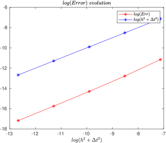
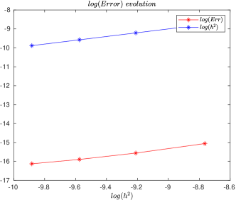
Hence, for some values of the spatial and time discretization parameters, the approximated numerical errors given by (11) are shown in Table 1.

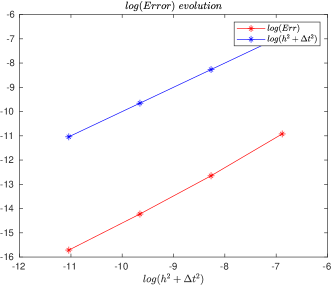
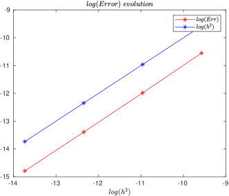
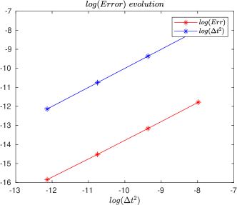
Fig. 1 illustrates how the error depends on the parameters $h^{2}$ and $\Delta t^{2}$ , demonstrating quadratic convergence. This confirms the theoretical results, assuming the solution meets certain regularity conditions. Moreover, Fig. 2 further validates these findings for different cases.

$h\downarrow\Delta t\rightarrow$	0.02	0.01	0.005	0.0025	0.00125
0.02	0.143200720	0.052391942	0.024164654	0.017698156	0.017492619
0.01	0.100412690	0.028129534	0.008809871	0.003280523	0.001545261
0.005	0.090920463	0.023251807	0.006174570	0.001746539	0.000551093
0.0025	0.088623052	0.022107428	0.005592580	0.001442328	0.000384684
0.00125	0.088053433	0.021826038	0.005451913	0.001371276	0.000348277

Table 1. Computed numerical errors

\times 10^{-4}

for a final time

T=1

and for some values of

h

and

\Delta t

Refer to caption — Figure 1. Error behavior on the logarithmic scale.

Case	$h$	$\Delta t$
Case 1: $\Delta t\neq h$	$\tfrac{1}{40}$ , $\tfrac{1}{80}$ , $\tfrac{1}{160}$ , $\tfrac{1}{320}$	$\tfrac{1}{50}$ , $\tfrac{1}{100}$ , $\tfrac{1}{200}$ , $\tfrac{1}{400}$
Case 2: $\Delta t=4h$	$\tfrac{1}{120}$ , $\tfrac{1}{240}$ , $\tfrac{1}{480}$ , $\tfrac{1}{960}$	$\tfrac{1}{30}$ , $\tfrac{1}{60}$ , $\tfrac{1}{120}$ , $\tfrac{1}{240}$
Case 3: $h$ fixed, $\Delta t$ decreasing	$\tfrac{1}{300}$	$\tfrac{1}{54}$ , $\tfrac{1}{108}$ , $\tfrac{1}{216}$ , $\tfrac{1}{432}$
Case 4: $\Delta t$ fixed, $h$ decreasing	$\tfrac{1}{80}$ , $\tfrac{1}{100}$ , $\tfrac{1}{120}$ , $\tfrac{1}{140}$	$\tfrac{1}{700}$

Table 2. Values of

h

and

\Delta t

for different cases.

3.2. Discrete Energy: exponential decay

Now, we consider the system (8) with the following data :

(42)

T=12,\,\alpha=10,\quad\beta=2,\quad\gamma=1,\quad\eta=1,\quad\kappa=1.

and the following initial conditions, for all $x\in(0,1)$ ,

(43)

u_{0}(x)=u_{1}(x)=u_{2}(x)=x^{3}(1-x)^{3},\theta_{0}(x)=x^{2}(1-x)^{2}\sin(x).

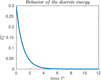
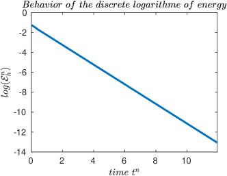
If we take the parameters $3h=\Delta t=0.03$ and we use the following definition for the discrete energy $Math input error$ in Fig. 3(a) and Fig. 3(b) we represent discrete energy and discrete logarithm energy evolution of system $Math input error$ . We can clearly conclude that the discrete energy tends to zero and that an exponential energy decay is achieved.

The numerical schemes were implemented using MATLAB.

References

[1]
[2] Afilal Mounir, Tijani Abdul-Aziz Apalara, Abdelaziz Soufyane and Atika Radid, On the decay of MGT-viscoelastic plate with heat conduction of Cattaneo type in bounded and unbounded domains, Commun. Pure Appl. Anal., 22 (2023), pp. 212–227. https://doi.org/10.3934/cpaa.2022151
[3]
[4] F. Bucci, I. Lasiecka, Feedback control of the acoustic pressure in ultrasonic wave propagation, Optimization 68 (2019), pp. 1811–1854. https://doi.org/10.1080/02331934.2018.1504051
[5] F. Bucci, L. Pandolfi, On the regularity of solutions to the Moore-Gibson-Thompson equation: a perspective via wave equations with memory, J. Evol. Equ., 20 (2020), pp. 837–867. .https://doi.org/10.1007/s00028-019-00549-x
[6] Campo M, Fernández JR, Kuttler KL, Shillor M, Viano JM. Numerical analysis and simulations of a dynamic frictionless contact problem with damage, Comput. Methods Appl. Mech. Eng., 196 (2006) no.1, pp. 476–488. https://doi.org/10.1016/j.cma.2006.05.006
[7] P.G. Ciarlet, The Finite Element Method for Elliptic Problems. In: P.G. Ciarlet, J.L.Lions (eds) Handbook of Numerical Analysis, vol II, North Holland, (1991), pp. 17–352.
[8] M. Conti, V. Pata, M. Pellicer and R. Quintanilla, On the analyticity of the MGT-viscoelastic plate with heat conduction, Journal Diﬀer Equ., 269 (2020), pp. 7862–7880. https://doi.org/10.1016/j.jde.2020.05.043
[9] B. D’Acunto, A. D’Anna, P. Renno, On the motion of a viscoelastic solid in presence of a rigid wall, Z. Angew. Math. Phys., 34 (1983), pp. 421–438. https://doi.org/10.1007/BF00944706
[10] G.C. Gorain, S.K. Bose, Exact controllability and boundary stabilization of torsional vibrations of an internally damped flexible space structure, J. Optim. Theory Appl., 99 (1998), 423–442. https://doi.org/10.1023/A:1021778428222
[11] B. Kaltenbacher, I. Lasiecka, R. Marchand, Wellposedness and exponential decay rates for the Moore-Gibson-Thompson equation arising in high intensity ultrasound, Control Cybern., 40 (2011), pp 971–988.
[12] A.N. Norris, Dynamics of thermoelastic thin plates: a comparison of four theories., J. Therm. Stresses, 29 (2006), pp. 169–195. https://doi.org/10.1080/01495730500257482
[13] R. Marchand, T. McDevitt, R. Triggiani, An abstract semigroup approach to the third-order Moore-Gibson-Thompson partial differential equation arising in high-intensity ultrasound: structural decomposition, spectral anal-ysis, exponential stability, Math. Methods Appl. Sci., 35 (2012), pp. 1896–1929. https://doi.org/10.1002/mma.1576
[14] F.K. Moore, W.E. Gibson, Propagation of weak disturbances in a gas subject to relaxation effects, J. Aerosp. Sci., 27 (1960), pp. 117-–127. https://doi.org/10.2514/8.8418
[15] Professor Stokes, An examination of the possible effect of the radiation of heat on the propagation of sound, Philos. Mag. Ser., 4 (1851), pp. 305–317. https://doi.org/10.1080/14786445108646736
[16] Smouk A., Radid A., Numerical approximation of the MGT system with Fourier’s law, Math. Model. Comput., 11 (2024) no 3, pp. 607-–616 https://doi.org/10.23939/mmc2024.03.607
[17] P.A. Thompson, Compressible-Fluid Dynamics, McGraw-Hill, New York, 1972.
[18]

	$\displaystyle\tfrac{1}{2\Delta t}\left(\left\\|y_{h}^{n}-y_{h}^{n-1}\right\\|^{2%}+\left\\|y_{h}^{n}\right\\|^{2}-\left\\|y_{h}^{n-1}\right\\|^{2}\right)+$
(22)		$\displaystyle\quad+\tfrac{\gamma}{2\alpha\Delta t}\left(\left\\|\Phi_{h}^{n}-%\Phi_{h}^{n-1}\right\\|^{2}+\left\\|\Phi_{h}^{n}\right\\|^{2}-\left\\|\Phi_{h}^{n-%1}\right\\|^{2}\right)$
	$\displaystyle\quad+\tfrac{\nu}{2\alpha\Delta t}\left(\left\\|\Psi_{h}^{n}-\Psi_%{h}^{n-1}\right\\|^{2}+\left\\|\Psi_{h}^{n}\right\\|^{2}-\left\\|\Psi_{h}^{n-1}%\right\\|^{2}\right)+\nu\left\\|\Psi_{h}^{n}\right\\|^{2}$
	$\displaystyle\quad+\tfrac{1}{2\Delta t}\left(\left\\|\theta_{h}^{n}-\theta_{h}^%{n-1}\right\\|^{2}+\left\\|\theta_{h}^{n}\right\\|^{2}-\left\\|\theta_{h}^{n-1}%\right\\|^{2}\right)+\kappa\left\\|\nabla\theta_{h}^{n}\right\\|^{2}=0.$

	$\displaystyle 0$	$\displaystyle=\tfrac{1}{2\Delta t}\left(\left\\|y_{h}^{n}-y_{h}^{n-1}\right\\|^{%2}+\left\\|y_{h}^{n}\right\\|^{2}-\left\\|y_{h}^{n-1}\right\\|^{2}\right)$
		$\displaystyle\quad+\tfrac{\gamma}{2\alpha\Delta t}\left(\left\\|\Phi_{h}^{n}-%\Phi_{h}^{n-1}\right\\|^{2}+\left\\|\Phi_{h}^{n}\right\\|^{2}-\left\\|\Phi_{h}^{n-%1}\right\\|^{2}\right)$
(23)			$\displaystyle\quad+\tfrac{\nu}{2\alpha\Delta t}\left(\left\\|\Psi_{h}^{n}-\Psi_%{h}^{n-1}\right\\|^{2}+\left\\|\Psi_{h}^{n}\right\\|^{2}-\left\\|\Psi_{h}^{n-1}%\right\\|^{2}\right)+\nu\left\\|\Psi_{h}^{n}\right\\|^{2}$
		$\displaystyle\quad+\tfrac{1}{2\Delta t}\left(\left\\|\theta_{h}^{n}-\theta_{h}^%{n-1}\right\\|^{2}+\left\\|\theta_{h}^{n}\right\\|^{2}-\left\\|\theta_{h}^{n-1}%\right\\|^{2}\right)+\kappa\left\\|\nabla\theta_{h}^{n}\right\\|^{2}$
		$\displaystyle\geq\tfrac{\mathcal{E}_{h}^{n}-\mathcal{E}_{h}^{n-1}}{\triangle t}.$

(24)		$\displaystyle\max_{0\leq n\leq N}\left\{\left\\|y^{n}-y_{h}^{n}\right\\|^{2}+%\left\\|\Phi^{n}-\Phi_{h}^{n}\right\\|^{2}+\left\\|\Psi^{n}-\Psi_{h}^{n}\right\\|^%{2}+\left\\|\theta^{n}-\theta_{h}^{n}\right\\|^{2}\right\}\leq$
	$\displaystyle\leq C\Delta t\sum_{i=1}^{N}\left(\left\\|y_{t}^{i}-\delta y^{i}%\right\\|^{2}+\left\\|\Phi_{t}^{i}-\delta\Phi^{i}\right\\|^{2}+\left\\|\Psi_{t}^{i%}-\delta\Psi^{i}\right\\|^{2}+\left\\|\theta_{t}^{i}-\delta\theta^{i}\right\\|^{2%}\right.$
	$\displaystyle\quad\left.+\left\\|\nabla y^{i}-\nabla\chi_{h}^{i}\right\\|^{2}+%\left\\|\nabla\theta^{i}-\nabla\xi_{h}^{i}\right\\|^{2}\right)+C\max_{0\leq n%\leq N}\left\{\left\\|y^{n}-\chi_{h}^{n}\right\\|^{2}+\left\\|\theta^{n}-\xi_{h}^%{n}\right\\|^{2}\right\}$
	$\displaystyle\quad+\tfrac{C}{\Delta t}\sum_{i=1}^{N-1}\left(\left\\|y^{i}-\chi_%{h}^{i}-\left(y^{i+1}-\chi_{h}^{i+1}\right)\right\\|^{2}+\left\\|\theta^{i}-\xi_%{h}^{i}-\left(\theta^{i+1}-\xi_{h}^{i+1}\right)\right\\|^{2}\right)$
	$\displaystyle\quad+C\left(\left\\|y^{0}-y_{h}^{0}\right\\|^{2}+\left\\|\Phi^{0}-%\Phi_{h}^{0}\right\\|^{2}+\left\\|\Psi^{0}-\Psi_{h}^{0}\right\\|^{2}+\left\\|%\theta^{0}-\theta_{h}^{0}\right\\|^{2}\right),$

(32)		$\displaystyle\tfrac{1}{2\Delta t}\left(\left\\|y^{n}-y_{h}^{n}\right\\|^{2}-%\left\\|y^{n-1}-y_{h}^{n-1}\right\\|^{2}\right)+\tfrac{\gamma}{2\alpha\Delta t}%\left(\left\\|\Phi^{n}-\Phi_{h}^{n})\right\\|^{2}-\left\\|\Phi^{n-1}-\Phi_{h}^{n-%1}\right\\|^{2}\right)$
	$\displaystyle\quad\!\!+\!\!\tfrac{\nu}{2\alpha\Delta t}\left(\left\\|\Psi^{n}\!%\!-\!\!\Psi_{h}^{n}\right\\|^{2}\!\!-\!\!\left\\|\Psi^{n-1}\!\!-\!\!\Psi_{h}^{n-%1}\right\\|^{2}\right)\!\!+\!\!\nu\left\\|\Psi^{n}\!\!-\!\!\Psi_{h}^{n}\right\\|^%{2}\!-\!\eta\left(\nabla\theta^{n}\!-\!\nabla\theta_{h}^{n},\nabla y^{n}\!\!-%\!\!\nabla y_{h}^{n}\right)$
	$\displaystyle\leq C\left(\left\\|y_{t}^{n}-\delta y^{n}\right\\|^{2}+\left\\|y^{n%}-y_{h}^{n}\right\\|^{2}+\left\\|\Phi_{t}^{n}-\delta\Phi^{n}\right\\|^{2}+\left\\|%\Phi^{n}-\Phi_{h}^{n})\right\\|^{2}\right.+\left\\|\Psi_{t}^{n}-\delta\Psi^{n}%\right\\|^{2}$
	$\displaystyle\quad\!+\!\left\\|\Psi^{n}\!-\!\Psi_{h}^{n})\right\\|^{2}\!+\!\left%\\|\nabla\theta^{n}\!-\!\nabla\theta_{h}^{n}\right\\|^{2}\!+\!\left\\|y^{n}\!-\!%\chi_{h}\right\\|^{2}+\left\\|\nabla y^{n}-\nabla\chi_{h}\right\\|^{2}\!+\!\left%\\|\Delta y^{n}-\Delta\chi_{h}\right\\|^{2}\left.\right)$
	$\displaystyle\quad+\left(\delta y^{n}-\delta y_{h}^{n},y^{n}-\chi_{h}\right),%\ \text{for all }\chi_{h}\in S_{0}^{h}.$

(33)		$\displaystyle\tfrac{1}{2\Delta t}\left(\left\\|\theta^{n}\!-\!\theta_{h}^{n}%\right\\|^{2}\!-\!\left\\|\theta^{n-1}\!-\!\theta_{h}^{n-1}\right\\|^{2}\right)\!%+\!\kappa\left\\|\nabla\theta^{n}\!-\!\nabla\theta_{h}^{n}\right\\|^{2}\!+\!\eta%\left(\nabla y^{n}\!-\!\nabla y_{h}^{n},\nabla\theta^{n}\!-\!\nabla\theta_{h}^%{n}\right)$
	$\displaystyle\leq C\left(\left\\|\theta_{t}^{n}-\delta\theta^{n}\right\\|^{2}+%\left\\|\theta^{n}-\theta_{h}^{n}\right\\|^{2}+\left\\|\nabla\theta^{n}-\nabla%\theta_{h}^{n}\right\\|^{2}+\left\\|\nabla y^{n}-\nabla y_{h}^{n}\right\\|^{2}+%\left\\|\theta^{n}-\xi_{h}\right\\|^{2}\right.$
	$\displaystyle\quad\left.+\left\\|\nabla\theta^{n}-\nabla\xi_{h}\right\\|^{2}%\right)+\left(\delta\theta^{n}-\delta\theta_{h}^{n},\theta^{n}-\xi_{h}\right).$

Numerical Analysis and Stability of the Moore-Gibson-Thompson-Fourier Model

Abstract.

Key words and phrases:

2005 Mathematics Subject Classification:

1. Introduction

Theorem 1 ([8]).

2. Numerical approximation

Theorem 2.

Proof.

Theorem 3.

Proof.

Corollary 4.

3. Numerical Simulation

3.1. Numerical Convergence: error estimate with an exact solution

3.2. Discrete Energy: exponential decay

References

Information

Indexing and abstracting

Publisher