Additive Operator Splitting Scheme
for a General Mean Curvature Flow
and Application in Edges Enhancement

Rafaa Chouder^∗ and Noureddine Benhamidouche^∗

(Date: October 29, 2024; accepted: November 13, 2024; published online: December 18, 2024.)

Abstract.

Many models that use non-linear partial differential equations (PDEs) have been extensively applied for different tasks in image processing. Among these PDE-based approaches, the mean curvature flow filtering has impressive results, for which feature directions in the image are important.

In this paper, we explore a general model of mean curvature flow, as proposed in [ G.I. Barenblatt, Self-similar intermediate asymptotics for nonlinear degenerate parabolic free-boundary problems that occur in image processing, Proceedings of the National Academy of Sciences of the United States of America (2001)], [ G.I. Barenblatt and J.L. Vazquez, Nonlinear diffusion and image contour enhancement, Interfaces and Free Boundaries (2003)]. The model can be re-arranged to a reaction-diffusion form, facilitating the creation of an unconditionally stable semi-implicit scheme for image filtering. The method employs the Additive Operator Split (AOS) technique. Experiments demonstrated that the modified general model of mean curvature flow is highly effective for reducing noise and has a superior job of preserving edges.

Key words and phrases:

Nonlinear diffusion equations, mean curvature flow, additive operator splitting, unconditionally stable schemes, edge enhancement.

2005 Mathematics Subject Classification:

^∗Laboratory of Pure and Applied Mathematics, University of M’sila, University pole, Road Bordj Bou Arreridj, M’sila 28000, Algeria. rafaa.chouder@univ-msila.dz, noureddine.benhamidouche@univ-msila.dz
This research work is supported by the The General Direction of Scientific Research and Technological Development (DGRSDT)- Algeria.

1. Introduction

Partial differential equation (PDE) based techniques have been widely applied for various image processing tasks over the past few decades [30, 4, 32, 7, 14]. Designing numerical schemes that take into consideration accuracy, stability, and computational cost is fundamental for the effective implementation of these schemes.

Local geometric properties of images are usually dominated by two main directions: the direction perpendicular to the edge, called the flow-line, and parallel to the level or isophote, which is aligned with the edge. By selecting the appropriate degree of diffusion in these two directions, several approaches can be achieved [3, 26, 18, 9, 10].

Mean curvature flow is a prominent example where diffusion only occurs along edges. The theoretical properties of this were first studied by Gage, Hamilton and Huisken in the 1980s [16, 17, 15]. It is known that a plane curve moving at a normal speed equal to its curvature will shrink to a point, its shape becoming smoother and circular. In higher dimensions, the phenomena are more complex, with no classification is available yet. In the context of image processing, Osher and Sethian [22, 27] provided a more rigorous view, realization that the iso-intensity contours of an image can be moved under their curvature was achieved. This led to numerous papers where the images were viewed as a set of level contours, then moved under their curvature. Image smoothing by level-set curvature motion [19, 20] preserves edge information by thwarting diffusion in the edge direction. This work showed that, in addition to this basic approach, a natural stopping criterion can also be chosen to prevent over-smoothing a given image.

A general mathematical framework for feature-preserving image smoothing, applicable to gray-level, vector-value (color) images, volumetric images, and movies was achieved by Sochen, Kimmel, and Malladi in [28, 29]. The main idea is to view the image as a two-dimensional manifold embedded in a hybrid spatial-feature space. The authors in [29] showed that many classical geometric flows emerge as special cases in this view, along with a new flow known as the Beltrami flow, which moves a Gray-level image under a scaled mean curvature. By following a different approach, Yezzi in [33] arrived at a similar equation.

As a result of the certain degeneracy of the asymptotic forms of equations mentioned in [20, 29], Barenblatt [5] noted the possibility of constructing a more general class of equations that generalized mean curvature motion and Beltrami flow. An asymptotic treatment in the one-dimensional case of this class of equations has been investigated theoretically in [5, 6]. The authors report that the general mean curvature flow equation forms a sharp step in the vicinity of edges.

The task of smoothing noisy images and enhancing their edges generally involves solving partial differential equations using numerical integration. This process is often the most time-intensive aspect of nonlinear image processing algorithms. Recently, a lot of research efforts have focused on developing numerical methods and techniques for solving equations dependent on curvature in image processing (see, e.g., [24, 25, 21, 34]).

Our objective is to numerically solve the modified general model of mean curvature flow and to confirm the one-dimension theoretical results obtained in [5]. This is achieved through the development of finite difference schemes for the two-dimensional model. We aim to investigate two critical aspects: The phenomenon of edge enhancement within the image, and the model’s efficacy in noise reduction. Using explicit finite difference schemes can be very time-consuming due to the scaling and small time step requirements in order to achieve stability. Therefore, developing fast and unconditionally stable schemes is preferable. The additive operator splitting (AOS) method, introduced by Weickert et al. [31] for the nonlinear diffusion flow, as an unconditionally stable scheme, is effective and efficient. Applying the (AOS) method in the modified general model of mean curvature flow requires writing the model to allow this method’s application, which we will detail in this paper.

The paper is structured as follows: In Section 2, we present the mathematical model associated to a general mean curvature flow for edge enhancement. Section 3 is devoted to the presentation of the numerical processing, particularly splitting the model and spatial discretization are presented, then the proposed numerical scheme for solving the discretized problem are exposed. Section 4 presents the numerical experiments for image processing. Finally, the paper concludes by a short conclusion.

2. A general mean curvature flow

The level set method [22, 27] elegantly handles mean curvature flow. Essentially, it views the curve as the level set $u=0$ of a function $u$ constrained to solve the degenerate diffusion equation:

(1)

\partial_{t}u=\left|\nabla u\right|\operatorname{div}\left(\tfrac{\nabla u}{%\left|\nabla u\right|}\right),

where $\nabla=\left(\partial_{x},\partial_{y}\right)\$ denotes the gradient operator and $\operatorname{div}$ stands for the divergence operator. To avoid a division by zero, according to [13], a positive parameter is adopted to regularize the term $\left|\nabla u\right|$ . Thus, we have:

(2)		$\displaystyle\partial_{t}u(x,y,t)$	$\displaystyle=$	$\displaystyle\sqrt{1+\left\|\nabla u\right\|^{2}}\operatorname{div}\left(\tfrac{%\nabla u}{\sqrt{1+\left\|\nabla u\right\|^{2}}}\right)$
(2)			$\displaystyle=$	$\displaystyle\tfrac{(1+u_{y}^{2})u_{xx}-2u_{x}u_{y}u_{xy}+(1+u_{x}^{2})u_{yy}}%{1+u_{x}^{2}+u_{y}^{2}},$

which called the mean curvature flow equation.

Sochen et al. [29] used a differential-geometric approach with various assumptions regarding the image intensity flux, leading them to derive the following equation for image intensity $u$

(3)

\partial_{t}u(x,y,t)=\tfrac{(1+u_{y}^{2})u_{xx}-2u_{x}u_{y}u_{xy}+(1+u_{x}^{2}%)u_{yy}}{\left(1+u_{x}^{2}+u_{y}^{2}\right)^{2}},

which called the Beltrami flow (selective mean curvature flow). Here, $x$ and $y$ are the Cartesian coordinates in the image plane, $t$ is time. Thus, according to [20] and [29], image processing is reduced to the solution of the chosen equation under an initial condition $u(x,y,0)=u_{0}(x,y)$ corresponding to a gray level of the image being processed.

As a result of a certain degeneracy of the asymptotic forms of equations $Math input error$ and $Math input error$ , Barenblatt in [5], proposed to consider a more general class of equations

(4)

\partial_{t}u(x,y,t)=\tfrac{(\lambda^{2}+u_{y}^{2})u_{xx}-2u_{x}u_{y}u_{xy}+(%\lambda^{2}+u_{x}^{2})u_{yy}}{\lambda^{-2\alpha}\left(\lambda^{2}+u_{x}^{2}+u_%{y}^{2}\right)^{\alpha+1}},

where $\alpha$ and $\lambda$ are constant parameters $\left(\lambda\neq 0\right)$ . In the other words, it is appropriate to consider a more general flow defined by:

(5)

\partial_{t}u=\left(1+\left|\tfrac{\nabla u}{\lambda}\right|^{2}\right)^{\frac%{1}{2}-\alpha}\operatorname{div}\Bigg{(}\tfrac{\nabla u}{\sqrt{1+\big{|}\tfrac%{\nabla u}{\lambda}\big{|}^{2}}}\Bigg{)}.

Here, the variable $\lambda$ plays the role of a contrast parameter to distinguish between regions to be smoothed and edges to be preserved. For $\left|\nabla u\right|>\lambda$ , edges are preserved, signifying the diffusion effect is small; whereas for $\left|\nabla u\right|<\lambda$ , the diffusion coefficient has a high amplitude, leading to a strong smoothing effect. In other words, regions where $\left|\nabla u\right|>\lambda$ are considered as edges, and the diffusion process has a low effect. Perona and Malik in [23] have pointed out the problem with the setting of $\lambda$ . This presents an interesting problem because a suitable value of the parameter $\lambda$ turns into a general problem of region separation, object extraction, and edge preservation.

Equation $Math input error$ is regard as a generalization of mean curvature flow and the Beltrami flow. To justify this, consider the special case $\alpha=0$ and $\lambda=1,$ to obtain the mean curvature flow equation $Math input error$ , and we can obtain Beltrami flow equation $Math input error$ for $\alpha=1$ . It can be observed that in the case of $\alpha=\frac{1}{2}$ , it is the Perona-Malik diffusion equation with the Charbonier edge indicator function $g(s)=\frac{1}{\sqrt{1+(s/\lambda)^{2}}}$ .

The difference of equation $Math input error$ to mean curvature flow and Beltrami flow is the exponent $\alpha$ on the term $\left(1+\left|\nabla u\right|^{2}\right)^{\frac{1}{2}-\alpha}$ on the right-hand-side. This factor is used for the enhancement of edges. Indeed, it controls the speed of the diffusion: if $\left|\nabla u\right|$ has a small mean in the neighborhood of an interior point of a smooth region of an image, and the diffusion is therefore strong. On the other hand, at the position of an edge, $\left|\nabla u\right|$ is large, the diffusion spread is lowered, since $\left(1+\left|\nabla u\right|^{2}\right)^{\frac{1}{2}-\alpha}$ is small for $\alpha>\frac{1}{2},$ whereas for $\alpha\leq\frac{1}{2}$ , the factor becomes much large then $1$ , this leads to a higher evolution velocity close to an edge.

The asymptotic treatment of this model, for $\alpha=0$ and $\alpha=1,$ done in the papers [20, 29], shows the enhancement of the intensity contrasts by formation of regions of large intensity gradients, i.e., the normal component of the image intensity gradient becomes quite large. This phenomenon was analyzed, for $\alpha\geq 0,$ in [5, 6], where a further 1-D simplification of the model was proposed in order to focus on the boundary layer where large gradients concentrate. Authors proved that the edge enhancement will take place if any equation of class $Math input error$ will be used. In [12, 11] the one-dimensional model have been investigate by using the traveling profiles method proposed in [8].

Solving nonlinear PDEs using explicit methods can be very time consuming due to the scaling and small time step requirement. In this paper our goal is to build a fast and reliable method to solve the general mean curvature flow equation (GMCF) $Math input error$ and it is based on AOS technique by using a semi-implicit finite difference scheme. The mathematical model is achieved by the following additional homogeneous Neumann boundary condition expressing the conservation of energy

\tfrac{\partial u}{\partial n}=0,

where $n$ represents the outward vector normal to the boundary of the domain where the image is defined.

3. Additive Operator Splitting scheme for the general mean curvature flow

To numerically solve equation (5), we utilize the Additive Operator Splitting (AOS) technique, originally introduced by Weickert et al. [31], as an efficient, reliable, and unconditionally stable schemes for nonlinear diffusion in image processing. We adapt the AOS technique to the general mean curvature flow (GMCF), which, although distinct from nonlinear diffusion, can be treated similarly.

Splitting the GMCF

Consider the general mean curvature flow compared with the nonlinear diffusion of a gray-level image. Let $u$ be the pixel value. Equation (5) can be rewritten as:

(6)

\partial_{t}u=h^{\frac{1}{2}-\alpha}\operatorname{div}\left(\tfrac{\nabla u}{%\sqrt{h}}\right),

where

h=1+\left|\tfrac{\nabla u}{\lambda}\right|^{2}=1+\left(\tfrac{u_{x}}{\lambda}%\right)^{2}+\left(\tfrac{u_{y}}{\lambda}\right)^{2}.

To simplify Equation (6), we have:

	$\displaystyle\partial_{t}u$	$\displaystyle=\tfrac{1}{h^{\alpha-1/2}}\left[\tfrac{1}{\sqrt{h}}\left(u_{xx}+u%_{yy}\right)-\tfrac{1}{2}\left(\tfrac{u_{x}h_{x}}{h\sqrt{h}}+\tfrac{u_{y}h_{y}%}{h\sqrt{h}}\right)\right]$
		$\displaystyle=\tfrac{u_{xx}+u_{yy}}{h^{\alpha}}-\tfrac{1}{2}\left(\tfrac{u_{x}%h_{x}}{h^{\alpha+1}}+\tfrac{u_{y}h_{y}}{h^{\alpha+1}}\right)$
		$\displaystyle=\left(1-\tfrac{1}{2\alpha}\right)\tfrac{u_{xx}+u_{yy}}{h^{\alpha%}}+\tfrac{1}{2\alpha}\tfrac{u_{xx}+u_{yy}}{h^{\alpha}}-\tfrac{1}{2}\left(%\tfrac{u_{x}h_{x}}{h^{\alpha+1}}+\tfrac{u_{y}h_{y}}{h^{\alpha+1}}\right)$
		$\displaystyle=\left(1-\tfrac{1}{2\alpha}\right)\tfrac{u_{xx}+u_{yy}}{h^{\alpha%}}+\tfrac{1}{2\alpha}\left\{\tfrac{u_{xx}+u_{yy}}{h^{\alpha}}-\alpha\left(%\tfrac{u_{x}h_{x}}{h^{\alpha+1}}+\tfrac{u_{y}h_{y}}{h^{\alpha+1}}\right)\right\}$
		$\displaystyle=\left(\tfrac{2\alpha-1}{2\alpha}\right)\tfrac{u_{xx}+u_{yy}}{h^{%\alpha}}+\tfrac{1}{2\alpha}\left\{\tfrac{\partial}{\partial x}\left(\tfrac{u_{%x}}{h^{\alpha}}\right)+\tfrac{\partial}{\partial y}\left(\tfrac{u_{y}}{h^{%\alpha}}\right)\right\}.$

We set $g=\frac{1}{h^{\alpha}}$ . By reducing the above equation, we obtain a reaction-diffusion form:

(7)

\partial_{t}u=\tfrac{2\alpha-1}{2\alpha}g\triangle u+\tfrac{1}{2\alpha}\nabla%\left(g\nabla u\right).

In this form, the equation is not a pure diffusion equation. It has both an “parabolic” edge-preserving and an “hyperbolic” edge-sharpening terms. In addition, the reaction-diffusion form of equation $Math input error$ hides the mixed derivative $\partial_{xy}u$ , there by making it conducive to the AOS approach.

In more concise terms, the equation can be rearranged as:

(8)

\partial_{t}u=\left(A_{x}+A_{y}\right)u,

where $A_{x}$ and $A_{y}$ are the following differential operators:

(9)

\left\{\begin{array}[]{c}A_{x}=\frac{1}{2\alpha}\frac{\partial}{\partial x}%\left(g\frac{\partial}{\partial x}\right)+\frac{2\alpha-1}{2\alpha}g\frac{%\partial^{2}}{\partial x^{2}}\\A_{y}=\frac{1}{2\alpha}\frac{\partial}{\partial y}\left(g\frac{\partial}{%\partial y}\right)+\frac{2\alpha-1}{2\alpha}g\frac{\partial^{2}}{\partial y^{2%}}\end{array}\right.

Applying the backward difference formula to $Math input error$ we get,

(10)

\tfrac{U^{q+1}-U^{q}}{dt}=\left(A_{x}+A_{y}\right)U^{q+1}.

Here, the superscript $q$ corresponds to the current time step, while $q+1$ denotes the next time step. The subscripts $i, j$ indicate the discrete pixel location. $U^{q}_{i,j}$ are the known values, and $U^{q+1}_{i,j}$ are the unknown values to be determined. Using $U^{q+1}$ on the right side of $Math input error$ , the integration scheme becomes implicit and unconditionally stable,

(11)

\left[I-dt\left(A_{x}+A_{y}\right)\right]U^{q+1}=U^{q},

where $I$ is the identity matrix. Before proceeding in time, we calculate the values of the edge indicator function $g$ , using the known values of $U^{q}$ . Thus, the scheme is only semi-implicit. Although $g$ depends of the gradient of $U$ , we treat it like a given function of $\left(x,y\right)$ , making the governing PDE “quasi-linear”.

Note that equation $Math input error$ includes a large bandwidth matrix, because all equations related to new pixel values $U^{q+1}$ are coupled. Our aim is to decouple the set $Math input error$ so that each row and each column of pixels can be handled separately. For this, we rearrange the equation into the following form:

(12)

U^{q+1}=\left[I-dt\left(A_{x}+A_{y}\right)\right]^{-1}U^{q}\\=\left[\tfrac{1}{2}\left(I-2dtA_{x}\right)+\tfrac{1}{2}\left(I-2dtA_{y}\right)%\right]^{-1}U^{q}

Of course, we do not intend to invert the matrix to solve the linear set. This is merely a symbolic form used for further derivation.

Equation $Math input error$ is interesting form in the sense that the system matrix is decomposed. The problem is that the decomposed system matrix is inside the $\left[\text{ }\right]^{-1}$ operator. Instead, we aim to construct the solution in parts as follows:

(13)

U^{q+1}=\left(\left[\tfrac{1}{2}\left(I-2dtA_{x}\right)\right]^{-1}+\left[%\tfrac{1}{2}\left(I-2dtA_{x}\right)\right]^{-1}\right)U^{q}

The problem is that the right hand sides of equations $Math input error$ and $Math input error$ are not equal, as can be easily verified. Therefore, we pose the question if there exist a simple variable $m$ , when used to multiplay the right hand side of $Math input error$ , would make them equal:

	$\displaystyle m\left(\left[\tfrac{1}{2}\left(I-2dtA_{x}\right)\right]^{-1}+%\left[\tfrac{1}{2}\left(I-2dtA_{x}\right)\right]^{-1}\right)U^{q}=$
	$\displaystyle=\left[\tfrac{1}{2}\left(I-2dtA_{x}\right)+\tfrac{1}{2}\left(I-2%dtA_{y}\right)\right]^{-1}U^{q}$

This can be simplified into:

m\sum_{i=1}^{i=2}\left[\tfrac{1}{2}\left(I-2dtA_{i}\right)\right]^{-1}U^{q}=%\left[\sum_{i=1}^{i=2}\dfrac{1}{2}\left(I-2dtA_{i}\right)\right]^{-1}U^{q}

Putting $I-2dtA_{i}=B^{-1}$ , we find:

4mB^{-1}=B^{-1}.

Thus we have:

m=\tfrac{1}{4}

Based on this, to use the additive operator splitting scheme given by equation $Math input error$ , we multiply the right hand side by $\dfrac{1}{4}$ , and obtain the following:

U^{q+1}=\tfrac{1}{4}\sum_{i=1}^{i=2}\left[\tfrac{1}{2}\left(I-2dtA_{i}\right)%\right]^{-1}U^{q}=\sum_{i=1}^{i=2}\left[4\dfrac{1}{2}\left(I-2dtA_{i}\right)%\right]^{-1}U^{q}

which is the same as:

U^{q+1}=\left(2I-4dtA_{x}\right)^{-1}U^{q}+\left(2I-4dtA_{y}\right)^{-1}U^{q}.

Now, the whole idea of this scheme is to bring the equation to a simpler form, allowing us to use efficient block-wise solvers, such as Tri-diagonal matrix algorithm.

Introducing the notations $V=\left(2I-4dtA_{x}\right)^{-1}U^{q}$ and $W=\left(2I-4dtA_{y}\right)^{-1}U^{q}$ . The solution now includes two components:

(14)

U^{q+1}=V+W.

We finally obtain the equation sets for $V$ and $W$ as follows:

(15)

\left\{\begin{array}[]{c}\left(2I-4dtA_{x}\right)V=U^{q}\\\left(2I-4dtA_{y}\right)W=U^{q}\end{array}\right.

The differential operators $A_{x}$ and $A_{y}$ are similar, hence we derive here the difference equation for a single row of pixels. Equation for the column of pixels is identical. Consider a row with $N+1$ pixels enumerated from $0$ to $N$ .

Discretisation

To discretize the first derivative, we approximate it using a centered finite difference scheme as follows:

\begin{array}[]{c}\left(\tfrac{\partial V}{\partial x}\right)_{i+1/2}=\tfrac{V%_{i+1}-V_{i}}{dx}+\mathcal{O}\left(h_{x}^{2}\right)\\\left(\tfrac{\partial V}{\partial x}\right)_{i-1/2}=\tfrac{V_{i}-V_{i-1}}{dx}+%\mathcal{O}\left(h_{x}^{2}\right)\end{array}

For the classical finite difference approximation of the second derivative, we utilize the classical three points scheme:

\left(\tfrac{\partial^{2}V}{\partial x^{2}}\right)_{i}=\tfrac{V_{i+1}-2V_{i}+V%_{i-1}}{dx^{2}}+\mathcal{O}\left(h_{x}^{2}\right).

Note that the omitted error terms are of order $h_{x}^{2}$ .

(16)

4\left(A_{x}V\right)_{i}=\tfrac{2}{\alpha}\left[\tfrac{g_{i+1/2}\left(V_{i+1}-%V_{i}\right)-g_{i-1/2}\left(V_{i}-V_{i-1}\right)}{h_{x}^{2}}+\left(2\alpha-1%\right)g_{i}\tfrac{V_{i+1}-2V_{i}+V_{i-1}}{h_{x}^{2}}\right]

To avoid establishing the values of the edge indicator function $g$ at non-nodal points $i-1/2$ and $i+1/2$ , we average the values of the two neighbour nodes:

(17)

g_{i+1/2}=\frac{g_{i+1}+g_{i}}{2},\text{ and }g_{i-1/2}=\frac{g_{i-1}+g_{i}}{2}

Substituting these averages into the equation (16), we get

(18)		$\displaystyle 4\left(A_{x}V\right)_{i}$	$\displaystyle=\tfrac{1}{\alpha h_{x}^{2}}\Big{[}\left(g_{i-1}+\left(4\alpha-1%\right)g_{i}\right)V_{i-1}-$
		$\displaystyle\quad-\left(g_{i-1}+g_{i+1}+2\left(4\alpha-1\right)g_{i}\right)V_%{i-1}+\left(g_{i+1}+\left(4\alpha-1\right)g_{i}\right)V_{i+1}\Big{]}$

Denote:

\beta_{i}=\tfrac{dt}{\alpha h_{x}^{2}}\left(g_{i-1}+\left(4\alpha-1\right)g_{i%}\right),\text{ and }\gamma_{i}=\tfrac{dt}{\alpha h_{x}^{2}}\left(g_{i+1}+%\left(4\alpha-1\right)g_{i}\right)

From equation (15) and the above expression (18), the finite difference equation becomes

(19)

-\beta_{i}V_{i-1}^{q+1}+(2+\beta_{i}+\gamma_{i})V_{i}^{q+1}-\gamma_{i}V_{i+1}^%{q+1}=U_{i}^{q}

At each time step, we solve an algebraic system where the matrix $\left(2I-4dtA_{x}\right)$ is an irreducible strictly diagonal dominant matrix and then invertible. Such a system can be efficiently solved using block-wise solvers, such as the Tri-diagonal matrix algorithm. Moreover, by using the Von-Neumann method, we can demonstrate that this semi-implicit scheme is unconditionally stable.

A similar equation holds for $W$ in $y-$ dimension for $j=0,1,...M$ .

(20)

-\beta_{j}V_{j-1}^{q+1}+(2+\beta_{j}+\gamma_{j})V_{j}^{q+1}-\gamma_{j}V_{j+1}^%{q+1}=U_{j}^{q}

where

\beta_{j}=\tfrac{dt}{\alpha h_{y}^{2}}\left(g_{j-1}+\left(4\alpha-1\right)g_{j%}\right),\text{ and }\gamma_{j}=\frac{dt}{\alpha h_{y}^{2}}\left(g_{j+1}+\left%(4\alpha-1\right)g_{j}\right)

For the first and last nodes, the Neumann boundary conditions hold:

V_{0}=V_{1}\text{, }V_{N}=V_{N-1}\qquad\text{ and }\qquad W_{0}=W_{1}\text{, }%W_{M}=W_{M-1}.

4. Numerical experiment

In this section, we examine the impact of the model (5) presented in this paper on a diverse range of gray scale images. Additionally, we compare the results obtained with those from the Perona-Malik (for $\alpha=1/2$ ), and Beltrami flow (for $\alpha=1$ ) models, highlighting the model’s efficacy in enhancing edges and reducing noise. All numerical experiments were conducted using the AOS method with $h_{x}=h_{y}=1$ and $dt=1$ .

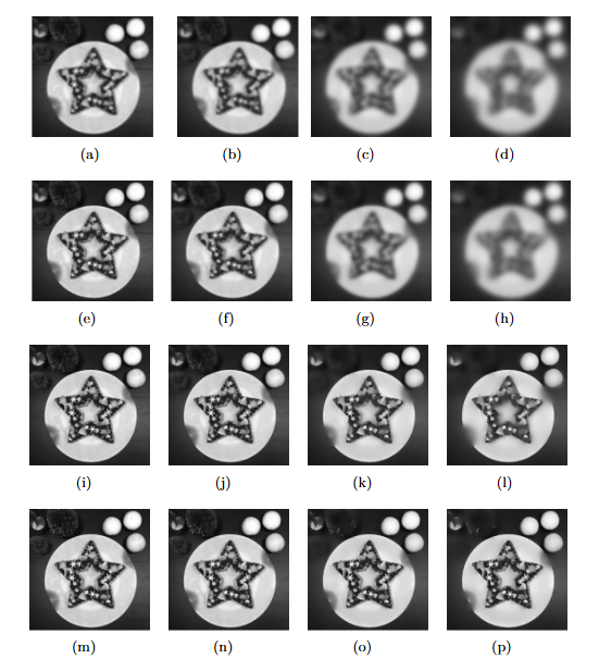
The images in Fig. 1 demonstrate the effects of diffusion at different values of the contrast parameter $\lambda$ . For small values $\lambda$ , the image is smoothed while preserving details better than with larger values of $\lambda$ . In the first line, even if we see that the PM model has a nice edge enhancement property, we have to take into account the importance of the contrast coefficient $\lambda$ , to which the diffusion coefficient is sensitive. Therefore, the problem of determining the value of $\lambda$ is interesting because the appropriate value of $\lambda$ turns into a general problem of region separation, object extraction, and edge preservation. In the second and third lines, it is evident that the images obtained with the Beltrami flow and the general model for $\alpha=2$ are clearer than those obtained with the PM model. Therefore, larger values of the exponent $\alpha$ have done a superior job of preserving edges, even for large values of the contrast parameter $\lambda$ .

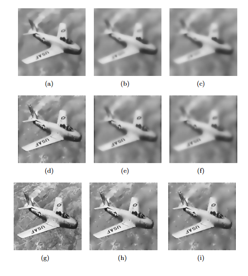
Although a larger number of iterations were required to achieve an equivalent level of smoothing for larger values of $\alpha$ , the improvement in edge preservation can be seen very clearly by looking at the letters in the airplane wing (Fig. 2).

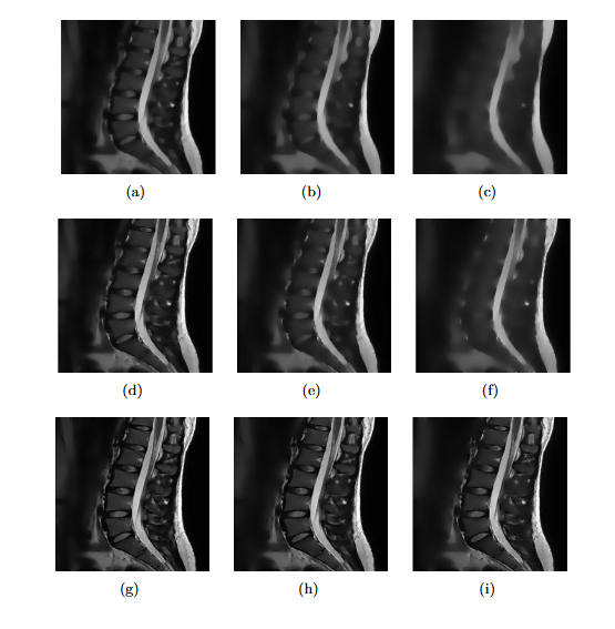
From the images in Fig. 3, one can easily see that the larger exponent $\alpha$ again done a superior job of preserving edges, even for a large number of iterations.

As a conclusion from the experiments presented, it can be said that larger values of $\alpha$ lead to sharper edges, small values lead to smoothed edges, and medium values of $\alpha$ lead to compatibility between the two phenomena. The choice of the value of $\alpha$ remains according to the application and the results to be obtained.

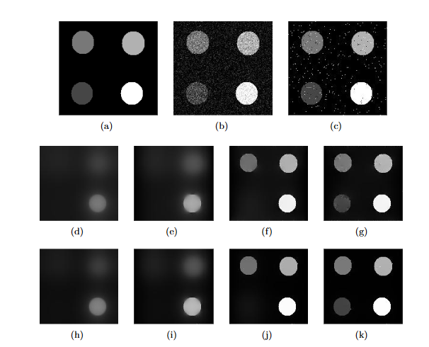
The second simulation concerned the efficacy of the model studied in reducing noise. Experiments were conducted on distorted images with a Gaussian and salt-and-pepper noise. Fig. 4 and Fig. 5 show how noise reduction and edge preservation can be combined using this model. We can observe that it is possible to obtain sharp edges even after a large number of iterations for the large values of $\alpha$ .

Refer to caption — Figure 1. Comparison of different filtering models. Rows from top to bottom: PM model ( $\alpha=0.5$ ), Beltrami flow ( $\alpha=1$ ), GMCF $Math input error$ for $\alpha=2$ ,GMCF $Math input error$ for $\alpha=3$ . Column from Left to Right: $\lambda=1,2,4,6$ . Results after 50 iterations.

5. Conclusion

In this study, we re-arrange the governing equation for the modified general model of mean curvature flow proposed in [5, 6] into a reaction-diffusion form, where the reaction and diffusion terms are explicitly represented. This reaction-diffusion form enables the development of an unconditionally stable semi-implicit scheme for image filtering. The method is based on the Additive Operator Split (AOS), originally applied by Weickert [31] for the nonlinear diffusion flow. The values of the edge indicator function are used from the previous step in scale, while the pixel values of the next step approximate the flow. This approach leads to a semi-implicit linearized difference scheme. The computational time required for image filtering can be reduced by up to ten times or even more compared to the explicit scheme, depending on the scale step value, with no loss of accuracy. Whereas, using explicit finite difference schemes can be very time-consuming due to the scaling and small time-step requirements in order to achieve stability.

Experiments have demonstrated that the modified general model of mean curvature flow is highly effective in reducing noise and excels in edges preservation for large values of exponent $\alpha$ .

References

- [1]
- [2] H. Achour, R. Chouder. N. Benhamidouche, Self-similar solutions for a new free-boundary problem and image contour enhancement, Dynamics of Continuous, Discrete and Impulsive Systems. Series B: Applications & Algorithms, 31 (2024), pp. 321–337. https://online.watsci.org/abstract_pdf//2024v31/v31n5b-pdf/3.pdf
- [3] L. Alvarez, P.L. Lions, J.M. Morel, Image selective smoothing and edge detection by nonlinear diffusion, II, SIAM J. Numer. Anal., 29 (1992), pp. 845–866. https://doi.org/10.1137/0729052
- [4] G. Aubert, and P. Kornprobst, Mathematical Problems in Image Processing - Partial Differential Equations and the Calculus of Variations, Springer, Berlin, 2002.
- [5] G.I. Barenblatt, Self-similar intermediate asymptotics for nonlinear degenerate parabolic free-boundary problems that occur in image processing, Proceedings of the National Academy of Sciences of the United States of America, 98 (2001) no. 23, pp. 12878-12881. https://doi.org/10.1073/pnas.241501698
- [6] G.I. Barenblatt and J.L. Vazquez, Nonlinear diffusion and image contour enhancement, Interfaces and Free Boundaries, 6 (2003) no. 1, pp. 31-54. https://doi.org/10.4171/IFB/90
- [7] S. Benalia and M. Hachama, A nonlocal method for image shadow removal, Computers & Mathematics with Applications, 107 (2022), pp. 95-103. https://doi.org/10.1016/j.camwa.2021.12.023
- [8] N. Benhamidouche, Exact solutions to some nonlinear PDEs, travelling profiles method, Electronic Journal of Qualitative Theory of Differential Equations, (2008), pp. 1–7. https://www.math.u-szeged.hu/ejqtde/p305.pdf
- [9] F. Cao, Geometric Curve Evolution and Image Processing, Volume 1805 of Lecture Notes in Mathematics, Springer, Berlin, 2003.
- [10] V. Caselles, J.-M. Morel, G. Sapiro, and A. Tannenbaum, Introduction to the special issue on partial differential equations and geometry-driven diffusion in image processing and analysis, IEEE Trans. Image Process., 7 (1998) no. 3, pp. 269–273. https://doi.org/10.1109/TIP.1998.661176
- [11] R. Chouder and N. Benhamidouche, New exact solutions to nonlinear diffusion equation that occurs in image processing, International Journal of Computing Science and Mathematics, 10 (2019) no. 4, pp. 364-374. https://doi.org/10.1504/IJCSM.2019.10024353
- [12] R. Chouder and N. Benhamidouche, Travelling profile solutions for nonlinear degenerate parabolic equation and contour enhancement in image processing, Applied Mathematics E-Notes, 18 (2018), pp. 1-12. https://www.emis.de/journals/AMEN/2018/AMEN-161013.pdf
- [13] L.C. Evans and J. Spruck, Motion of level sets by mean curvature I, J. Differ. Geom., 33 (1991) no. 3, pp. 635–681. https://doi.org/10.1007/BF02921385
- [14] M. Hachama, and F. Boutaous, A fractional osmosis model for image fusion, Advances in Computational Mathematics, 50 (2024) no. 7.
- [15] G. Huisken, Flow by mean curvature of convex surfaces into spheres, Journal of Differential Geometry, 20 (1984), pp. 237-266. https://doi.org/10.4310/jdg/1214438998
- [16] M. Gage, Curve shortening makes convex curves circular, Inventions Mathematica, 76 (1984), pp. 357-364.
- [17] M. Gage and R. S. Hamilton, The heat equation shrinking convex plane curves, Journal of Differential Geometry, 23 (1986), pp. 69-96. https://doi.org/10.4310/jdg/1214439902
- [18] R. Kimmel, Numerical Geometry of Images: Theory, Algorithms, and Applications, Springer, New York, 2003.
- [19] R. Malladi and J. A. Sethian, Image processing via level set curvature flow, Proc. of Natl. Acad. of Scie., 92 (1995), pp. 7046–7050. https://doi.org/10.1073/pnas.92.15.7046
- [20] R. Malladi and J. A. Sethian, Image Processing: Flows under Min/Max curvature and Mean Curvature, Graphical Models and Image Processing, 58 (1996) no. 2, pp. 127-141.
- [21] M. Mondelli and A. Ciomaga, Finite difference schemes for MCM and AMSS, Image Processing On Line, 1 (2011).
- [22] S. J. Osher and J. A. Sethian, Fronts propagation with curvature dependent speed: Algorithms based on Hamilton-Jacobi formulations, J. Comput. Phys., 79 (1988), pp. 12–49. https://doi.org/10.5201/ipol.2011.cm_fds
- [23] P. Perona and J. Malik, Scale-space and edge detection using anisotropic diffusion, IEEE Trans. Pattern Anal. Mach. Intell., 12 (1990) no. 7, pp. 629–639. https://doi.org/10.1109/34.56205
- [24] G. Rosman, L. Dascal, A. Sidi, and R. Kimmel, Efficient Beltrami image filtering via vector extrapolation methods, SIAM J. Img. Sci., 2 (2009) no. 3, pp. 858–878. https://doi.org/10.1137/080728391
- [25] G. Rosman, L. Dascal, X. C. Tai and R. Kimmel, On semi-implicit splitting schemes for the Beltrami color image filtering , J. Math. Image. Vision, 40 (2011) no. 2, pp. 199–213. https://doi.org/10.1007/s10851-010-0254-y
- [26] G. Sapiro, Geometric Partial Differential Equations and Image Analysis, Cambridge University Press, Cambridge, UK, 2001. https://doi.org/10.1017/S0025557200173504
- [27] J. A. Sethian, An Analysis of Flame Propagation, Ph. D. Dissertation, University of California, 1982.
- [28] N. Sochen, R. Kimmel and R.Malladi, From high energy physics to low level vision, LBNL Report # 39243, Lawrence Berkeley National Laboratory, University of California, Berkeley, 1996.
- [29] N. Sochen, R. Kimmel and R. Malladi, A general framework for low level vision, IEEE Transactions on Image Processing, 7 (1998) no. 3, pp. 310–318. https://doi.org/10.1109/83.661181
- [30] J. Weickert, Anisotropic Diffusion in Image Processing, B. G. Teubner, Stuttgart, 1998.
- [31] J. Weickert, B.M. ter Haar Romeny and M.A. Viergever, Efficient and reliable scheme for nonlinear diffusion filtering, IEEE Trans on Image Processing, 7 (1998) no. 3, pp. 398-410. https://doi.org/10.1109/83.661190
- [32] M. Welk, and J. Weickert, PDE evolutions for M-smoothers in one, two, and three dimensions, Journal of Mathematical Imaging and Vision, 42 (2021) no. 2, pp. 157-185. https://doi.org/10.1007/s10851-020-00986-1
- [33] A. Yezzi, Modified curvature motion for image smoothing and enhancement, IEEE Transactions on Image Processing, 7 (1998) no. 3, pp. 345–352. https://doi.org/10.1109/83.661184
- [34] J. Zhang, K. Chen, F. Chen and B. Yu, An efficient numerical method for mean curvature-based image registration model, East Asian Journal on Applied Mathematics, 7 (2017) no. 1, pp. 125–142. https://doi.org/10.4208/eajam.200816.031216a