Applications of the theory of generalized Fourier transforms to Tikhonov problems

Abstract.

In this paper, we consider the Sturm-Liouville operator

$${\mathrm{\Delta }}_{SL}:=\frac{{\text{d}}^2}{\text{d}{x}^2}+\frac{A^{\prime }(x)}{A(x)}\frac{\text{d}}{\text{d}x},x\in {ℝ}_{+}^{\ast },$$

where $A$ is a positive function satisfying certain conditions. This operator was used to introduce the generalized Weinstein operator

$${\mathrm{\Delta }}_{GW}:=\frac{{\text{d}}^2}{\text{d}{x}_1^2}+\frac{{\text{d}}^2}{\text{d}{x}_2^2}+\frac{A^{\prime }(x_2)}{A(x_2)}\frac{\text{d}}{\text{d}{x}_2},(x_1,x_2)\in ℝ\times {ℝ}_{+}^{\ast }.$$

We define and study the multiplier operators $T_m^{SL}$ and $T_m^{GW}$ associated with the operators ${\mathrm{\Delta }}_{SL}$ and ${\mathrm{\Delta }}_{GW}$, next, we introduce and study the extremal functions $f_{\eta ,h}^{\ast ,SL}$ and $f_{\eta ,h}^{\ast ,GW}$. The special cases $f_{0,h}^{\ast ,SL}$ and $f_{0,h}^{\ast ,GW}$ are the solutions of a Tikhonov problems.

We present the numerical results associated with $f_{0,h}^{\ast ,SL}$ and $f_{0,h}^{\ast ,GW}$ in two versions. The first is in two dimensions, related to the operator ${\mathrm{\Delta }}_{SL}$, and the second in three dimensions, related to the operator ${\mathrm{\Delta }}_{GW}$.

1. Introduction

Let $E$ be an arbitrary set and let $H_K$ be a reproducing kernel Hilbert space admitting the reproducing kernel $K$ on $E$. For any Hilbert space $H$ we consider a bounded linear operator $T$ from $H_K$ to $H$. Then the following problem is a classical and fundamental problem which is known as best approximate mean square norm problems

(1) $$\underset{f\in H_K}{inf}\left\{{\Vert T(f)-h\Vert }_H^2\right\},$$

where $h\in H$ is given. If there exists $f_h^{\ast }\in H_K$ which attains this infimum, the problem (1) is called solvable otherwise it is called unsolvable. If $H_K$ is a reproducing kernel Hilbert space admitting a reproducing kernel $K(p,q)$ on a the set $E$ then whether the problem (1) is solvable or not, the following problem

(2) $$\underset{f\in H_K}{inf}\{\eta \Vert {f\parallel }_{H_K}^2+{\Vert T(f)-h\Vert }_H^2\},$$

is always solvable for all $\eta >0$ and we obtain a method for determine the extremal function $f_{\eta ,h}^{\ast }\in H_K$ which attains the infimum (2).

The problem (2) is called the Tikhonov regularization for the problem (1) and if the problem (1) is solvable then we have

$$f_{\eta ,h}^{\ast }⟶f_h^{\ast }\text{as}\eta ⟶0^{+},$$

in $H_K$ and $f_h^{\ast }$ is the element which attaints the infimum (1).

In the first part of this paper, we consider the Sturm-Liouville operator (SL-operator) defined by

$${\mathrm{\Delta }}_{SL}:=\frac{{\text{d}}^2}{\text{d}{x}^2}+\frac{A^{\prime }}{A}(x)\frac{\text{d}}{\text{d}x},x\in {ℝ}_{+}^{\ast },$$

where $A$ is a positive function satisfying certain conditions. This operator is the goal of many works in harmonic analysis [2, 3, 6, 7, 4, 24, 25, 26]. Specifically, we consider the Sturm-Liouville transform (SL-transform)

$${ℱ}_{SL}(f)(\lambda ):={\int }_0^{\mathrm{\infty }}{\phi }_{\lambda }^{SL}(x)f(x)A(x)\text{d}x,\lambda \in {ℝ}_{+},$$

where ${\phi }_{\lambda }^{SL}$ is the Sturm-Liouville kernel (SL-kernel) given in Section 2 below. The SL-transform can be considered as a generalization of certain generalized Fourier transforms [5, 8, 9, 11]. Many results have already been demonstrated for the SL-transform ${ℱ}_{SL}$ (see [10, 15, 16, 17, 18, 19, 22, 23]).

We define the Paley-Wiener type space ${𝒫}_s^{SL}$, $s>0$, associated with the SL-transform ${ℱ}_{SL}$, as

$${𝒫}_s^{SL}:={ℱ}_{SL}^{-1}({\chi }_s{L}^2(\nu )),$$

where $L^2(\mu )$ and $L^2(\nu )$ are the Lebesgue spaces defined in Section 2 and ${\chi }_s:={\chi }_{(0,1/s)}$ is the characteristic function of the interval $(0,1/s)$.

In Fourier analysis, a multiplier operator is a type of linear operator, or transformation of functions. The Fourier multiplier operators gave a generalization of some classical linear transformations like, the Hilbert transform, the partial sum operator, the Weierstrass transform and the Poisson integral operator, and recently these operators are the goal of many works [20, 21]. Another fundamental tool in harmonic analysis is the Sturm-Liouville multiplier operators (SL-multiplier operators) which are the aim of the study of this paper.

Let $m\in L^{\mathrm{\infty }}(\nu )$. We define the SL-multiplier operators $T_m^{SL}$ for $f\in L^2(\mu )$, by

$$T_m^{SL}(f):={ℱ}_{SL}^{-1}(m{ℱ}_{SL}(f)).$$

Let $m\in L^{\mathrm{\infty }}(\nu )$. The main goal of the paper is to study the Tikhonov regularization problem

$$\underset{f\in {𝒫}_s^{SL}}{inf}\{\eta \Vert {f\parallel }_{{𝒫}_s^{SL}}^2+{\Vert h-T_m^{SL}(f)\Vert }_{L^2(\mu )}^2\},$$

where $h\in L^2(\mu )$ and $\eta >0$. First this problem has a unique solution (see [12]) denoted by $f_{\eta ,h}^{\ast ,SL}$ and is given by

$$f_{\eta ,h}^{\ast ,SL}(y):={(\eta I+T_m^{SL,\ast }{T}_m^{SL})}^{-1}{T}_m^{SL,\ast }(h)(y),y\in {ℝ}_{+},$$

where $I$ is the unit operator and $T_m^{SL,\ast }:L^2(\mu )\to {𝒫}_s^{SL}$ is the adjoint of $T_m^{SL}$.

Next, by using the theory of the SL-transform ${ℱ}_{SL}$, we prove that the extremal function $f_{\eta ,h}^{\ast ,SL}$ satisfies the following properties.

(i) $T_m^{SL}(f_{\eta ,h}^{\ast ,SL})(y)={\displaystyle {\int }_{{ℝ}_{+}}}\frac{{\chi }_s(\lambda ){\phi }_{\lambda }^{SL}(y){|m(\lambda )|}^2{ℱ}_{SL}(h)(\lambda )}{\eta +{|m(\lambda )|}^2}\text{d}\nu (\lambda )$,

(ii) $T_m^{SL}(f_{\eta ,h}^{\ast ,SL})(y)=f_{\eta ,T_m^{SL}(h)}^{\ast ,SL}(y)$,

(iii) ${lim}_{\eta \to 0^{+}}{\Vert T_m^{SL}(f_{\eta ,h}^{\ast ,SL})-S_s^{SL}(h)\Vert }_{L^2(\mu )}=0$,

(iv) ${lim}_{\eta \to 0^{+}}{T}_m^{SL}(f_{\eta ,h}^{\ast ,SL})(y)=S_s^{SL}(h)(y)$, $y\in {ℝ}_{+}$,
where $S_s^{SL}$ is the partial sum operator associated with the SL-transform ${ℱ}_{SL}$.

In the second part of this paper, we continue the study of the extremal function associated with the generalized Weinstein operator (GW-operator)

$${\mathrm{\Delta }}_{GW}:=\frac{{\text{d}}^2}{\text{d}{x}_1^2}+{{\mathrm{\Delta }}_{SL}|}_{x_2},(x_1,x_2)\in ℝ\times {ℝ}_{+}^{\ast }.$$

This operator provides another view of the Tikhonov regularization problem in two dimensions. Let ${\mu }^{\prime }$ and ${\nu }^{\prime }$ the measures on $𝕂:=ℝ\times {ℝ}_{+}$ given by

$$\text{d}{\mu }^{\prime }(x_1,x_2):=\text{d}{x}_1\text{d}\mu (x_2),\text{d}{\nu }^{\prime }({\lambda }_1,{\lambda }_2):=\frac{1}{2\pi }\text{d}{\lambda }_1\text{d}\nu ({\lambda }_2).$$

The generalized Weinstein transform ${ℱ}_{GW}$ (GW-transform) is defined for $f\in L^1({\mu }^{\prime })$ by

$${ℱ}_{GW}(f)({\lambda }_1,{\lambda }_2):={\int }_{𝕂}{\phi }_{{\lambda }_1,{\lambda }_2}^{GW}(x_1,x_2)f(x_1,x_2)\text{d}{\mu }^{\prime }(x_1,x_2),({\lambda }_1,{\lambda }_2)\in 𝕂,$$

where ${\phi }_{{\lambda }_1,{\lambda }_2}^{GW}(x_1,x_2)=e^{-i{\lambda }_1{x}_1}{\phi }_{{\lambda }_2}(x_2)$ is the generalized Weinstein kernel (GW-kernel). This transform satisfies a Plancherel and an inversion formula.

Let $m\in L^{\mathrm{\infty }}({\nu }^{\prime })$. The generalized Weinstein multiplier operators $T_m^{GW}$ (GW-multiplier operators), are defined for $f\in L^2({\mu }^{\prime })$ by

$$T_m^{GW}(f):={ℱ}_{GW}^{-1}(m{ℱ}_{GW}(f)).$$

We define the Paley-Wiener type space ${𝒫}_s^{GW}$, $s>0$, associated with the GW-transform ${ℱ}_{GW}$, as

$${𝒫}_s^{GW}:={ℱ}_{GW}^{-1}({\chi }_s{L}^2({\nu }^{\prime })),$$

where

$${\chi }_s({\lambda }_1,{\lambda }_2):={\chi }_{(-1/s,1/s)}({\lambda }_1){\chi }_{(0,1/s)}({\lambda }_2),({\lambda }_1,{\lambda }_2)\in 𝕂.$$

Let $m\in L^{\mathrm{\infty }}({\nu }^{\prime })$. For any $h\in L^2({\mu }^{\prime })$ and for any $\eta >0$, the Tikhonov regularization problem

$$\underset{f\in {𝒫}_s^{GW}}{inf}\{\eta \Vert {f\parallel }_{{𝒫}_s^{GW}}^2+{\Vert h-T_m^{GW}(f)\Vert }_{L^2({\mu }^{\prime })}^2\},$$

has a unique solution denoted also by $f_{\eta ,h}^{\ast ,GW}$ and is given by

$$f_{\eta ,h}^{\ast ,GW}(y_1,y_2):={(\eta I+T_m^{GW,\ast }{T}_m^{GW})}^{-1}{T}_m^{GW,\ast }(h)(y_1,y_2),(y_1,y_2)\in 𝕂,$$

where $T_m^{GW,\ast }:L^2({\mu }^{\prime })\to {𝒫}_s^{GW}$ is the adjoint of $T_m^{GW}$.

Using the properties of the GW-transform ${ℱ}_{GW}$, the extremal function $f_{\eta ,h}^{\ast ,GW}$ satisfies the following properties.

(i) $T_m^{GW}(f_{\eta ,h}^{\ast ,GW})(y_1,y_2)=$

$={\displaystyle {\int }_{𝕂}}\frac{{\chi }_s({\lambda }_1,{\lambda }_2){\phi }_{{\lambda }_1,{\lambda }_2}^{GW}(y_1,y_2){|m({\lambda }_1,{\lambda }_2)|}^2{ℱ}_{GW}(h)({\lambda }_1,{\lambda }_2)}{\eta +{|m({\lambda }_1,{\lambda }_2)|}^2}\text{d}{\nu }^{\prime }({\lambda }_1,{\lambda }_2)$.

(ii) $T_m^{GW}(f_{\eta ,h}^{\ast ,GW})(y_1,y_2)=f_{\eta ,T_m^{GW}(h)}^{\ast ,GW}(y_1,y_2)$.

(iii) ${lim}_{\eta \to 0^{+}}{\Vert T_m^{GW}(f_{\eta ,h}^{\ast ,GW})-S_s^{GW}(h)\Vert }_{L^2({\mu }^{\prime })}=0$.

(iv) ${lim}_{\eta \to 0^{+}}{T}_m^{GW}(f_{\eta ,h}^{\ast ,GW})(y_1,y_2)=S_s^{GW}(h)(y_1,y_2)$, $(y_1,y_2)\in 𝕂$,
where $S_s^{GW}$ is the partial sum operator associated with the GW-transform ${ℱ}_{GW}$.

In the third part of this paper, we study two examples of Tikhonov problems and give numerical results associated with $f_{0,h}^{\ast ,SL}$ and $f_{0,h}^{\ast ,GW}$ in two versions. The first in two dimensions is related to the Bessel operator

$${\mathrm{\Delta }}_B:=\frac{{\text{d}}^2}{\text{d}{x}^2}+\frac{1}{x}\frac{\text{d}}{\text{d}x},$$

and the second in three dimensions is related to the Weinstein operator

$${\mathrm{\Delta }}_W:=\frac{{\text{d}}^2}{\text{d}{x}_1^2}+\frac{{\text{d}}^2}{\text{d}{x}_2^2}+\frac{1}{x_2}\frac{\text{d}}{\text{d}{x}_2}.$$

The paper is organized as follows. In Section 2 we recall some results about the SL-operator ${\mathrm{\Delta }}_{SL}$ and the SL-transform ${ℱ}_{SL}$. In Section 3 we study two Tikhonov regularization problems associated with the SL-operator ${\mathrm{\Delta }}_{SL}$ and the GW-operator ${\mathrm{\Delta }}_{GW}$, respectively. In the last section we give numerical results related to the Bessel operator ${\mathrm{\Delta }}_B$ and the Weinstein operator ${\mathrm{\Delta }}_W$ when $\alpha =0$.

2. The SL-multiplier operators

We consider the SL-operator ${\mathrm{\Delta }}_{SL}$ defined on ${ℝ}_{+}^{\ast }$ by

$${\mathrm{\Delta }}_{SL}:=\frac{{\text{d}}^2}{\text{d}{x}^2}+\frac{A^{\prime }(x)}{A(x)}\frac{\text{d}}{\text{d}x},$$

where

$$A(x)=x^{2\alpha +1}B(x),\alpha >-1/2,$$

for $B$ a positive, even, infinitely differentiable function on $ℝ$ such that $B(0)=1$. Moreover we assume that $A$ satisfies the following conditions:

(i) $A$ is increasing and $\underset{x\to \mathrm{\infty }}{lim}A(x)=\mathrm{\infty }$.

(ii) ${\displaystyle \frac{A^{\prime }}{A}}$ is decreasing and $\underset{x\to \mathrm{\infty }}{lim}{\displaystyle \frac{A^{\prime }(x)}{A(x)}}=2\rho \ge 0$.

(iii) There exists a constant $\delta >0$ such that

$$\frac{A^{\prime }(x)}{A(x)}=2\rho +e^{-\delta x}D(x),\text{ if }\rho >0,$$

$$\frac{A^{\prime }(x)}{A(x)}=\frac{2\alpha +1}{x}+e^{-\delta x}D(x),\text{ if }\rho =0,$$

where $D$ is an infinitely differentiable function on ${ℝ}_{+}^{\ast }$, bounded and with bounded derivatives on all intervals $[x_0,\mathrm{\infty })$, for $x_0>0$.

This operator was studied in [4, 24], and the following results have been established:

(I) For all $\lambda \in ℂ$, the equation

admits a unique solution, denoted by ${\phi }_{\lambda }^{SL}$, with the following properties:

$\bullet$ for $x\in {ℝ}_{+}$, the function $\lambda \to {\phi }_{\lambda }^{SL}(x)$ is analytic on $ℂ$;

$\bullet$ for $\lambda \in ℂ$, the function $x\to {\phi }_{\lambda }^{SL}(x)$ is even and infinitely differentiable on $ℝ$.

(II) For nonzero $\lambda \in ℂ$, the equation

$${\mathrm{\Delta }}_{SL}(u)=-({\lambda }^2+{\rho }^2)u,$$

has a solution ${\mathrm{\Phi }}_{\lambda }$ satisfying

$${\mathrm{\Phi }}_{\lambda }(x)=\frac{e^{i\lambda x}}{\sqrt{A(x)}}V(x,\lambda ),$$

with

$$\underset{x\to \mathrm{\infty }}{lim}V(x,\lambda )=1.$$

Consequently there exists a function (spectral function) $\lambda \to c(\lambda )$, such that

$${\phi }_{\lambda }^{SL}(x)=c(\lambda ){\mathrm{\Phi }}_{\lambda }(x)+c(-\lambda ){\mathrm{\Phi }}_{-\lambda }(x),x\in {ℝ}_{+},$$

for nonzero $\lambda \in ℂ$.

Moreover there exist positive constants $k_1$, $k_2$, $k$, such that

$$k_1{|\lambda |}^{2\alpha +1}\le {|c(\lambda )|}^{-2}\le k_2{|\lambda |}^{2\alpha +1},$$

for all $\lambda$ such that $\text{Im}\lambda \le 0$ and $|\lambda |\ge k$.

(III) The SL-function ${\phi }_{\lambda }^{SL}(x)$; $\lambda ,x\in {ℝ}_{+}$, possesses the following property

(3) $$|{\phi }_{\lambda }^{SL}(x)|\le 1.$$

Notation. We denote by

$\bullet$ $\mu$ the measure defined on ${ℝ}_{+}$ by $\text{d}\mu (x):=A(x)\text{d}x$; and by $L^p(\mu )$, $p\in [1,\mathrm{\infty }]$, the space of measurable functions $f$ on ${ℝ}_{+}$, such that

$\bullet$ $\nu$ the measure defined on ${ℝ}_{+}$ by $\text{d}\nu (\lambda ):={\displaystyle \frac{\text{d}\lambda }{2\pi {|c(\lambda )|}^2}}$; and by $L^p(\nu )$, $p\in [1,\mathrm{\infty }]$, the space of measurable functions $f$ on ${ℝ}_{+}$, such that .

The SL-transform is the Fourier transform associated with the operator ${\mathrm{\Delta }}_{SL}$ and is defined for $f\in L^1(\mu )$ by

$${ℱ}_{SL}(f)(\lambda ):={\int }_{{ℝ}_{+}}{\phi }_{\lambda }^{SL}(x)f(x)\text{d}\mu (x),\lambda \in {ℝ}_{+}.$$

Some of the properties of the SL-transform ${ℱ}_{SL}$ are collected bellow (see [4, 24, 25]).

Theorem 1.

• $L^1-L^{\mathrm{\infty }}$-boundedness for ${ℱ}_{SL}$. For all $f\in L^1(\mu )$, ${ℱ}_{SL}(f)\in L^{\mathrm{\infty }}(\nu )$ and

  $${\Vert {ℱ}_{SL}(f)\Vert }_{L^{\mathrm{\infty }}(\nu )}\le {\Vert f\Vert }_{L^1(\mu )}.$$

• Plancherel theorem for ${ℱ}_{SL}$. The SL-transform ${ℱ}_{SL}$ extends uniquely to an isometric isomorphism of $L^2(\mu )$ onto $L^2(\nu )$. In particular,

  $${\Vert f\Vert }_{L^2(\mu )}={\Vert {ℱ}_{SL}(f)\Vert }_{L^2(\nu )}.$$

• Inversion theorem for ${ℱ}_{SL}$. Let $f\in L^1(\mu )$, such that ${ℱ}_{SL}(f)\in L^1(\nu )$. Then

  $$f(x)={\int }_{{ℝ}_{+}}{\phi }_{\lambda }^{SL}(x){ℱ}_{SL}(f)(\lambda )\text{d}\nu (\lambda ),\text{a.e.}x\in {ℝ}_{+}.$$

Let $s>0$ and ${\chi }_s$ be the function defined by

$${\chi }_s(\lambda ):={\chi }_{(0,1/s)}(\lambda ),\lambda \in {ℝ}_{+},$$

where ${\chi }_{(0,1/s)}$ is the characteristic function of the interval $(0,1/s)$.

We define the Paley-Wiener type space ${𝒫}_s^{SL}$, as

$${𝒫}_s^{SL}:={ℱ}_{SL}^{-1}({\chi }_s{L}^2(\nu )).$$

We see that any element $f\in {𝒫}_s^{SL}$ is represented uniquely by a function $F\in L^2(\nu )$ in the form

$$f={ℱ}_{SL}^{-1}({\chi }_{s}F).$$

The space ${𝒫}_s^{SL}$ equipped with the norm

$${\Vert f\Vert }_{{𝒫}_s^{SL}}:={\Vert F\Vert }_{L^2(\nu )}={\left[{\int }_{{ℝ}_{+}}{|F(\lambda )|}^2\text{d}\nu (\lambda )\right]}^{1/2}.$$

Theorem 2.

The space ${𝒫}_s^{SL}$ satisfies

$${ℱ}_{SL}({𝒫}_s^{SL})\subset L^1\cap L^2(\nu ),$$

and has the reproducing kernel

$$K_s(x,y)={\int }_{{ℝ}_{+}}{\chi }_s(\lambda ){\phi }_{\lambda }^{SL}(x){\phi }_{\lambda }^{SL}(y)\text{d}\nu (\lambda ).$$

Proof.

Let $f\in {𝒫}_s^{SL}$. The inclusion follows from the inequality

$${\Vert {ℱ}_{SL}(f)\Vert }_{L^1(\nu )}\le A_s{\Vert f\Vert }_{{𝒫}_s^{SL}},$$

where

$$A_s:={\left[{\int }_{{ℝ}_{+}}{\chi }_s(\lambda )\text{d}\nu (\lambda )\right]}^{1/2}.$$

On the other hand, from Theorem 1 (iii), we have

$${ℱ}_{SL}(K_s(.,y))(\lambda )={\chi }_s(\lambda ){\phi }_{\lambda }^{SL}(y),y\in {ℝ}_{+}.$$

By (3), we get

Moreover,

$${⟨f,K_s(.,y)⟩}_{{𝒫}_s^{SL}}={\int }_{{ℝ}_{+}}{ℱ}_{SL}(f)(\lambda ){\phi }_{\lambda }^{SL}(y)\text{d}\nu (\lambda )=f(y).$$

This completes the proof of the theorem. ∎

Let $m\in L^{\mathrm{\infty }}(\nu )$. The SL-multiplier operators $T_m^{SL}$, are defined for $f\in L^2(\mu )$ by

(4) $$T_m^{SL}(f):={ℱ}_{SL}^{-1}(m{ℱ}_{SL}(f)).$$

Let $m\in L^{\mathrm{\infty }}(\nu )$. By Theorem 1 (ii), the operators $T_m^{SL}$ are bounded from $L^2(\mu )$ into $L^2(\mu )$, and

(5) $${\Vert T_m^{SL}(f)\Vert }_{L^2(\mu )}\le {\Vert m\Vert }_{L^{\mathrm{\infty }}(\nu )}{\Vert f\Vert }_{L^2(\mu )}.$$

Let $m\in L^{\mathrm{\infty }}(\nu )$. By (5), the $SL$-multiplier operators $T_m^{SL}$ are bounded from ${𝒫}_s^{SL}$ into $L^2(\mu )$, and

$${\Vert T_m^{SL}(f)\Vert }_{L^2(\mu )}\le {\Vert m\Vert }_{L^{\mathrm{\infty }}(\nu )}{\Vert f\Vert }_{{𝒫}_s^{SL}}.$$

For example, the partial sum operator $S_s^{SL}$ defined by

$$S_s^{SL}(f):={ℱ}_{SL}^{-1}({\chi }_s{ℱ}_{SL}(f)),$$

is a SL-multiplier operator and satisfies ${\Vert S_s^{SL}(f)\Vert }_{L^2(\mu )}\le {\Vert f\Vert }_{{𝒫}_s^{SL}}$.

Let $\eta >0$. We denote by ${⟨.,.⟩}_{\eta ,{𝒫}_s^{SL}}$ the inner product defined on the space ${𝒫}_s^{SL}$ by

$${⟨f,g⟩}_{\eta ,{𝒫}_s^{SL}}:=\eta {⟨f,g⟩}_{{𝒫}_s^{SL}}+{⟨T_m^{SL}(f),T_m^{SL}(g)⟩}_{L^2(\mu )}.$$

Let $\eta >0$ and let $m\in L^{\mathrm{\infty }}(\nu )$. The space ${𝒫}_s^{SL}$ equipped with the norm $\parallel .{\parallel }_{\eta ,{𝒫}_s^{SL}}$ has the reproducing kernel

$$K_{s,\eta }(x,y)={\int }_{{ℝ}_{+}}\frac{{\chi }_s(\lambda ){\phi }_{\lambda }^{SL}(x){\phi }_{\lambda }^{SL}(y)}{\eta +{|m(\lambda )|}^2}\text{d}\nu (\lambda ).$$

Therefore, we have the functional equation

(6) $$(\eta I+T_m^{SL,\ast }{T}_m^{SL})K_{s,\eta }(.,y)=K_s(.,y),y\in {ℝ}_{+},$$

where $T_m^{SL,\ast }:L^2(\mu )\to {𝒫}_s^{SL}$ is the adjoint of $T_m^{SL}$.

3. Tikhonov regularization problems

In this section, building on the ideas of Saitoh et al. [12, 13, 14], we study and solve the Tikhonov regularization problems associated with the SL-operator and the GW-operator, respectively.

a) Extremal function associated with the SL-operator. For any $h\in L^2(\mu )$ and for any $\eta >0$, the Tikhonov regularization problem

$$\underset{f\in {𝒫}_s^{SL}}{inf}\{\eta \Vert {f\parallel }_{{𝒫}_s^{SL}}^2+{\Vert h-T_m^{SL}(f)\Vert }_{L^2(\mu )}^2\}$$

has a unique solution (see [12]) denoted also by $f_{\eta ,h}^{\ast ,SL}$ and is given by

(7) $$f_{\eta ,h}^{\ast ,SL}(y):={(\eta I+T_m^{SL,\ast }{T}_m^{SL})}^{-1}{T}_m^{SL,\ast }(h)(y),y\in {ℝ}_{+}.$$

This function possesses the following integral representation.

Theorem 3.

Let $m\in L^{\mathrm{\infty }}(\nu )$. Then for any $h\in L^2(\mu )$ and for any $\eta >0$, we have

• $f_{\eta ,h}^{\ast ,SL}(y)={\displaystyle {\int }_{{ℝ}_{+}}}\frac{{\chi }_s(\lambda ){\phi }_{\lambda }^{SL}(y)\overline{m(\lambda )}{ℱ}_{SL}(h)(\lambda )}{\eta +{|m(\lambda )|}^2}\text{d}\nu (\lambda )$.

• ${\Vert f_{\eta ,h}^{\ast ,SL}\Vert }_{{𝒫}_s^{SL}}\le \frac{1}{2\sqrt{\eta }}{\Vert h\Vert }_{L^2(\mu )}$.

Proof.

(i) From Theorem 2, (6) and (7), we have

$f_{\eta ,h}^{\ast ,SL}(y)$ $=$ ${⟨{(\eta I+T_m^{SL,\ast }{T}_m^{SL})}^{-1}{T}_m^{SL,\ast }(h),K_s(.,y)⟩}_{{𝒫}_s^{SL}}$

$=$ ${⟨T_m^{SL,\ast }(h),{(\eta I+T_m^{SL,\ast }{T}_m^{SL})}^{-1}{K}_s(.,y)⟩}_{{𝒫}_s^{SL}}$

$=$ ${⟨T_m^{SL,\ast }(h),K_{s,\eta }(.,y)⟩}_{{𝒫}_s^{SL}}.$

Hence

$$f_{\eta ,h}^{\ast ,SL}(y)={⟨h,T_m^{SL}\left(K_{s,\eta }(.,y)\right)⟩}_{L^2(\mu )}.$$

By (3), the function $\lambda \to {\displaystyle \frac{{\chi }_s(\lambda ){\phi }_{\lambda }^{SL}(y)}{\eta +{|m(\lambda )|}^2}}$ belongs to $L^1\cap L^2(\nu )$. Then from Theorem 1 (ii), it follows that $K_{s,\eta }(.,y)$ belongs to $L^2(\mu )$, and

(8) $${ℱ}_{SL}(K_{s,\eta }(.,y))(\lambda )=\frac{{\chi }_s(\lambda ){\phi }_{\lambda }^{SL}(y)}{\eta +{|m(\lambda )|}^2},y\in {ℝ}_{+}.$$

By Theorem 1 (ii) and (8), we have

$f_{\eta ,h}^{\ast ,SL}(y)$ $=$ ${\displaystyle {\int }_{{ℝ}_{+}}}{ℱ}_{SL}(h)(\lambda )\overline{m(\lambda ){ℱ}_{SL}(K_{s,\eta }(.,y))(\lambda )}\text{d}\nu (\lambda )$

$=$ ${\displaystyle {\int }_{{ℝ}_{+}}}{\displaystyle \frac{{\chi }_s(\lambda ){\phi }_{\lambda }^{SL}(y)\overline{m(\lambda )}{ℱ}_{SL}(h)(\lambda )}{\eta +{|m(\lambda )|}^2}}\text{d}\nu (\lambda ).$

(ii) The function

$$\lambda \to \frac{{\chi }_s(\lambda )\overline{m(\lambda )}{ℱ}_{SL}(h)(\lambda )}{\eta +{|m(\lambda )|}^2},$$

belongs to $L^1\cap L^2(\nu )$. Then by (i), it follows that $f_{\eta ,h}^{\ast ,SL}$ belongs to $L^2(\mu )$, and

(9) $${ℱ}_{SL}(f_{\eta ,h}^{\ast ,SL})(\lambda )=\frac{{\chi }_s(\lambda )\overline{m(\lambda )}{ℱ}_{SL}(h)(\lambda )}{\eta +{|m(\lambda )|}^2}.$$

Since ${\left[\eta +{|m(\lambda )|}^2\right]}^2\ge 4\eta {|m(\lambda )|}^2$, we obtain

${\Vert f_{\eta ,h}^{\ast ,SL}\Vert }_{{𝒫}_s^{SL}}^2$ $=$ ${\displaystyle {\int }_{{ℝ}_{+}}}{\displaystyle \frac{{|m(\lambda )|}^2{|{ℱ}_{SL}(h)(\lambda )|}^2}{{[\eta +{|m(\lambda )|}^2]}^2}}\text{d}\nu (\lambda )$

$\le$ $\frac{1}{4\eta }{\displaystyle {\int }_{{ℝ}_{+}}}{|{ℱ}_{SL}(h)(\lambda )|}^2\text{d}\nu (\lambda )={\displaystyle \frac{1}{4\eta }}{\Vert h\Vert }_{L^2(\mu )}^2.$

The theorem is proved. ∎

In the following we establish some properties for the extremal function $f_{\eta ,h}^{\ast ,SL}$.

Theorem 4.

Let $m\in L^{\mathrm{\infty }}(\nu )$. For any $h\in L^2(\mu )$ and for any $\eta >0$, we have

• $T_m^{SL}(f_{\eta ,h}^{\ast ,SL})(y)={\displaystyle {\int }_{{ℝ}_{+}}}\frac{{\chi }_s(\lambda ){\phi }_{\lambda }^{SL}(y){|m(\lambda )|}^2{ℱ}_{SL}(h)(\lambda )}{\eta +{|m(\lambda )|}^2}\text{d}\nu (\lambda )$.

• $T_m^{SL}(f_{\eta ,h}^{\ast ,SL})(y)=f_{\eta ,T_m^{SL}(h)}^{\ast }(y)$.

• ${lim}_{\eta \to 0^{+}}{\Vert T_m^{SL}(f_{\eta ,h}^{\ast ,SL})-S_s^{SL}(h)\Vert }_{L^2(\mu )}=0$.

• ${lim}_{\eta \to 0^{+}}{T}_m^{SL}(f_{\eta ,h}^{\ast ,SL})(y)=S_s^{SL}(h)(y)$, $y\in {ℝ}_{+}$.

Proof.

By (4) and (9), we have

$$T_m^{SL}(f_{\eta ,h}^{\ast ,SL})(y)={ℱ}_{SL}^{-1}\left({\chi }_s(\lambda )\frac{{|m(\lambda )|}^2{ℱ}_{SL}(h)(\lambda )}{\eta +{|m(\lambda )|}^2}\right)(y).$$

The function

$$\lambda \to {\chi }_s(\lambda )\frac{{|m(\lambda )|}^2{ℱ}_{SL}(h)(\lambda )}{\eta +{|m(\lambda )|}^2}$$

belongs to $L^1\cap L^2(\nu )$. Then by Theorem 1 (iii), we obtain (i).

The (ii) follows from (i) and Theorem 3 (i).

From (i), we have

$${ℱ}_{SL}(T_m^{SL}(f_{\eta ,h}^{\ast ,SL})-S_s^{SL}(h))(\lambda )=-\eta \frac{{\chi }_s(\lambda ){ℱ}_{SL}(h)(\lambda )}{\eta +{|m(\lambda )|}^2}.$$

Consequently,

$${\Vert T_m^{SL}(f_{\eta ,h}^{\ast ,SL})-S_s^{SL}(h)\Vert }_{L^2(\mu )}^2={\int }_{{ℝ}_{+}}\frac{{\eta }^2{\chi }_s(\lambda ){|{ℱ}_{SL}(h)(\lambda )|}^2}{{[\eta +{|m(\lambda )|}^2]}^2}\text{d}\nu (\lambda ).$$

Using the dominated convergence theorem and the fact that

$$\frac{{\eta }^2{\chi }_s(\lambda ){|{ℱ}_{SL}(h)(\lambda )|}^2}{{[\eta +{|m(\lambda )|}^2]}^2}\le {|{ℱ}_{SL}(h)(\lambda )|}^2,$$

we deduce (iii).

Finally, from (i) and Theorem 1 (iii), we deduce that

$$T_m^{SL}(f_{\eta ,h}^{\ast ,SL})(y)-S_s^{SL}(h)(y)=-\eta {\int }_{{ℝ}_{+}}{\phi }_{\lambda }^{SL}(y)\frac{{\chi }_s(\lambda ){ℱ}_{SL}(h)(\lambda )}{\eta +{|m(\lambda )|}^2}\text{d}\nu (\lambda ).$$

Using the dominated convergence theorem and the fact that

$$\frac{\eta {\chi }_s(\lambda )|{ℱ}_{SL}(f)(\lambda )|}{\eta +{|m(\lambda )|}^2}\le {\chi }_s(\lambda )|{ℱ}_{SL}(h)(\lambda )|,$$

we obtain (iv). ∎

b) Extremal function associated with the GW-operator. We consider the GW-operator on $ℝ\times {ℝ}_{+}^{\ast }$ by

$${\mathrm{\Delta }}_{GW}:=\frac{{\text{d}}^2}{\text{d}{x}_1^2}+\frac{{\text{d}}^2}{\text{d}{x}_2^2}+\frac{A^{\prime }(x_2)}{A(x_2)}\frac{\text{d}}{\text{d}{x}_2}=\frac{{\text{d}}^2}{\text{d}{x}_1^2}+{{\mathrm{\Delta }}_{SL}|}_{x_2},(x_1,x_2)\in ℝ\times {ℝ}_{+}^{\ast }.$$

For any $({\lambda }_1,{\lambda }_2)\in 𝕂:=ℝ\times {ℝ}_{+}$, the system

$${\mathrm{\Delta }}_{GW}(u)(x_1,x_2)=-({\lambda }_2^2+{\rho }^2)u(x_1,x_2),$$

$$\frac{{\partial }^{2}u}{\partial x_1^2}(x_1,x_2)=-{\lambda }_1^{2}u(x_1,x_2),$$

$$u(0,0)=1,\frac{\partial u}{\partial x_2}(0,0)=0,\frac{\partial u}{\partial x_1}(0,0)=-i{\lambda }_1.$$

admits a unique solution ${\phi }_{{\lambda }_1,{\lambda }_2}(x_1,x_2)$ given by

$${\phi }_{{\lambda }_1,{\lambda }_2}^{GW}(x_1,x_2)=e^{-i{\lambda }_1{x}_1}{\phi }_{{\lambda }_2}(x_2).$$

For $(x_1,x_2),({\lambda }_1,{\lambda }_2)\in 𝕂$, the kernel ${\phi }_{{\lambda }_1,{\lambda }_2}^{GW}(x_1,x_2)$ satisfies

$$|{\phi }_{{\lambda }_1,{\lambda }_2}^{GW}(x_1,x_2)|\le 1.$$

Notation. We denote by

$\bullet$ ${\mu }^{\prime }$ the measure defined on $𝕂$ by $\text{d}{\mu }^{\prime }(x_1,x_2):=\text{d}{x}_1\text{d}\mu (x_2)$; and by $L^p({\mu }^{\prime })$, $p\in [1,\mathrm{\infty }]$, the space of measurable functions $f$ on $𝕂$, such that .

$\bullet$ ${\nu }^{\prime }$ the measure defined on $𝕂$ by $\text{d}{\nu }^{\prime }({\lambda }_1,{\lambda }_2):=\frac{1}{2\pi }\text{d}{\lambda }_1\text{d}\nu ({\lambda }_2)$; and by $L^p({\nu }^{\prime })$, $p\in [1,\mathrm{\infty }]$, the space of measurable functions $f$ on ${ℝ}_{+}$, such that .

The generalized Weinstein transform is the Fourier transform associated with the operator ${\mathrm{\Delta }}_{GW}$ and is defined for $f\in L^1({\mu }^{\prime })$ by

$${ℱ}_{GW}(f)({\lambda }_1,{\lambda }_2):={\int }_{𝕂}{\phi }_{{\lambda }_1,{\lambda }_2}^{GW}(x_1,x_2)f(x_1,x_2)\text{d}{\mu }^{\prime }(x_1,x_2),({\lambda }_1,{\lambda }_2)\in 𝕂.$$

This transform satisfies the following properties.

Theorem 5.

• $L^1-L^{\mathrm{\infty }}$-boundedness for ${ℱ}_{GW}$. For all $f\in L^1({\mu }^{\prime })$, ${ℱ}_{GW}(f)\in L^{\mathrm{\infty }}({\nu }^{\prime })$ and

  $${\Vert {ℱ}_{GW}(f)\Vert }_{L^{\mathrm{\infty }}({\nu }^{\prime })}\le {\Vert f\Vert }_{L^1({\mu }^{\prime })}.$$

• Plancherel theorem for ${ℱ}_{GW}$. The Weinstein transform ${ℱ}_{GW}$ extends uniquely to an isometric isomorphism of $L^2({\mu }^{\prime })$ onto $L^2({\nu }^{\prime })$. In particular,

  $${\Vert f\Vert }_{L^2({\mu }^{\prime })}={\Vert {ℱ}_{GW}(f)\Vert }_{L^2({\nu }^{\prime })}.$$

• Inversion theorem for ${ℱ}_{GW}$. Let $f\in L^1({\mu }^{\prime })$, such that ${ℱ}_{GW}(f)\in L^1({\nu }^{\prime })$. Then

  $$f(x)={\int }_{𝕂}{\phi }_{{\lambda }_1,{\lambda }_2}^{GW}(x_1,x_2){ℱ}_{GW}(f)({\lambda }_1,{\lambda }_2)\text{d}{\nu }^{\prime }({\lambda }_1,{\lambda }_2),\text{a.e.}(x_1,x_2)\in 𝕂.$$

Let $s>0$ and ${\chi }_s$ be the function defined by

$${\chi }_s({\lambda }_1,{\lambda }_2):={\chi }_{(-1/s,1/s)}({\lambda }_1){\chi }_{(0,1/s)}({\lambda }_2),({\lambda }_1,{\lambda }_2)\in 𝕂.$$

We define the Paley-Wiener type space ${𝒫}_s^{GW}$, as

$${𝒫}_s^{GW}:={ℱ}_{GW}^{-1}({\chi }_s{L}^2({\nu }^{\prime })).$$

We see that any element $f\in {𝒫}_s^{GW}$ is represented uniquely by a function $F\in L^2({\nu }^{\prime })$ in the form

$$f={ℱ}_{GW}^{-1}({\chi }_{s}F).$$

The space ${𝒫}_s^{GW}$ equipped with the norm

$${\Vert f\Vert }_{{𝒫}_s^{GW}}:={\Vert F\Vert }_{L^2({\nu }^{\prime })}={\left[{\int }_{𝕂}{|F({\lambda }_1,{\lambda }_2)|}^2\text{d}{\nu }^{\prime }({\lambda }_1,{\lambda }_2)\right]}^{1/2}.$$

The space ${𝒫}_s^{GW}$ satisfies

$${ℱ}_{GW}({𝒫}_s^{GW})\subset L^1\cap L^2({\nu }^{\prime }),$$

and has the reproducing kernel

$$K_s((x_1,x_2),(y_1,y_2))={\int }_{𝕂}{\chi }_s({\lambda }_1,{\lambda }_2){\phi }_{{\lambda }_1,{\lambda }_2}^{GW}(x_1,x_2))\phi {}^{GW}{}_{{\lambda }_1,{\lambda }_2}(y_1,y_2)\text{d}\nu {}^{\prime }({\lambda }_1,{\lambda }_2).$$

Let $m\in L^{\mathrm{\infty }}({\nu }^{\prime })$. The GW-multiplier operators $T_m^{GW}$, are defined for $f\in L^2({\mu }^{\prime })$ by

$$T_m^{GW}(f):={ℱ}_{GW}^{-1}(m{ℱ}_{GW}(f)).$$

Let $m\in L^{\mathrm{\infty }}({\nu }^{\prime })$. The operators $T_m^{GW}$ are bounded from $L^2({\mu }^{\prime })$ into $L^2({\mu }^{\prime })$, and

$${\Vert T_m^{GW}(f)\Vert }_{L^2({\mu }^{\prime })}\le {\Vert m\Vert }_{L^{\mathrm{\infty }}({\nu }^{\prime })}{\Vert f\Vert }_{L^2({\mu }^{\prime })}.$$

Let $m\in L^{\mathrm{\infty }}({\nu }^{\prime })$. The GW-multiplier operators $T_m^{GW}$ are bounded from ${𝒫}_s^{GW}$ into $L^2({\mu }^{\prime })$, and

$${\Vert T_m^{GW}(f)\Vert }_{L^2({\mu }^{\prime })}\le {\Vert m\Vert }_{L^{\mathrm{\infty }}({\nu }^{\prime })}{\Vert f\Vert }_{{𝒫}_s^{GW}}.$$

For example, the partial sum operator $S_s^{GW}$ defined by

$$S_s^{GW}(f):={ℱ}_{GW}^{-1}({\chi }_s{ℱ}_{GW}(f)),$$

is a GW-multiplier operator and satisfies ${\Vert S_s^{GW}(f)\Vert }_{L^2({\mu }^{\prime })}\le {\Vert f\Vert }_{{𝒫}_s^{GW}}$.

For any $h\in L^2({\mu }^{\prime })$ and for any $\eta >0$, the Tikhonov regularization problem

$$\underset{f\in {𝒫}_s^{GW}}{inf}\{\eta \Vert {f\parallel }_{{𝒫}_s^{GW}}^2+{\Vert h-T_m^{GW}(f)\Vert }_{L^2({\mu }^{\prime })}^2\}$$

has a unique solution (see [12]) denoted by $f_{\eta ,h}^{\ast ,GW}$ and is given by

$$f_{\eta ,h}^{\ast ,GW}(y_1,y_2):={(\eta I+T_m^{GW,\ast }{T}_m^{GW})}^{-1}{T}_m^{GW,\ast }(h)(y_1,y_2),(y_1,y_2)\in 𝕂,$$

where $T_m^{GW,\ast }:L^2({\mu }^{\prime })\to {𝒫}_s^{GW}$ is the adjoint of $T_m^{GW}$.

This function possesses the following properties.

Theorem 6.

Let $m\in L^{\mathrm{\infty }}({\nu }^{\prime })$. For any $h\in L^2({\mu }^{\prime })$ and for any $\eta >0$, we have

• $f_{\eta ,h}^{\ast ,GW}(y_1,y_2)={\displaystyle {\int }_{𝕂}}\frac{{\chi }_s({\lambda }_1,{\lambda }_2){\phi }_{{\lambda }_1,{\lambda }_2}^{GW}(y_1,y_2)\overline{m({\lambda }_1,{\lambda }_2)}{ℱ}_{GW}(h)({\lambda }_1,{\lambda }_2)}{\eta +{|m({\lambda }_1,{\lambda }_2)|}^2}\text{d}{\nu }^{\prime }({\lambda }_1,{\lambda }_2)$.

• $T_m^{GW}(f_{\eta ,h}^{\ast ,SL})(y_1,y_2)=$
  $={\displaystyle {\int }_{𝕂}}\frac{{\chi }_s({\lambda }_1,{\lambda }_2){\phi }_{{\lambda }_1,{\lambda }_2}^{GW}(y_1,y_2){|m({\lambda }_1,{\lambda }_2)|}^2{ℱ}_{GW}(h)({\lambda }_1,{\lambda }_2)}{\eta +{|m({\lambda }_1,{\lambda }_2)|}^2}\text{d}{\nu }^{\prime }({\lambda }_1,{\lambda }_2)$.

• $T_m^{GW}(f_{\eta ,h}^{\ast ,SL})(y_1,y_2)=f_{\eta ,T_m^{GW}(h)}^{\ast ,GW}(y_1,y_2)$.

• ${lim}_{\eta \to 0^{+}}{\Vert T_m^{GW}(f_{\eta ,h}^{\ast ,GW})-S_s^{GW}(h)\Vert }_{L^2({\mu }^{\prime })}=0$.

• ${lim}_{\eta \to 0^{+}}{T}_m^{GW}(f_{\eta ,h}^{\ast ,GW})(y_1,y_2)=S_s^{GW}(h)(y_1,y_2)$, $(y_1,y_2)\in 𝕂$.

4. Numerical results for the limit case $\eta \to 0^{+}$

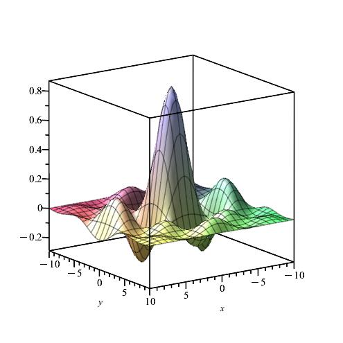
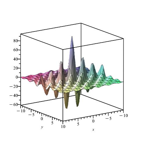
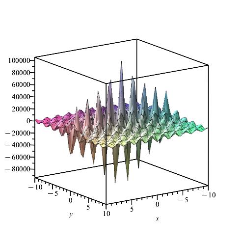
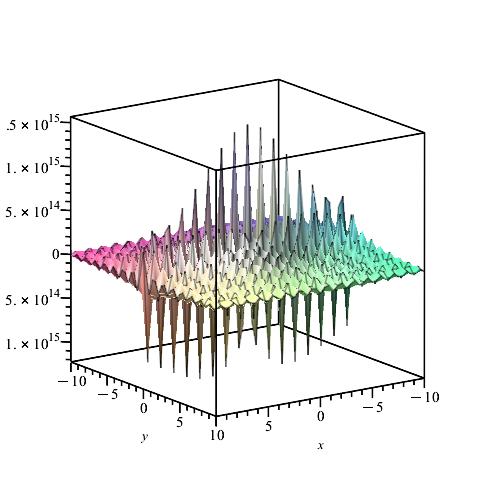
In this section we give numerical applications in the Bessel case and Weinstein case when $\alpha =0$. The first application concerning the solution of Tikhonov problem

$$\underset{f\in {𝒫}_s^B}{inf}\left\{{\Vert h-T_m^B(f)\Vert }_{L^2(\mu )}^2\right\},$$

where $h\in L^2(\mu )$. The solution of this problem will be denoted by $f_{0,h}^{\ast ,B}$. And the second application concerning the solution of the Tikhonov problem

$$\underset{f\in {𝒫}_s^W}{inf}\left\{{\Vert h-T_m^W(f)\Vert }_{L^2({\mu }^{\prime })}^2\right\}.$$

The solution of this problem will be denoted by $f_{0,h}^{\ast ,W}$.

a) The Bessel operator. In this subsection we consider the operator

$${\mathrm{\Delta }}_B:=\frac{{\text{d}}^2}{\text{d}{x}^2}+\frac{1}{x}\frac{\text{d}}{\text{d}x}.$$

In this case $\rho =0$ and ${\phi }_{\lambda }^B(x)=j_0(\lambda x)$, where $j_0$ is the spherical Bessel function of order 0 given by

(10) $$j_0(x)=\frac{1}{\pi }{\int }_0^{\pi }\cos (x\sin t))\text{d}t=\sum {}^{\mathrm{\infty }}{}_{n=0}\frac{{(-1)}^n}{2^{2n}{(n!)}^2}x{}^{2n}.$$

Hence

$${ℱ}_B(h)(\lambda ):={\int }_{{ℝ}_{+}}{j}_0(\lambda x)h(x)x\text{d}x,\lambda \in {ℝ}_{+}.$$

In the following we choose $h(x)=e^{-x^2}$ and $m(\lambda )=e^{-t{\lambda }^2}$, $t>0$. Then

$${ℱ}_B(h)(\lambda )=\frac{1}{2}{e}^{-\frac{{\lambda }^2}{4}}.$$

Therefore, and by Theorem 3 (i) and Theorem 4 (i) we obtain

$$f_{\eta ,h}^{\ast ,B}(y)=\frac{1}{2}{\int }_0^{1/s}\frac{j_0(\lambda y)e^{-\frac{{\lambda }^2}{4}}}{\eta e^{t{\lambda }^2}+e^{-t{\lambda }^2}}\lambda \text{d}\lambda ,$$

and

$$T_m^B(f_{\eta ,h}^{\ast ,B})(y)=\frac{1}{2}{\int }_0^{1/s}\frac{j_0(\lambda y)e^{-\frac{{\lambda }^2}{4}}}{\eta e^{2t{\lambda }^2}+1}\lambda \text{d}\lambda .$$

Next, taking $\eta \to 0^{+}$ yields

$$f_{0,h}^{\ast ,B}(y)=\frac{1}{2}{\int }_0^{1/s}{j}_0(\lambda y)e^{(t-\frac{1}{4}){\lambda }^2}\lambda \text{d}\lambda ,$$

and

$$T_m^B(f_{0,h}^{\ast ,B})(y)=\frac{1}{2}{\int }_0^{1/s}{j}_0(\lambda y)e^{-\frac{{\lambda }^2}{4}}\lambda \text{d}\lambda .$$

From (10) we deduce that

(11) $$f_{0,h}^{\ast ,B}(y)=\frac{1}{2\pi }{\int }_0^{1/s}{\int }_0^{\pi }\lambda \cos (\lambda y\sin \tau )e^{(t-\frac{1}{4}){\lambda }^2}\text{d}\tau \text{d}\lambda ,$$

and

(12) $$T_m^B(f_{0,h}^{\ast ,B})(y)=\frac{1}{2\pi }{\int }_0^{1/s}{\int }_0^{\pi }\lambda \cos (\lambda y\sin \tau )e^{-\frac{{\lambda }^2}{4}}\text{d}\tau \text{d}\lambda .$$

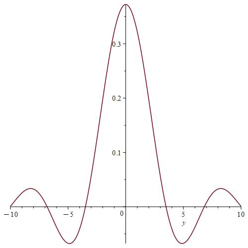
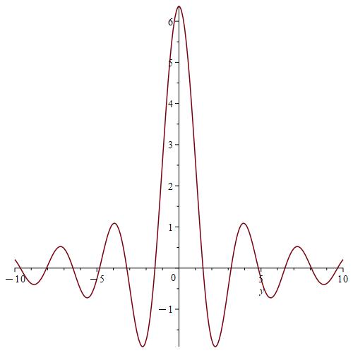
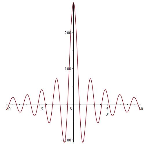
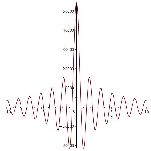
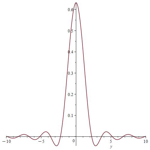
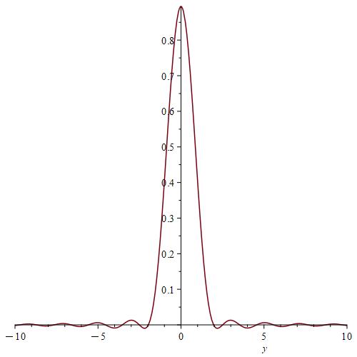
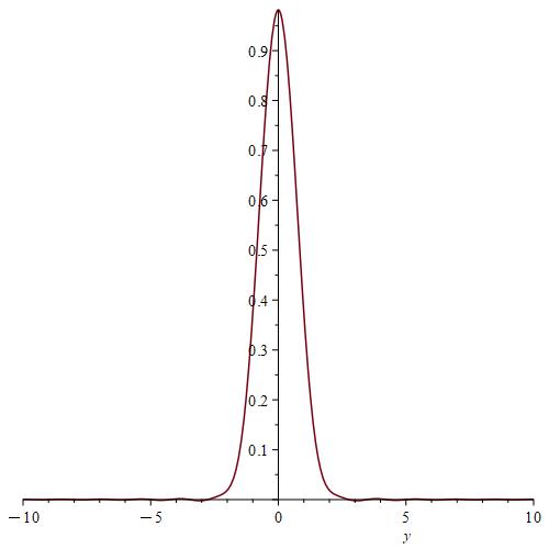
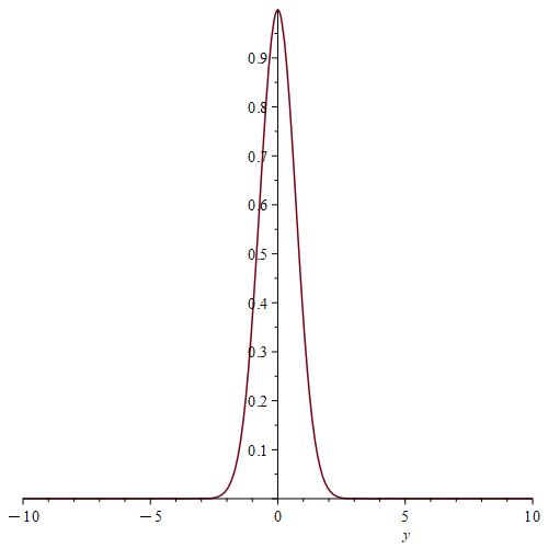
We calculate $f_{0,h}^{\ast ,B}(y)$ and $T_m^B(f_{0,h}^{\ast ,B})(y)$ for $y\in [-10,10]$, by using the Gauss-Kronrod method and Maple.

Figure 1. $s=1$

Figure 2. $s=\frac{1}{2}$

Figure 3. $s=\frac{1}{3}$

Figure 4. $s=\frac{1}{4}$

Figure 5. $s=\frac{1}{5}$

Figure 6. $s=\frac{1}{10}$

In Fig. 6–Fig. 6, we display the plot of $f_{0,h}^{\ast ,B}(y)$ for $y\in [-10,10],t=1$ and $s=1,\frac{1}{2},\frac{1}{3},\frac{1}{4},\frac{1}{5},\frac{1}{10}$.

Figure 7. $s=1$

Figure 8. $s=\frac{1}{2}$

Figure 9. $s=\frac{1}{5}$

Figure 10. $s=\frac{1}{7}$

Figure 11. $s=\frac{1}{50}$

Figure 12. $s=\frac{1}{100}$

In Fig. 12–Fig. 12, we display the plot of $f_{0,h}^{\ast ,B}(y)$ for $y\in [-10,10]$, $t={10}^{-7}$ and $s=1,\frac{1}{2},\frac{1}{5},\frac{1}{7},\frac{1}{50},\frac{1}{100}$.

Figure 13. $s=1$

Figure 14. $s=\frac{1}{2}$

Figure 15. $s=\frac{1}{5}$

Figure 16. $s=\frac{1}{10}$

Figure 17. $s=\frac{1}{50}$

Figure 18. $s=\frac{1}{100}$

In Fig. 18–Fig. 18, we display the plot of $T_m^B(f_{0,h}^{\ast ,B})(y)$ for $y\in [-10,10]$ and $s=1,\frac{1}{2},\frac{1}{5},\frac{1}{10},\frac{1}{50},\frac{1}{100}$.

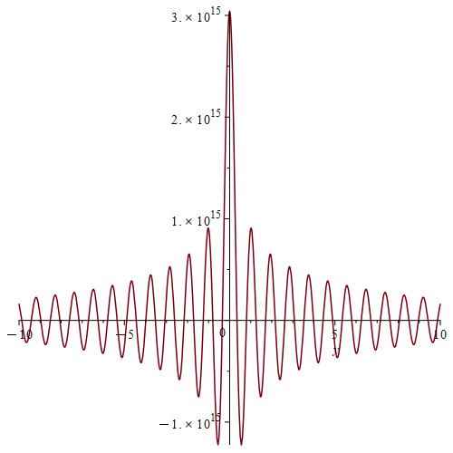
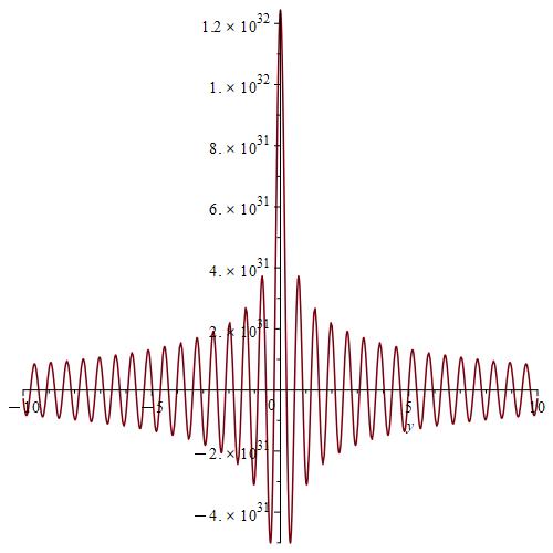
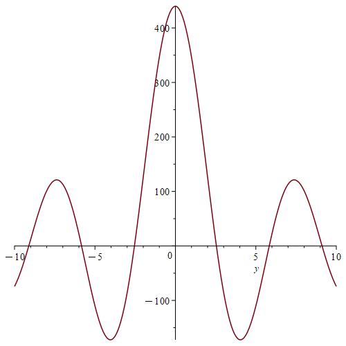
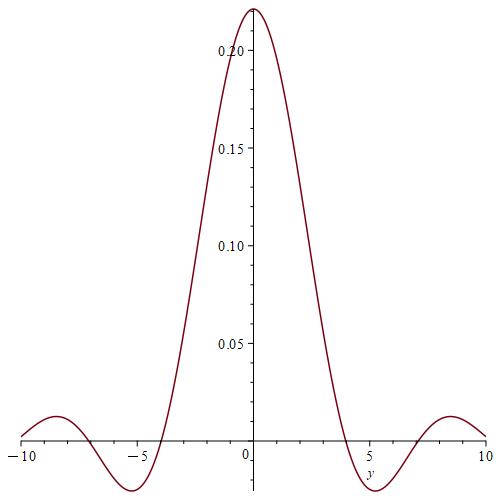
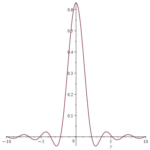
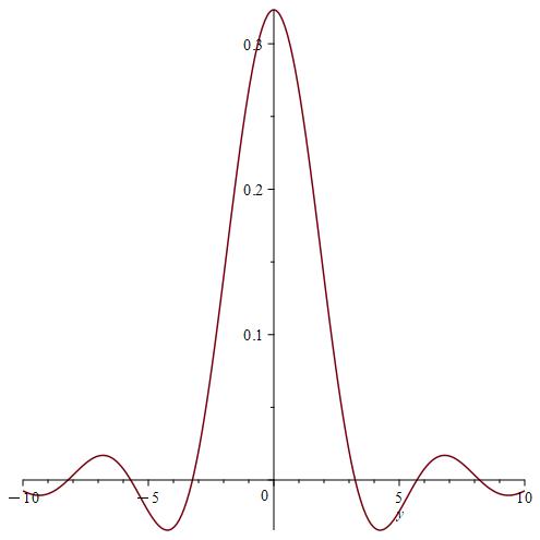
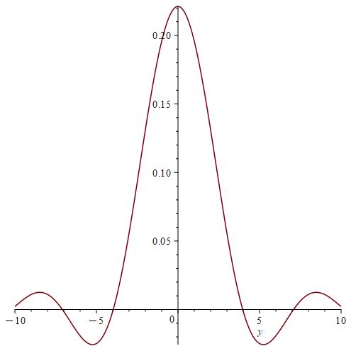
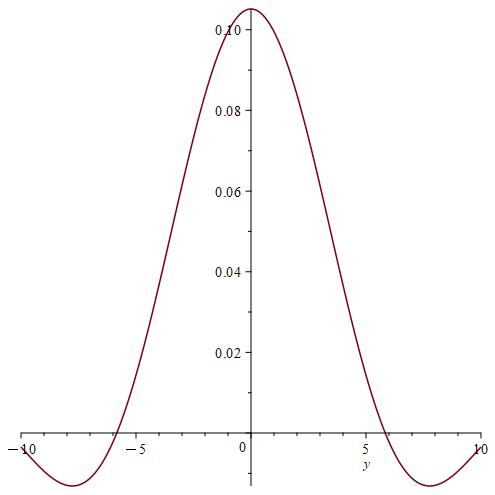
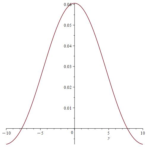
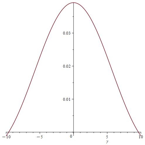
Remark 7.

We notice from Fig. 6–Fig. 6 that for a small value of $s$ and when $t$ is fixed at 1, the stability of the function $f_{0,h}^{\ast ,B}(y)$ is reached. However, when $t$ approaches 0 (Fig. 12–Fig. 12), the stability of $f_{0,h}^{\ast ,B}(y)$ is quickly reached and its maximum is maintained over a specific range of $s$. Fig. 18–Fig. 18 show that the desired approximate formulas can be obtained in practice. However, Theorem 4 is justified; we were able to numerically realize the limiting case $\eta \to 0^{+}$ using computers.

b) The Weinstein operator. In this subsection we consider the operator

$${\mathrm{\Delta }}_W:=\frac{{\text{d}}^2}{\text{d}{x}_1^2}+\frac{{\text{d}}^2}{\text{d}{x}_2^2}+\frac{1}{x_2}\frac{\text{d}}{\text{d}{x}_2}.$$

In this case $\rho =0$ and ${\phi }_{{\lambda }_1,{\lambda }_2}^W(x_1,x_2)=e^{-i{\lambda }_1{x}_1}{j}_0({\lambda }_2{x}_2)$. Hence

$${ℱ}_W(h)({\lambda }_1,{\lambda }_2):={\int }_{𝕂}{e}^{-i{\lambda }_1{x}_1}{j}_0({\lambda }_2{x}_2)h(x_1,x_2)x_2\text{d}{x}_1\text{d}{x}_2,({\lambda }_1,{\lambda }_2)\in 𝕂.$$

In the following we choose $h(x_1,x_2)=e^{-(x_1^2+x_2^2)}$ and $m({\lambda }_1,{\lambda }_2)=e^{-t({\lambda }_1^2+{\lambda }_2^2)}$, $t>0$. Then

$${ℱ}_W(h)({\lambda }_1,{\lambda }_2)=\frac{\sqrt{\pi }}{2}{e}^{-\frac{1}{4}({\lambda }_1^2+{\lambda }_2^2)}.$$

Therefore, and by Theorem 6 (i) and (ii) we obtain

$$f_{\eta ,h}^{\ast ,W}(y_1,y_2)=\frac{1}{4\sqrt{\pi }}{\int }_{-1/s}^{1/s}{\int }_0^{1/s}\frac{e^{-i{\lambda }_1{y}_1}{j}_0({\lambda }_2{y}_2)e^{-\frac{1}{4}({\lambda }_1^2+{\lambda }_2^2)}}{\eta e^{t({\lambda }_1^2+{\lambda }_2^2)}+e^{-t({\lambda }_1^2+{\lambda }_2^2)}}{\lambda }_2\text{d}{\lambda }_1\text{d}{\lambda }_2,$$

and

$$T_m^W(f_{\eta ,h}^{\ast ,W})(y_1,y_2))=\frac{1}{4\sqrt{\pi }}\int {}^{1/s}{}_{-1/s}\int {}^{1/s}{}_0\frac{e^{-i{\lambda }_1{y}_1}{j}_0({\lambda }_2{y}_2)e^{-\frac{1}{4}({\lambda }_1^2+{\lambda }_2^2)}}{\eta e^{2t({\lambda }_1^2+{\lambda }_2^2)}+1}\lambda {}_2\text{d}\lambda {}_1\text{d}\lambda {}_2.$$

Next, taking $\eta \to 0^{+}$ yields

$f_{0,h}^{\ast ,W}(y_1,y_2)$ $=$ $\frac{1}{4\sqrt{\pi }}{\displaystyle {\int }_{-1/s}^{1/s}}{\displaystyle {\int }_0^{1/s}}{e}^{-i{\lambda }_1{y}_1}{j}_0({\lambda }_2{y}_2)e^{(t-\frac{1}{4})({\lambda }_1^2+{\lambda }_2^2)}{\lambda }_2\text{d}{\lambda }_1\text{d}{\lambda }_2$

$=$ $f_{0,h}^{\ast ,1}(y_1).f_{0,h}^{\ast ,2}(y_2),$

where

$$f_{0,h}^{\ast ,1}(y_1)=\frac{1}{2\sqrt{\pi }}{\int }_{-1/s}^{1/s}{e}^{-i{\lambda }_1{y}_1}{e}^{(t-\frac{1}{4}){\lambda }_1^2}\text{d}{\lambda }_1$$

and

$$f_{0,h}^{\ast ,2}(y_2)=\frac{1}{2}{\int }_0^{1/s}{j}_0({\lambda }_2{y}_2)e^{(t-\frac{1}{4}){\lambda }_2^2}{\lambda }_2\text{d}{\lambda }_2.$$

Furthermore

$T_m^W(f_{0,h}^{\ast ,W})(y_1,y_2)$ $=$ $\frac{1}{4\sqrt{\pi }}{\displaystyle {\int }_{-1/s}^{1/s}}{\displaystyle {\int }_0^{1/s}}{e}^{-i{\lambda }_1{y}_1}{j}_0({\lambda }_2{y}_2)e^{-\frac{1}{4}({\lambda }_1^2+{\lambda }_2^2)}{\lambda }_2\text{d}{\lambda }_1\text{d}{\lambda }_2$

$=$ $T_m^W{f}_{0,h}^{\ast ,1}(y_1).T_m^W{f}_{0,h}^{\ast ,2}(y_2),$

where

$$T_m^W(f_{0,h}^{\ast ,1})(y_1)=\frac{1}{2\sqrt{\pi }}{\int }_{-1/s}^{1/s}{e}^{-i{\lambda }_1{y}_1}{e}^{-\frac{1}{4}{\lambda }_1^2}\text{d}{\lambda }_1$$

and

$$T_m^W(f_{0,h}^{\ast ,2})(y_2)=\frac{1}{2}{\int }_0^{1/s}{j}_0({\lambda }_2{y}_2)e^{-\frac{1}{4}{\lambda }_2^2}{\lambda }_2\text{d}{\lambda }_2.$$

From (11) and (12) we deduce that

$$f_{0,h}^{\ast ,2}(y_2)=\frac{1}{2\pi }{\int }_0^{1/s}{\int }_0^{\pi }\lambda \cos ({\lambda }_2{y}_2\sin \tau )e^{(t-\frac{1}{4}){\lambda }_2^2}\text{d}\tau \text{d}{\lambda }_2,$$

and

$$T_m^W(f_{0,h}^{\ast ,2})(y_2)=\frac{1}{2\pi }{\int }_0^{1/s}{\int }_0^{\pi }{\lambda }_2\cos ({\lambda }_2{y}_2\sin \tau )e^{-\frac{{\lambda }_2^2}{4}}\text{d}\tau \text{d}{\lambda }_2.$$

We calculate $f_{0,h}^{\ast ,W}(y_1,y_2)$ and $T_m^W{f}_{0,h}^{\ast ,W}(y_1,y_2)$ for $(y_1,y_2)\in [-10,10]\times [0,10]$, by using the Gauss-Kronrod method and Maple.

Figure 19. $s=1$

Figure 20. $s=\frac{1}{2}$

Figure 21. $s=\frac{1}{3}$

Figure 22. $s=\frac{1}{4}$

Figure 23. $s=\frac{1}{5}$

Figure 24. $s=\frac{1}{10}$

In Fig. 24–Fig. 24, we display the plot of $f_{0,h}^{\ast ,W}(y_1,y_2)$ for $(y_1,y_2)\in [-10,10]\times [0,10]$, $t=1$ and $s=1,\frac{1}{2},\frac{1}{3},\frac{1}{4},\frac{1}{5},\frac{1}{10}$.

Figure 25. $s=1$

Figure 26. $s=\frac{1}{2}$

Figure 27. $s=\frac{1}{3}$

Figure 28. $s=\frac{1}{10}$

Figure 29. $s=\frac{1}{50}$

Figure 30. $s=\frac{1}{100}$

In Fig. 30–Fig. 30, we display the plot of $T_m^W(f_{0,h}^{\ast ,W})(y_1,y_2)$ for $(y_1,y_2)\in [-10,10]\times [0,10]$ and $s=1,\frac{1}{2},\frac{1}{3},\frac{1}{10},\frac{1}{50},\frac{1}{100}$.

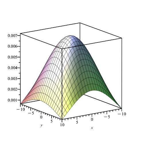
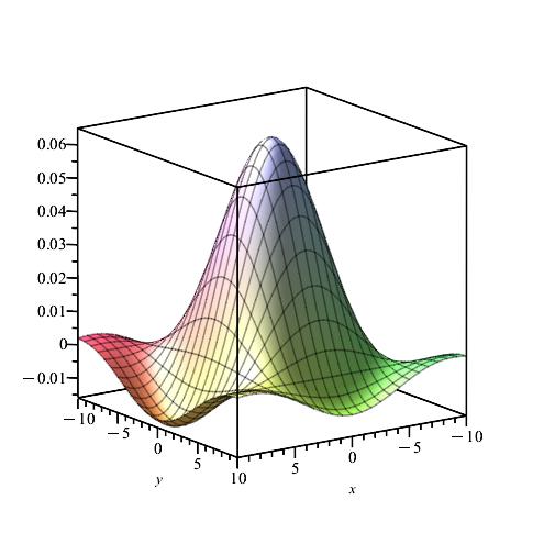
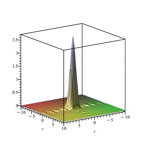
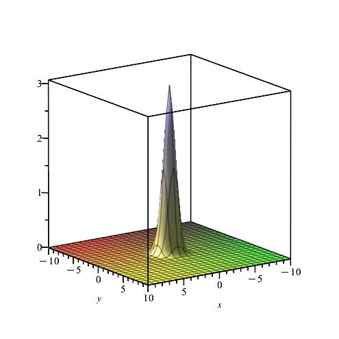
Remark 8.

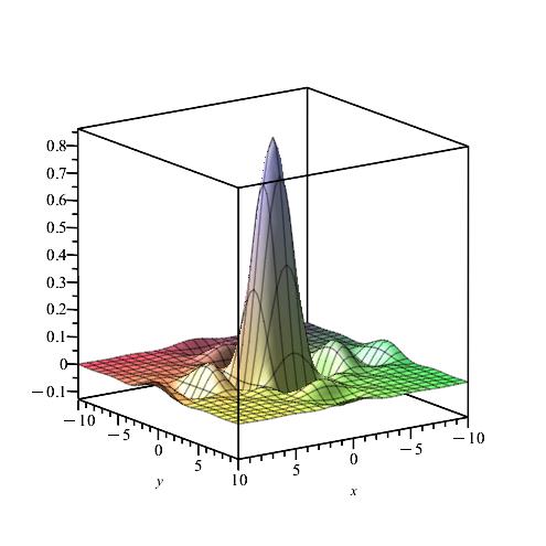
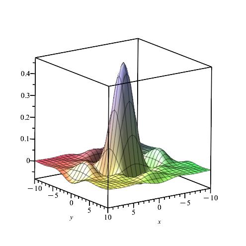
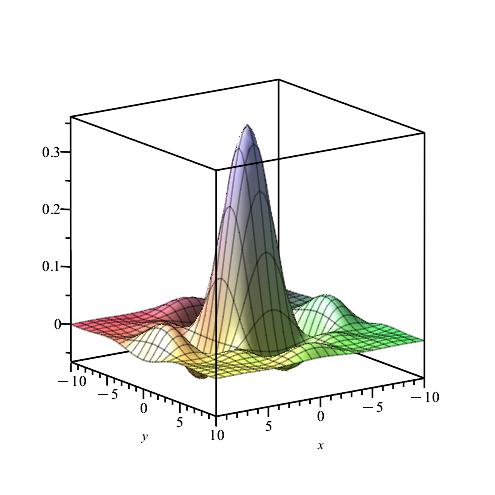
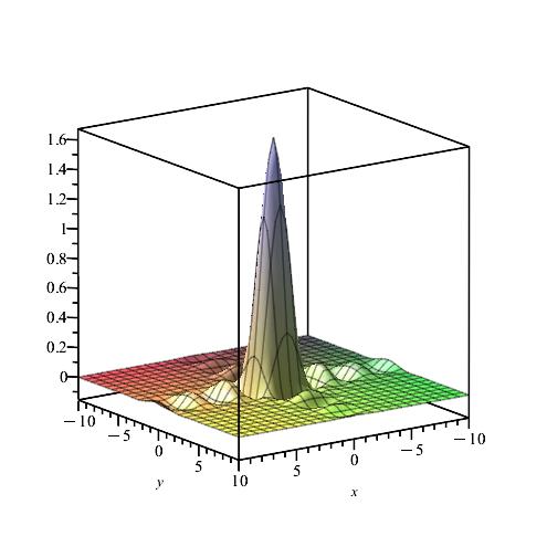
We notice from Figures Fig. 24–Fig. 24 that for a small value of $s$ and when $t$ is fixed at 1, the stability of the function $f_{0,h}^{\ast ,W}(y_1,y_2)$ is reached. Fig. 30–Fig. 30 show that the desired approximate formulas can be obtained in practice. However, Theorem 6 is justified; we were able to numerically realize the limiting case $\eta \to 0^{+}$ using computers.

Acknowledgements.

The authors are deeply grateful to the referees for their constructive comments and valuable suggestions.