Modified adaptive quadrature by expansion
for Laplace and Helmholtz layer potentials in 2D^∗

Abstract.

An adaptive algorithm based on quadrature by expansion (QBX) is proposed for computing layer potentials at target points near or on a smooth boundary in ${ℝ}^2$. The algorithm can be viewed as a major modification to the two-phase algorithm AQBX, proposed recently by Klinteberg et al. [SIAM Journal on Scientific Computing, 40(3), 2018]. In the modified AQBX (MAQBX), we consider sharper bounds for the involved truncation error. As a result, the involved stopping criteria are met earlier, and the total computational cost is reduced. Moreover, MAQBX is a single-phase algorithm and its structure is far simpler than that of AQBX. It is recommended that QBX (or any version of it) should be applied on a small part of the boundary that is near the target point, and a classical quadrature is applied on the rest of the boundary (this is often referred to as local QBX). We partially show that for Laplace and Helmholtz potentials, parametric symmetry of the target point with respect to the near part, can improve the convergence of QBX. Based on this observation, we suggest the local MAQBX that is very efficient in practice both for computing layer potentials and for solving boundary integral equations via the Nyström scheme.

In boundary integral methods (BIMs), one uses Green theorems and transform a boundary value problem (BVP) for PDEs to a well-posed integral equation on the boundary of the domain of definition of the problem (note that the domain of application of BIMs extends far beyond the scope of PDEs). This has many advantages over the traditional volume PDE solvers such as FD, FEM, etc: 1) the dimension of the problem is reduced by one, so one needs fewer sample points to achieve a given accuracy, 2) an exterior problem with an unbounded spatial domain is reduced to a boundary integral equation over a bounded domain, 3) solving integral equations of the second kind is more numerically stable than solving PDEs directly by traditional discretization methods, 4) through the Nyström method, the problem of solving an integral equations of the second kind is reduced to the simpler problem of numerical quadrature or cubature for which high-order rules exist, 5) moving boundaries can be handled more easily, 6) a boundary integral formulation reflects well-posedness of the underlying physical problem more fairly, etc.

Assume that $G$ is the fundamental solution of the PDE associated with a BVP defined in a domain $\mathrm{\Omega }\subset {ℝ}^d$, $d\ge 1$. In a BIM, the solution $u$ of the problem is represented as a layer potential with a jump discontinuity on the boundary $\partial \mathrm{\Omega }$. This jump discontinuity is essential in well-posedness of the resulting boundary integral equation. Consider the double layer potential

(1) $$D\sigma (x):={\int }_{\partial \mathrm{\Omega }}\frac{\partial G}{\partial n_{x^{\prime }}}(x,x^{\prime })\sigma (x^{\prime })d{x}^{\prime },$$

(with $n_{x^{\prime }}$ the outer unit normal at $x^{\prime }$) and the single layer potential

(2) $$S\sigma (x):={\int }_{\partial \mathrm{\Omega }}G(x,x^{\prime })\sigma (x^{\prime })d{x}^{\prime }.$$

The double layer potential itself and the gradient of the single layer potential satisfy jump discontinuity properties. Thus, the double layer and the single layer potentials are suitable for Dirichlet and Neumann problems, respectively. For the sake of solvability, one usually uses a combined field representation

(3) $$u(x)=(D+\alpha S)\sigma (x),x\in \mathrm{\Omega },$$

where $\alpha \ne 0$ is a coupling parameter. For a Dirichlet problem with the Dirichlet data $f$ on the boundary, we obtain the following boundary integral equation for the unknown density function $\sigma$:

(4) $$\left(\pm \frac{1}{2}I+D+\alpha S\right)\sigma (x)=f(x),x\in \partial \mathrm{\Omega },$$

where the positive and the negative signs correspond to the exterior and the interior problem, respectively. If $\tilde{\sigma }$ is an approximate solution of (4), the solution to BVP at the target point $x$ is achieved by computing the layer potential $(D+\alpha S)\tilde{\sigma }(x)$. For Neumann and Robin boundary conditions, BIM is also led to integral equations of the second kind, which are known to be well-posed (see [11] and references therein).

In this paper, we focus on two-dimensional Laplace and Helmholtz problems, though the theory is readily applicable to other problems.

In BIM, singularity is a price which should be paid for well-posedness. Indeed, the singularity of the fundamental solution yields the jump discontinuity property of the layer potential, and the latter causes the term $\pm I/2$ in (4), which renders the boundary integral equation to a well-posed integral equation of the second kind. Singularity of the fundamental solution is inherited by both the boundary integral equation and the layer potential. Indeed, the boundary integral equation is weakly singular, and the layer potential at a target point near the boundary is a nearly singular integral. There are several efficient numerical methods for both the problems (see e.g., [5, 7, 8, 9, 10, 13, 14, 15, 16, 18, 22]), but there is still the need to design more robust algorithms.

Quadrature by expansion (QBX) was introduced in [17] for computing layer potentials at target points on or near the boundary. QBX is easy to implement, high order accurate, and despite earlier methods, dimension-independent. Moreover, QBX can be coupled with fast multipole methods (FMMs) and introduce fast algorithms for both the problems of solving boundary integral equations and computing layer potentials at target points near the boundary. In QBX, the singular integrand is locally expanded about a center with a suitable distance from the boundary. As a result, the singular or nearly singular layer potential is approximated by a sum of several regular integrals. Due to its individual benefits, QBX has been the subject of many studies for the last decade. In [6, 12, 3], convergence of QBX is studied in depth. Some combinations of QBX with FMM are suggested in [26, 25, 20]. QBX has also found applications in simulating spheroids in periodic Stokes flow [2]. For other applications and modifications of QBX one can see [4, 21, 23, 27].

One of the difficulties of QBX is the choice of parameters to achieve the optimal accuracy. The distance $r$ of the expansion center from the boundary, the order $p$ of the expansion, and the number $N$ of abscissas for the underlying quadrature have unspecific interactions on the total accuracy. For example, when $p$ grows, the total error can decreases or increases depending on the values of $r$ and $N$. Thus, there is an urgent need to determine optimal parameters to achieve a given accuracy.

In [4], this problem has been studied in depth, and an adaptive algorithm is proposed for determining $p$ and $N$, for a given $r$. In adaptive QBX, the potential is written as the inner product of a vector of coefficients involving regular integrals over the boundary and a vector of norm one. The error in QBX can be separated into a truncation error and a coefficient error. In adaptive QBX, practical a priori estimates for both of the errors are suggested, which enable one to determine the optimal parameters in order to achieve a given accuracy. The algorithm has two phases. In the first phase, the coefficients are computed by the Gauss-Legendre rules to a given accuracy. In the core of this phase, there is a usable and sharp a priori error estimate for the Gauss-Legendre quadrature. The idea is developed by contour integrals and residue calculus, which was extended later to curves and surfaces in ${ℝ}^3$ [1, 24]. Meanwhile, the coefficients are computed till a stopping criterion is met for the truncation error. In the second phase, the potential is computed by considering a different stopping criterion for the truncation error. Indeed, in the first phase, an upper bound is employed for the truncation error to compute coefficients contributing in the second phase, while in the second phase, a sharper bound is used to evaluate the potential. This causes that some coefficients are computed in the first phase that do not have any contribution in the second phase, and this in turn exposes an extra and unnecessary computational cost.

In the present paper, we address the above issue. If we consider the sharper bound in both the phases, then they merge into a single one, resulting a modified algorithm that is simpler as well as faster in practice. We also propose some other modifications which improve the logic and convergence of adaptive QBX. The estimate suggested in [4] for the coefficient error actually depends on $p$. Here, we suggest a $p$-independent one, which gives a more reasonable bound for the coefficient error. Also, we partially show that for Laplace and Helmholtz potentials, if some symmetry conditions are hold, the convergence of QBX is improved. Such conditions can easily be hold without imposing an extra computational cost.

The rest of paper is organized as follows. In  Section 1, a brief review of QBX is given.  Section 2 contains the modifications to the AQBX algorithm of [4], based on which, we devise the modified AQBX (MAQBX) algorithm in  Section 3. We carry out some numerical experiments in  Section 4 to illustrate the efficiency of the MAQBX algorithm for computing layer potentials as well as solving boundary integral equations. Finally, we give some conclusions in  Section 5.

1. QBX

In this section, we give a review of QBX and its localization. Assume that $\mathrm{\Omega }\subset {ℝ}^2$ is either interior or exterior of a bounded domain in ${ℝ}^2$ with smooth boundary $\partial \mathrm{\Omega }$. In 2D, it is more convenient to consider ${ℝ}^2$ as the complex plain $ℂ$ and write the potentials in the complex setting. Assume that $\gamma$ is an analytic $2\pi$-periodic counterclockwise parametrization of the boundary, that is $\gamma ([0,2\pi ])=\partial \mathrm{\Omega }$. Assume also that the boundary is so smooth that ${\gamma }^{\prime }$ never vanishes. Then, the outer normal $n(t)$ at any point $t\in [0,2\pi )$, is determined by $-\mathrm{i}{\gamma }^{\prime }(t)/|{\gamma }^{\prime }(t)|$.

In the complex setting, a 2D layer potential can be written in form of

(5) $$u(z)={\int }_{\partial \mathrm{\Omega }}K(z,w)\sigma (w)d{s}_w,$$

where $z$ is the target point in ${ℝ}^2$, $K$ is a linear combination of the fundamental solution and its normal derivative, and $\mathrm{d}{s}_w$ is the arc length element with respect to $w$.

The main assumption of QBX is that the variables of $K$ can be separated by a known addition theorem as

(6)

where $A_m^r$ and $B_m^r$ are either scalars or 2-vectors with given $r$, the distance of the expansion center $z_0$ from the boundary. Note that $K(w,w)$ is unbounded for any $w\in \partial \mathrm{\Omega }$, thus the expansion (6) should have a singular factor. We assume that $B_m^r$ is bounded and $A_m^r$ is the singular part, i.e., $A_m^r(w,w)$ is unbounded for any $w\in \partial \mathrm{\Omega }$. We also assume that (6) is normalized as

(7) $\left|B_m^r(z,z_0)\right|\le 1,$

(8) $\underset{m,z}{\max }\left|B_m^r(z,z_0)\right|=1,$

for $|z-z_0|\le r$ and integer $m\ge 0$. This normalization is necessary in adaptive QBX (see [4]).

From (6), the potential (5) can be written as

(9) $$u(z)=\sum _{m=0}^{\mathrm{\infty }}{a}_m{B}_m^r(z,z_0),$$

where

(10) $$a_m:={\int }_{\partial \mathrm{\Omega }}{A}_m^r(w,z_0)\sigma (w)d{s}_w.$$

Since the expansion center is far away from the boundary, the integrals (10) are regular and can be approximated by classical quadrature rules to the given accuracy. Assume that $a_m$, for each $m$, is approximated by ${\tilde{a}}_m$. When the distance of $z$ from the boundary is less than $r$, the $u(z)$ can be approximated by QBX as

(11) $$u_p(z):=\sum _{m=0}^p{\tilde{a}}_m{B}_m^r(z,z_0).$$

The total error is the summation of the truncation error ($e_{\mathrm{T}}$) and the coefficient error ($e_{\mathrm{C}}$):

(12) $$u(z)-u_p(z)=\underset{e_{\mathrm{T}}}{\underbrace{u(z)-\sum _{m=0}^p{a}_m{B}_m^r(z,z_0)}}+\underset{e_{\mathrm{C}}}{\underbrace{\sum _{m=0}^p(a_m-{\tilde{a}}_m)B_m^r(z,z_0)}}.$$

See [12] for an error analysis. In practice, the truncation error decreases almost exponentially as $r^p$ when $p$ grows. The coefficient error depends on the accuracy of the underlying quadrature rule, but it can be deteriorated as $p$ increases. The interplay between $e_{\mathrm{T}}$ and $e_{\mathrm{C}}$, as $p$ grows, naturally leads us to search for the optimal $p$, which minimizes the total error.

The paper [4] was the first attempt to study this problem in depth, and here, we give some revisions to the algorithm proposed in [4]. Before that, we complete this section by determining $A_m^r$ and $B_m^r$ for Laplace and Helmholtz layer potentials.

1.1. Laplace double layer potential

Fundamental solution of the 2D Laplace problem is $\mathrm{\Phi }(x,x^{\prime })=-\log |x-x^{\prime }|/(2\pi )$. In the complex setting, the corresponding double layer potential can be written as $u=\mathrm{\Re }v$, where

(13) $$v(z)=\frac{1}{2\pi }{\int }_{\partial \mathrm{\Omega }}\frac{n_w}{z-w}\sigma (w)d{s}_w,z\in ℂ\setminus \partial \mathrm{\Omega }.$$

Now, from the Taylor expansion

(14)

the corresponding $A_m^r$ and $B_m^r$ is specified

(15a) $A_m^r(y,z_0)$ $=-\frac{r^m{n}_w}{2\pi {(w-z_0)}^{m+1}},$

(15b) $B_m^r(z,z_0)$ $=\frac{{(z-z_0)}^m}{r^m}.$

1.2. Laplace single layer potential

In the complex setting, the Laplace single layer potential can be written as $u=\mathrm{\Re }v$, where

(16) $$v(z)=\frac{1}{2\pi }{\int }_{\partial \mathrm{\Omega }}\log \left(\frac{1}{w-z}\right)\sigma (w)d{s}_w,z\in ℂ\setminus \partial \mathrm{\Omega }.$$

Now, from the Taylor expansion

$\log \left(\frac{1}{w-z}\right)$ $=\log \left(\frac{1}{w-z_0}\right)-\log \left(1-\frac{z-z_0}{w-z_0}\right)$

(17)

the corresponding $A_m^r$ and $B_m^r$ is specified by

(18a) $A_0^r(w,z_0)$ $=\frac{1}{2\pi }\log \left(\frac{1}{w-z_0}\right),$

(18b) $A_m^r(w,z_0)$ $=\frac{1}{2\pi m}\frac{r^m}{{(w-z_0)}^{m+1}},m>0,$

(18c) $B_m^r(z,z_0)$ $=\frac{{(z-z_0)}^m}{r^m},m=0,1,\mathrm{\dots }.$

1.3. Helmholtz double layer potential

In the complex setting, fundamental solution of the 2D Helmholtz problem with the wave number $k$ is

(19) $${\mathrm{\Phi }}_k(z,w)=\frac{\mathrm{i}}{4}{H}_0^{(1)}(k|z-w|).$$

For Helmholtz potentials, one uses the Graf addition theorem [19, §10.23(ii)],

(20)

where $(r_w,{\theta }_w)$ and $(r_z,{\theta }_z)$ are polar coordinates of $w-z_0$ and $z-z_0$, respectively, i.e.,

(21a) $r_w$ $=|w-z_0|,$

(21b) ${\mathrm{e}}^{\mathrm{i}{\theta }_w}$ $=\frac{w-z_0}{|w-z_0|},$

(21c) $r_z$ $=|z-z_0|,$

(21d) ${\mathrm{e}}^{\mathrm{i}{\theta }_z}$ $=\frac{z-z_0}{|z-z_0|}.$

Then, the corresponding $A_m^r$ and $B_m^r$ are given as follows (see [4])

(22a) $A_0^r(w,z_0)$ $=d_0(w,z_0)$

(22b) $B_0^r(z,z_0)$ $=J_0(k{r}_z)$

(22c) $A_m^r(w,z_0)$ $={\alpha }_m^r(d_m(w,z_0),d_{-m}(w,z_0)),m>0,$

(22d) $B_m^r(z,z_0)$ $=\frac{1}{{\alpha }_m^r}(J_m(k{r}_z){\mathrm{e}}^{\mathrm{i}m{\theta }_z},J_{-m}(k{r}_z){\mathrm{e}}^{-\mathrm{i}m{\theta }_z}),m>0,$

where

(23) $${\alpha }_m^r:=\frac{\sqrt{2}}{m!}{\left(\frac{kr}{2}\right)}^m,m>0,$$

and

(24) $$d_m(w,z_0)=\frac{\mathrm{i}k}{8}\left(H_{m-1}^{(1)}(k{r}_w){\mathrm{e}}^{-\mathrm{i}(m-1){\theta }_w}{\overline{n}}_w-H_{m+1}^{(1)}(k{r}_w){\mathrm{e}}^{-\mathrm{i}(m+1){\theta }_w}{n}_w\right),$$

for all $m\ge 0$. Note that $A_m^r$ and $B_m^r$ are 2-vectors for $m>0$

1.4. Helmholtz single layer potential

Again, the Graf addition theorem implies that $A_m^r$ and $B_m^r$, corresponding to the Helmholtz single layer potential, are as follows (see [4])

(25a) $A_0^r(w,z_0)$ $=s_0(w,z_0)$

(25b) $B_0^r(z,z_0)$ $=J_0(k{r}_z)$

(25c) $A_m^r(w,z_0)$ $={\alpha }_m^r(s_m(w,z_0),s_{-m}(w,z_0)),m>0,$

(25d) $B_m^r(z,z_0)$ $=\frac{1}{{\alpha }_m^r}(J_m(k{r}_z){\mathrm{e}}^{\mathrm{i}m{\theta }_z},J_{-m}(k{r}_z){\mathrm{e}}^{-\mathrm{i}m{\theta }_z}),m>0,$

where ${\alpha }_m^r$ are defined by (23), and

(26) $$s_m(w,z_0)=\frac{\mathrm{i}}{4}{H}_m^{(1)}(k{r}_w){\mathrm{e}}^{-\mathrm{i}m{\theta }_w},$$

for all $m\ge 0$.

1.5. Localization

For integration of (5), one can split the integration path as $\partial \mathrm{\Omega }={\mathrm{\Gamma }}^{\mathrm{near}}\cup {\mathrm{\Gamma }}^{\mathrm{far}}$ into the ‘near part’ and the ‘far part’. The near part contains points of the boundary which are so near the target point $z$, that classical quadrature rules on ${\mathrm{\Gamma }}^{\mathrm{near}}$ with a moderate number of abscissas leads to rather large error. More precisely, for a given integer $\mathrm{\ell }\in [0,1)$,

(27) $${\mathrm{\Gamma }}^{\mathrm{near}}=\{w\in \partial \mathrm{\Omega }:|w-z|\le \mathrm{\ell }r\}.$$

Discussion on the choice of $\mathrm{\ell }$ is beyond the scope of this article; interested reader can refer [6, 4] for some comments.

It is recommended that QBX is used only on the near part, and a traditional fast quadrature rule is employed for the far part [6, 4]. This is the so-called local QBX that is compatible with FMM. In local QBX, one divides the boundary into smaller pairwise disjoints panels,

(28) $$\partial \mathrm{\Omega }=\bigcup _i{\mathrm{\Gamma }}_i,$$

such that the boundary is well-resolved by the panels, i.e., the curvature of each panel is rather small. One often uses panels of equal length though panels of different lengths are also allowed. In the latter case, it is recommended that the lengths of any two adjacent panels have a ratio in the interval $[1/2,2]$ (see [20] for more details).

Figure 1. The near (red) and the far (green) parts of a boundary with respect to a target point (black asterisk). $z_0^{(j)}$ is the exapnsion center corresponding to the panel ${\mathrm{\Gamma }}_j$, for $j=1,2$.

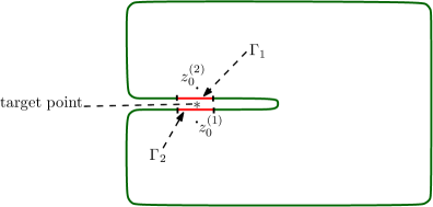
Note that the near (or far) part of a boundary with respect to a target point is not necessarily connected. In Fig. 1, the near part is the union of two disjoint curves ${\mathrm{\Gamma }}_1$ and ${\mathrm{\Gamma }}_2$. QBX is applied for each panel separately with an individual expansion center, i.e., $z_0^{(j)}$ for the panel ${\mathrm{\Gamma }}_j$, for $j=1,2$. Without losing any generality, we assume that the near part is always connected throughout this paper.

In adaptive local QBX, the only input parameter is the error tolerance $\epsilon$. In Section 3, we suggest how to choose $r$ and determine the near part by $\epsilon$. Throughout the paper, by adaptive QBX, we mean adaptive local QBX, and the idea is described on a typical small panel $\mathrm{\Gamma }\subset \partial \mathrm{\Omega }$ that is near to the target point $z$ and in front of it, i.e., the set $\{|z-w|:w\in \mathrm{\Gamma }\}$ takes its minimum at a point in $\mathrm{int}(\mathrm{\Gamma }):=\{w\in \mathrm{\Gamma }:B_{r_w}(w)\cap \partial \mathrm{\Omega }\subseteq \mathrm{\Gamma }\text{ for some }{r}_w>0\}$. Here, $B_{r_w}(w)$ is an open ball of radius $r_w$ centered at $w$.

2. Some improvements in adaptive QBX

In this section, we give some modifications to the two-phase algorithm proposed in [4] for adaptive QBX. In Section 2.1, the first phase, i.e., the coefficient error, is affected by considering more suitable criteria for the coefficient refinement. In Section 2.2 and Section 2.3, we modify the second phase such that the truncation error reaches the stopping threshold more rapidly. In total, one obtains a single-phase algorithm for adaptive QBX (ref.  Section 3) that is simpler and faster than that of [4].

2.1. $p$-independent coefficient error estimate

In the algorithm proposed in [4], the quadrature rule is refined so that for each $m$, where $\epsilon >0$ is a given tolerance. This strategy has this disadvantage that the upper bound for the coefficient error grows linearly with $p$. Indeed,

(29) $$|e_{\mathrm{C}}|\le \sum _{m=0}^p|a_m-{\tilde{a}}_m|\le (p+1)\epsilon .$$

If we use the condition for each $m$ instead, then we gain two advantages. Firstly, ${\tilde{a}}_m$ approximates $a_m$ more accurately since it is assumed that $a_m$ decays exponentially by $m$. Secondly,

(30)

Thus, the upper bound (30) is independent of $p$.

Note that $2^{-m-2}\epsilon$ may reach the machine epsilon ${\epsilon }_{\mathrm{mach}}$ rapidly as $m$ grows. In order to avoid extra effort, one can consider the condition instead. Since one does not expect that $p$ exceeds, e.g. 50, the inequality (30) will still be valid up to a tolerance scalable to the machine precision.

In order to approximate $a_m$ to a given accuracy, we suggest the Gauss-Legendre rules, though any other quadrature rule can also be employed, provided that there exists a practical error bound for it that contains no unknown coefficients and can efficiently be evaluated. In [4], the authors suggest such an a priori estimate $E_{\mathrm{C}}(n,m)$ of $|a_m-{\tilde{a}}_m|$, where ${\tilde{a}}_m$ is an approximation of $a_m$ obtained by the $n$-point Gauss-Legendre quadrature rule:

(31) $$E_{\mathrm{C}}(n,m)=\frac{r^m}{m!}{\left|\frac{2n+1}{{\gamma }^{\prime }(w_0)\sqrt{w_0^2-1}}\right|}^m\frac{|\sigma (w_0)|}{{\left|w_0\pm \sqrt{w_0^2-1}\right|}^{2n+1}},$$

where $\gamma :[-1,1]\to \mathrm{\Gamma }$ is a parametrization of $\mathrm{\Gamma }$, and $w_0$ is a zero of the complex function $w\mapsto \gamma (w)-z_0$. For details on how to approximate $w_0$ and evaluate $E_{\mathrm{C}}(n,m)$ robustly, one can see [4, Section 3.1].

2.2. Avoid computing extra coefficients

Truncation error $e_{\mathrm{T}}$ depends on the coefficients $a_m$, which are unknown. Assume that ${\tilde{a}}_m$ is an approximation of $a_m$ for each $m$.

The algorithm proposed in [4] has two phases. Since it is assumed that the coefficients $a_m$ decay exponentially as $m$ grows, one can expect that their approximate values ${\tilde{a}}_m$ do so. In the first phase ([4, Algorithm 1]), starting from $m=0$, the coefficients $a_m$ are approximated by ${\tilde{a}}_m$ to the accuracy of $\epsilon$ till they drop below $\epsilon$. If $m_0>0$ is the smallest integer such that , then set $p:=m_0$. Thus, by [4, Eq. (14)],

(32)

In the second phase ([4, Algorithm 2]), only those terms ${\tilde{a}}_m{B}_m^r(z,z_0)$ with are contributed in the sum (11). This means that there is a possibility that some coefficients ${\tilde{a}}_m$ are computed in the first phase but do not contribute in the second phase since $|B_m^r(z,z_0)|\le 1$. In this case, the value of $p$ is updated in the second phase, accordingly.

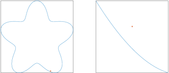
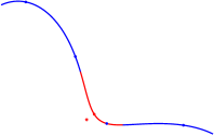
For example, consider a small portion $\mathrm{\Gamma }$ of the starfish

(33) $$\gamma (t)=(1+.25\sin (5t))\exp (\mathrm{i}t),$$

between , and the target point $z=0.45-\mathrm{i}$ (see Fig. 2). For computing the Laplace double layer potential by QBX, as recommended in [4], let $r=l/4$ with $l$ denoting the length of $\mathrm{\Gamma }$. The number of computed coefficients ${\tilde{a}}_m$ at the end of the first phase (num-coeff-phase1) and the number of contributed terms in the approximate potential (11), i.e., $p+1$, for each tolerance $\epsilon$ are listed in Table 1. The differences between the values of these two rows indicate that a considerable portion of computational cost is devoted to computing some coefficients which never come to use.

Figure 2. A portion of the ‘starfish’ geometry (33) between and a target point at $z=0.45-\mathrm{i}$.

$\epsilon$	${10}^{-3}$	${10}^{-4}$	${10}^{-5}$	${10}^{-6}$	${10}^{-7}$	${10}^{-8}$	${10}^{-9}$	${10}^{-10}$	${10}^{-11}$	${10}^{-12}$
num-coeff-phase1	5	6	7	9	10	12	14	15	17	19
$p+1$	3	4	5	5	6	7	8	8	9	10

Table 1. Efficiency of the algorithm proposed in [4] for the Laplace double layer potential at the target point $z=0.45-\mathrm{i}$ and on the ‘starfish’ geometry (33) limited to : The number of computed coefficients ${\tilde{a}}_m$ at the end of Algorithm 1 of [4] (num-coeff-phase1) and the number of contributed terms, $p+1$, for each tolerance $\epsilon$ are computed.

We can revise the above procedure by approximating $a_m$ by ${\tilde{a}}_m$ to the accuracy of $2^{-m-2}\epsilon$ (see Section 2.1) till $|{\tilde{a}}_m{B}_m^r(z,z_0)|$ drops below $\epsilon /4$. Let $m_0>0$ be the smallest integer such that . Then, setting $p:=m_0-1$,

$|e_{\mathrm{T}}|=\left|{\displaystyle \sum _{m=p+1}^{\mathrm{\infty }}}{a}_m{B}_m^r(z,z_0)\right|$ $⪅|a_{m_0}{B}_{m_0}^r(z,z_0)|$

$\le |a_{m_0}-{\tilde{a}}_{m_0}|+|{\tilde{a}}_{m_0}{B}_{m_0}^r(z,z_0)|$

$\le (2^{-m_0}+1)\epsilon /3\le \epsilon /2.$

2.3. Expansion center

Our observations show that position of the target point with respect to the curve $\mathrm{\Gamma }$ affects the efficiency of adaptive QBX. Indeed, the more symmetric the target point is with respect to $\mathrm{\Gamma }$, the earlier the condition is satisfied. Note that this symmetry is not necessary geometrically, and it should be viewed in the sense of parametrization. In order to explain the idea, we need the following lemma.

Lemma 1.

Consider a holomorphic function $h$ on the lines $|\mathrm{\Im }z|=r_0$, for some $r_0>0$. Assume that $h$ satisfies the following conditions in its domain of analyticity: (c1) $\overline{h(z)}=h(\overline{z})$; (c2) either $h(-z)=h(z)$ or $h(-z)=-h(z)$. Then, the real-valued function $\xi$ defined by

(34) $$\xi (t_0)=\left|{\int }_{-1}^{1}h(t-t_0-\mathrm{i}{r}_0)dt\right|,$$

on $[-1,1]$, is even.

Proof.

Change of the variables $t:=-t$ with (c1) and (c2) yields

$\xi (-t_0)$ $=\left|{\displaystyle {\int }_{-1}^1}h(t+t_0-\mathrm{i}{r}_0)dt\right|=\left|{\displaystyle {\int }_{-1}^1}\overline{h(t+t_0-\mathrm{i}{r}_0)}dt\right|$

$=\left|{\displaystyle {\int }_{-1}^1}h(t+t_0+\mathrm{i}{r}_0)dt\right|=\left|{\displaystyle {\int }_{-1}^1}h(-t+t_0+\mathrm{i}{r}_0)dt\right|$

(35) $=\left|{\displaystyle {\int }_{-1}^1}h(t-t_0-\mathrm{i}{r}_0)dt\right|=\xi (t_0).$

∎

Thus, under the assumptions of Lemma 1, $t_0=0$ is a critical point of $\left|{\int }_{-1}^{1}h(t-t_0-\mathrm{i}{r}_0)dt\right|$. In the following, we use Lemma 1 to show that the coefficients $a_m$ in either of the Laplace or the Helmholtz layer potentials, are minimized for almost all $m$, when the projection of the target point on $\mathrm{\Gamma }$, has the preimage in the middle.

2.3.1. Laplace potentials

Assume that $\gamma :[-1,1]\to \mathrm{\Gamma }$ is a parametrization of $\mathrm{\Gamma }$, i.e., $\gamma ([-1,1])=\mathrm{\Gamma }$. Then, for any $m\ge 0$, the coefficient $a_m$, corresponding to the Laplace double layer potential, can be written as

$a_m$ $=-\frac{y^m}{2\pi }{\displaystyle {\int }_{\mathrm{\Gamma }}}{h}_m(w-z_0)n_w\sigma (w)d{s}_w$

(36) $=-\frac{r_0^m}{2\pi \mathrm{i}}{\displaystyle {\int }_{-1}^1}{h}_m\left(\gamma (t)-\gamma (t_0+\mathrm{i}{r}_0)\right){\gamma }^{\prime }(t)\tilde{\sigma }(t)dt,$

where $h_m(z)=z^{-m-1}$, $\tilde{\sigma }=\sigma \circ \gamma$, and $z_0=\gamma (t_0+\mathrm{i}{r}_0)$ is the expansion center. When the length of $\mathrm{\Gamma }$ is small enough and it resembles a straight segment in the complex plain, we can assume that $\tilde{\sigma }$ is almost constant on $[-1,1]$, and $\gamma$ is approximated by a line, i.e.,

(37) $$\gamma (t)\approx bt+q,$$

for some $b,q\in ℂ$. Then,

(38) $$a_m\approx -\frac{r_0^{m}b}{2\pi \mathrm{i}}{h}_m(b)\tilde{\sigma }(0){\int }_{-1}^1{h}_m(t-t_0-\mathrm{i}{r}_0)dt.$$

Similarly, for the Laplace single layer potential

(39) $$a_m\approx -\frac{r_0^m|b|}{2\pi m}{h}_m(b)\tilde{\sigma }(0){\int }_{-1}^1{h}_m(t-t_0-\mathrm{i}{r}_0)dt,m>0.$$

Note that $h_m(z)=z^{-m-1}$ satisfies all the assumptions of Lemma 1. Thus, $t_0=0$, as a critical point of the factor

(40) $${\xi }_m(t_0):=\left|{\int }_{-1}^1{h}_m(t-t_0-\mathrm{i}{r}_0)dt\right|,$$

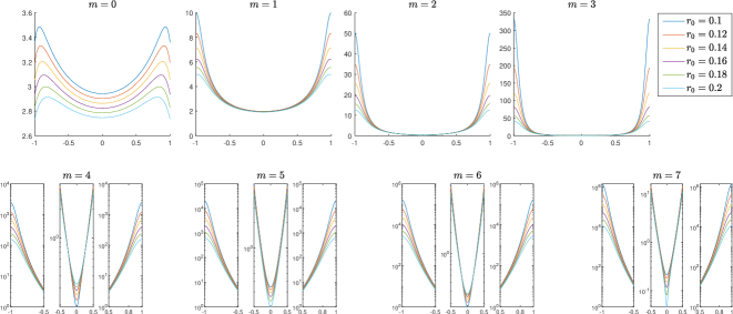
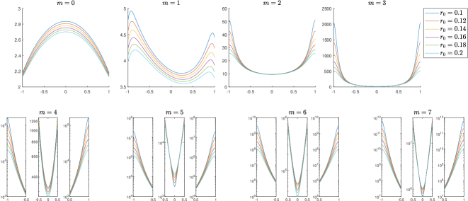
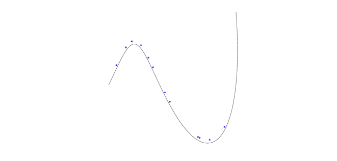
may potentially minimize $|a_m|$, though we could not establish any result about it. However, our numerical experiments are all in accordance with this claim. In Fig. 3, for some different values of $r_0$, we have plotted ${\xi }_m(t_0)$, for $m=0,\mathrm{\dots },7$, as functions of $t_0$.

Figure 3. Graphs of ${\xi }_m(t_0)$, for $m=0,\mathrm{\dots },7$, as functions of $t_0$. As it is seen, the minimum is always occured at $t_0=0$.

Because of the linear assumption (37), one can imply that $\gamma (t_0)$ is almost the closest point of $\mathrm{\Gamma }$ to $z$. Therefore, according to the discussion above, the best position of the near part $\mathrm{\Gamma }$ with respect to the target point $z$ is such that ${\gamma }^{-1}(z_c)$ lies near the midpoint of the preimage ${\gamma }^{-1}(\mathrm{\Gamma })$, where $z_c$ stands for the closest point of $\mathrm{\Gamma }$ to $z$ (see Fig. 4).

Figure 4. Preimage of the panel $\mathrm{\Gamma }$. Here, $z_0=\gamma (t_0+\mathrm{i}{r}_0)$ is the expansion center. It is assumed that the panel $\mathrm{\Gamma }$ is so small that it resembles a stright segment. Thus, becasue of linear assumption (37), one can imply that $\gamma (t_0)\approx z_c$, where $z_c$ is the projection of $z$ (or $z_0$) on $\mathrm{\Gamma }$.

Figure 5. Positions of the target point $z=0.45-\mathrm{i}$ with respect to different near parts $\mathrm{\Gamma }$, corresponding to different partitions of the ‘starfish’ geometry (33) .

Fig	midpoint	$\epsilon$	$p$	Fig	midpoint	$\epsilon$	$p$
		${10}^{-4}$	16			${10}^{-4}$	13
1	5.15	${10}^{-8}$	59	5	5.11	${10}^{-8}$	33
		${10}^{-12}$	93			${10}^{-12}$	94
		${10}^{-4}$	14			${10}^{-4}$	14
2	5.14	${10}^{-8}$	56	6	5.10	${10}^{-8}$	56
		${10}^{-12}$	93			${10}^{-12}$	93
		${10}^{-4}$	13			${10}^{-4}$	15
3	5.13	${10}^{-8}$	32	7	5.095	${10}^{-8}$	58
		${10}^{-12}$	94			${10}^{-12}$	93
		${10}^{-4}$	9			${10}^{-4}$	16
4	5.12	${10}^{-8}$	30	8	5.09	${10}^{-8}$	59
		${10}^{-12}$	92			${10}^{-12}$	93

Table 2. Adaptive QBX for computing the Laplace double layer potential on the panel $\mathrm{\Gamma }$ of the ‘starfish’ geometry (33) with the density function $\sigma \equiv 1$ and the target point $z=0.45-\mathrm{i}$. For each tolerance $\epsilon$, the value of the parameter $p$ at the end of [4, Algorithm 2] depends on the position of $z$ with respect to the near part $\mathrm{\Gamma }$. Here, we consider 6 different situations corresponding to Fig. 5. For each figure (position), the midpoint of the preimage ${\gamma }^{-1}(\mathrm{\Gamma })$ is shown in the column ‘midpoint’. As it is seen, the smallest $p$ always corresponds with Fig. 4, which has the closest midpoint to ${\gamma }^{-1}(z_c)=5.1202$.

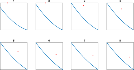
For example, consider the Laplace double layer potential on the ‘starfish’ geometry (33) with the density function $\sigma \equiv 1$ and the target point $z=0.45-\mathrm{i}$. Let $\mathrm{\Gamma }$ be the near part of the boundary, on which adaptive QBX is applied. Depending on the partition of the boundary, position of $z$ with respect to $\mathrm{\Gamma }$ can vary. We consider six different situations (see Fig. 5). Clearly, ${\gamma }^{-1}(z_c)=5.1202$ is fixed in all cases because $z$ is fixed, and it is always in front of the panel $\mathrm{\Gamma }$. In Table 2, we have shown values of the parameter $p$ at the end of [4, Algorithm 2] for some different tolerances $\epsilon$. The midpoint of the preimage ${\gamma }^{-1}(\mathrm{\Gamma })$ is shown in the row ‘midpoint’. It is seen that the smallest $p$ always corresponds with Fig. 4, in which the midpoint 5.12 is closest to ${\gamma }^{-1}(z_c)=5.1202$.

2.3.2. Helmholtz potentials

Figure 6. Graphs of ${\xi }_{1,m}(t_0)$ with $k=0.5$ and $b=1$, for $m=0,\mathrm{\dots },7$, as functions of $t_0$. As it is seen, the minimum is always occured at $t_0=0$ for $m>0$.

Figure 7. Graphs of ${\xi }_{2,m}(t_0)$ with $k=0.5$ and $b=1$, for $m=0,\mathrm{\dots },7$, as functions of $t_0$. As it is seen, the minimum is always occured at $t_0=0$ for $m>0$.

For the Helmholtz single layer potential, the pair

(41) $$({\int }_{-1}^1{h}_{1,m}(t-t_0-\mathrm{i}{r}_0)dt,{\int }_{-1}^1{h}_{2,m}(t-t_0-\mathrm{i}{r}_0)dt)$$

with

(42) $$h_{1,m}(z/b)=H_m^{(1)}\left(k|z|\right)\frac{{|z|}^m}{z^m},h_{2,m}(z/b)=H_{-m}^{(1)}\left(k|z|\right)\frac{z^m}{{|z|}^m}$$

is the $t_0$-dependent factor of the coefficient $a_m$.

Clearly, both $h_{1,m}$ and $h_{2,m}$ satisfy (c2). Note that for any fixed $x\in ℝ$, $J_n(x)\to 0$ as $|n|$ grows. Thus, for the coefficient $a_m$ with larger $m$, the condition (c1) holds approximately, i.e., $\overline{h_{i,m}(z)}\approx h_{i.m}(\overline{z})$, $i=1,2$.

Here again our numerical experiments shows that $t_0=0$ is the minimizer of ${\xi }_{i,m}(t_0)$, for each $i=1,2$, where

(43) $${\xi }_{i,m}(t_0):=\left|{\int }_{-1}^1{h}_{i,m}(t-t_0-\mathrm{i}{r}_0)dt\right|,i=1,2.$$

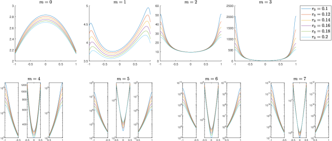
In Fig. 6 and Fig. 7, for fixed $k=0.5$, $b=1$, and some different values of $r_0$, we have plotted ${\xi }_{1,m}(t_0)$ and ${\xi }_{2,m}(t_0)$, respectively, as functions of $t_0$. As it is seen, all the functions are minimized near $t_0=0$ when $m>0$. As expected, the minimizer in each case approaches 0 as the index $m$ grows.

According to the above discussion, we recommend the following strategy for partitioning of the boundary $\partial \mathrm{\Omega }$ with respect to the target point $z$. Find the minimizer $t=t_{\min }$ of $|z-\gamma (t)|$. For a given $dt>0$ small enough, let $I^{\mathrm{near}}=[t_{\min }-dt,t_{\min }+dt]$ be the preimage of the near part, that means that adaptive QBX should be applied on $I^{\mathrm{near}}$, and a traditional quadrature rule should be employed on $[0,2\pi ]\setminus I^{\mathrm{near}}$. It is recommended that $r$ is set to $0.25l$, where $l$ is the length of the near part (see [17]).

3. Algorithms

Assume that an approximation of the density $\sigma (x)$ is available for any $x$ in the panel $\mathrm{\Gamma }\subset \partial \mathrm{\Omega }$. According to the comments in Section Section 2, one can consider the following algorithm as a revision to [4, Algorithms 1,2]:

MAQBX. Modified adaptive QBX based on the Gauss-Legendre quadrature rules, when the panel $\mathrm{\Gamma }$ resembles a straight segment, the target point $z$ lies in the bad annular neighborhood, and $r,n$ are known.
$m=0$, $\kappa =1$
while $E_{\mathrm{C}}(\kappa n,m)>\epsilon /4$ do
$\kappa =\kappa +1$
end while
Apply the ($\kappa n$)-point Gauss-Legendre rule to find ${\tilde{a}}_m$.
${\delta }_m={\tilde{a}}_m\cdot B_m^r(z,z_0)$
$u=0$
repeat
$u=u+{\delta }_m$
$m=m+1$
$\kappa =1$
while $E_{\mathrm{C}}(\kappa n,m)>\max \{2^{-m-2}\epsilon ,{\epsilon }_{\mathrm{mach}}\}$ do
$\kappa =\kappa +1$
end while
Apply the ($\kappa n$)-point Gauss-Legendre rule to find ${\tilde{a}}_m$.
${\delta }_m={\tilde{a}}_m\cdot B_m^r(z,z_0)$
until
return $u_p\left(z\right)=u$ and $p=m-1$

Thus, the main algorithm for computing the layer potential (9) on the whole boundary $\partial \mathrm{\Omega }$ can be described by the following steps:

1. Find the minimizer $t=t_{\min }$ of $|z-\gamma (t)|$.

2. If $|z-\gamma (t_{\min })|$ is small enough, use the following steps; otherwise use a classical quadrature rule for computing the layer potential, and stop.

3. For a given $dt>0$ small enough, set $I^{\mathrm{near}}:=[t_{\min }-dt,t_{\min }+dt]$.

4. Set the half-width $r$ of the bad annular neighborhood of the boundary to $r:=l/4$, where $l$ is the length of $\gamma (t)$, for $t\in I^{\mathrm{near}}$.

5. Apply MAQBX to the near part ${\mathrm{\Gamma }}^{\mathrm{near}}:=\gamma (I^{\mathrm{near}})$, and

6. apply the Gauss-Legendre quadrature to the far part.

Remark 2.

In some cases, we can save some computational efforts in MAQBX. If the target point lies on the boundary, and the potential satisfies a jump condition, it is recommended that QBX should be applied with two expansion centers, say $z_0$ and $z_0^{\prime }$, on the opposite sides of the boundary and the average of the two sided values is considered (see [17, §3.2]). Also for the Helmholtz potentials, one needs to evaluated both $B_m^r$ and $B_{-m}^r$ for each positive $m$. On the other hand, the following equalities hold due to $J_{-n}(x)={(-1)}^n{J}_n(x)$ and ${(|z|/z)}^{-m}=\mathrm{conj}{(|z|/z)}^m$:

$B(-m,z_0)$ $={(-1)}^m\overline{B(m,z_0)},$

$B(m,z_0^{\prime })$ $={(-1)}^{m}B(m,z_0).$

Hence, if we compute $B(m,z_0)$ for some $m$, we can immediately obtain $B(-m,z_0)$, $B(\pm m,z_0^{\prime })$ with no effort.

In BIM, the density function $\sigma$ is unknown, but it can be approximated at any set of discrete points on the boundary $\partial \mathrm{\Omega }$. Divide the boundary into $M$ panels ${\mathrm{\Gamma }}_1,\mathrm{\dots },{\mathrm{\Gamma }}_M$ of an equal length $l$. Let ${\gamma }_m:[-1,1]\to {\mathrm{\Gamma }}_m$ be a parametrization of ${\mathrm{\Gamma }}_m$ for $m=1,\mathrm{\dots },M$, and consider the roots $t_1,\mathrm{\dots },t_n$ of the Legendre polynomial of degree $n$ for some integer $n\ge 1$. The set of $Mn$ Gaussian points ${\gamma }_m(t_j)$, $m=1,\mathrm{\dots },M$, $j=1,\mathrm{\dots },n$, on the boundary form the so-called underlying grid. In adaptive QBX (either the one proposed in this paper or in [4]) the density $\sigma$ must be unsampled even to a finer grid. For this purpose, as proposed in [4], we use the Lagrange interpolation at the underlying grid. More precisely, for computing $\sigma (x)$, where $x$ lies on the panel ${\mathrm{\Gamma }}_m$, we use the Lagrange interpolation of $\tilde{\sigma }:=\sigma \circ {\gamma }_m$ at $t_1,\mathrm{\dots },t_n$. Note that in the main algorithm above, a near part $\mathrm{\Gamma }$ may be different from all ${\mathrm{\Gamma }}_m$ (see Fig. 8). However, the computational cost is not affected by whether the near part coincides with a panel of the underlying grid or not because the density should be resolved at finer grids anyway.

Figure 8. A partition of the ‘starfish’ geometry (33) into 20 panels of an equal length $h$ (the blue dots), and the near part (the red segment) corresponding to the target point located at the red asterisk. The distance of the target point to the curve is less than $h/4$. The red dot on the curve, is located at $\gamma (t_{\min })$, and the interval $[t_{\min }-0.2,t_{\min }+0.2]$ is the preimage of the near part. In this example, the near part does not coincide with any panel of the partition.

4. Numerical experiments

In this section, we carry out some numerical experiments by our desktop PC in order to illustrate efficiency of MAQBX.

4.1. Laplace layer potential evaluation

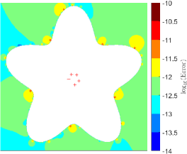
Consider the Laplace double layer potential on the ‘starfish’ geometry (33) with the density function $\sigma \equiv 1$. The exact value of the potential is $-1$ for any target point in the interior domain. As target points, consider a $500\times 500$ grid of a small region near the boundary. In the main algorithm, we choose $dt=0.1$ for each target point, resulting the near part to be always connected. For each target point, we apply MAQBX with $n=16$ to the near part, and the 256-point Gauss-Legendre rule to the far part of the boundary with the tolerances $\epsilon ={10}^{-4},{10}^{-8},{10}^{-12}$ (see Fig. 9 for the absolute error).

Figure 9. Error of MAQBX with $n=16$ and $\epsilon ={10}^{-4},{10}^{-8},{10}^{-12}$ from left to right. The algorithm is applied to the Laplace double layer potential with the density $\sigma \equiv 1$ on the ‘starfish’ geometry (33). The target points are defined by a $500\times 500$ grid of a small region near the boundary. For the far parts, the 256-point Gauss-Legendre rule is employed.

4.2. Comparison to AQBX

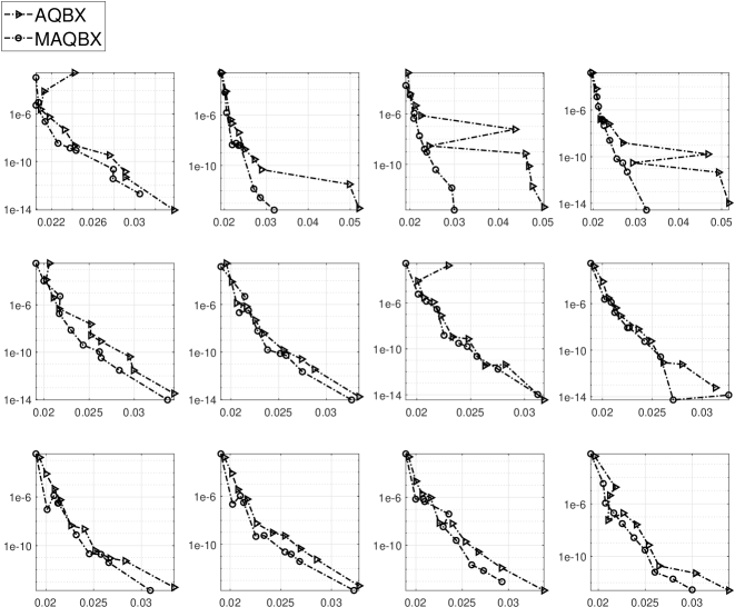
Here, we consider the CPU run-time consumed in implementation of the previous numerical experiment. For twelve target points, selected randomly close to the boundary (see Fig. 11), we implement adaptive QBX of [4] and Algorithms 1 and 2 proposed in this paper. We run each Matlab code 10 times and consider the average of the run-times. In Fig. 10, we compare performance of adaptive QBX with MAQBX. For each algorithm, we plot the relative error as a function of CPU run-time in seconds. As it is seen, MAQBX converges faster than adaptive QBX of [4] in general.

Figure 10. Comparison of adaptive QBX of [4] with MAQBX on the ‘starfish’ geometry (33). Each algorithm is applied to the Laplace double layer potential with the density $\sigma \equiv 1$ at a random target point close to the boundary. Each panel corresponds with a single target point. The positions of the target points are depicted in Fig. 11. The relative error is plotted as a function of the run time in seconds.

Figure 11. The sample target points of Fig. 10.

4.3. Solving a source point scattering problem

Before computing a layer potential, one should approximate the density function $\sigma$ by solving the corresponding boundary integral equation. A more challenging task for adaptive QBX is thus in the context of solving boundary integral equations in which the target points lies on the boundary. In summary, we find a Nyström approximation of $\sigma$ at an underlying grid on the boundary. Then, we use an accurate interpolation to approximate $\sigma$ at a finer grid employed in adaptive QBX for computing the layer potential.

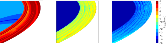
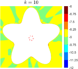
For the wave number $k=0.5$, consider the Helmholtz exterior problem induced by six source points located in the interior of the ‘starfish’ geometry (33). We apply the boundary integral method with the combined field representation

(44) $$u=D_k\sigma +\frac{\mathrm{i}k}{2}{S}_k\sigma ,$$

where $S_k$ and $D_k$ are the Helmholtz single layer and double layer potentials, respectively. As the underlying grid, we divide the boundary into 50 panels of equal length and consider 16 Gauss-Legendre points in each panel. We apply the Nyström method to the corresponding boundary integral equation

(45) $$\left(\frac{1}{2}I+D_k+\frac{\mathrm{i}k}{2}{S}_k\right)\sigma =f,$$

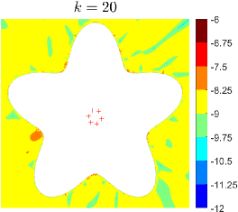
where $f$ is the Dirichlet data induced by the source points. Then, we use the Lagrange interpolation at the underlying grid to obtain an approximation of the density function. In order to solve the Nyström system, we use GMRES with the matrix-vector product carried out by MAQBX with $n=16$ and $\epsilon ={10}^{-12}$. The algorithms with the same parameters are then applied to compute the layer potential as the solution of the source-point problem (see Fig. 12 for the absolute errors). The near part for each target point is bounded in a parameter interval of length $0.02$, and the 512-point Gauss-Legendre rule is applied to the far part.

Figure 12. Error of MAQBX with $\epsilon ={10}^{-12}$, applied to the Helmholtz Dirichlet problem with the wave number $k=0.5$ and Dirichlet data induced to six source points (‘+’) in the interior of the ‘starfish’ geometry (33).

4.4. Higher wavenumbers

Here, we repeat the previous experiment, now for the higher wavenumbers $k=10,20$ and $\epsilon ={10}^{-8}$. The near part for each target point is bounded in a parameter interval of length $0.05$. Other parameters of the algorithm remains the same as in Section 4.3. The results (Fig. 13) show that MAQBX is still practical for scattering problems with higher wavenumbers. The same observation has been reported in [4] for AQBX.

Figure 13. Error of MAQBX with $\epsilon ={10}^{-8}$, applied to the Helmholtz Dirichlet problem with the wave number $k=10,20$ and Dirichlet data induced to six source points (‘+’) in the interior of the ‘starfish’ geometry (33).

5. Conclusions

Adaptive QBX is a robust and accurate tool for computing layer potentials at target points near or on the boundary. In this paper, we have modified the main structure of Algorithms 1,2 of [4] in order to obviate the need to compute extra coefficients $a_m$, which never appear in the truncated expansion of the potential. The modified AQBX is more rapid than AQBX of [4] in practice.