Return to Article Details Multicentric calculus and the Riesz projection

Multicentric calculus and the Riesz projection

Diana Apetrei $^{*}$ Olavi Nevanlinna $^{*}$

November 9, 2015.

$^{*}$ Aalto University, Department of Mathematics and Systems Analysis, P.O.Box 11100, Otakaari 1M, Espoo, FI-00076 Aalto, Finland, email: {Diana.Apetrei,
Olavi.Nevanlinna}@aalto.fi@aalto.fi.

In multicentric holomorphic calculus one represents the function $φ$ using a new polynomial variable $w = p (z)$ in such a way that when it is evaluated at the operator $A,$ then $p (A)$ is small in norm. Usually it is assumed that $p$ has distinct roots. In this paper we discuss two related problems, the separation of a compact set (such as the spectrum) into different components by a polynomial lemniscate, respectively the application of the Calculus to the computation and the estimation of the Riesz spectral projection. It may then become desirable the use of $p (z)^{n}$ as a new variable. We also develop the necessary modifications to incorporate the multiplicities in the roots.

MSC. 30B99, 32E30, 34L16, 47A10, 47A60.

Keywords. multicentric calculus, Riesz projections, spectral projections, sign function of an operator, lemniscates.

A Introduction

Let $p (z)$ be a polynomial of degree $d$ with distinct roots $λ_{1}, \dots, λ_{d}$ . In multicentric holomorphic calculus the polynomial is taken as a new variable $w = p (z)$ and functions $φ (z)$ are represented with the help of a vector-valued function $f$ , mapping $w \mapsto f (w) \in C^{d}$ , [ 9 ] . For example, sets bounded by lemniscates $| p (z) | = ρ$ are then mapped onto discs $| w | \leq ρ$ and for $ρ$ small, $f$ has a rapidly converging Taylor series.

The multicentric representation then yields a functional calculus for operators (or matrices) $A$ , if one has found a polynomial $p$ such that $‖ p (A) ‖$ is small. In fact, denote

V_{p} (A) = {z \in C : | p (z) | \leq ‖ p (A) ‖}

and observe that, by spectral mapping theorem, the spectrum $σ (A)$ satisfies $σ (A) \subset V_{p} (A)$ . If $f$ has a rapidly converging Taylor series for $| w | \leq ‖ p (A) ‖$ , then $φ (A)$ can be written down by a rapidly converging explicit series expansion.

Since $V_{p} (A)$ can have several components, one can define $φ = 1$ in the neighborhood of some components, while $φ = 0$ in a neighborhood of the others. Then $φ (A)$ represents the spectral projection onto the invariant subspace corresponding to the part of the spectrum where $φ = 1$ . The spectral projection satisfies

φ (A) = \frac{1}{2 π i} \int_{γ} (λ I - A)^{- 1} d λ,

where $γ$ surrounds the appropriate components of the spectrum, but the computational approach does not need the evaluation of the contour integral. The coefficients for the Taylor series of $f$ can be computed with explicit recursion from those of $φ$ at the local centers $λ_{j}$ [ 9 ] . The approach also yields a bound for $‖ φ (A) ‖$ by a generalization of the von Neumann theorem for contractions, see [ 7 ] . If the scalar function $φ$ is not holomorphic at the spectrum, the multicentric calculus leads to a new functional calculus to deal with, e.g. nontrivial Jordan blocks [ 10 ] .

In this paper we take a closer look at the computation of spectral projections in finding the stable and unstable invariant subspaces of an operator $A$ . The direct approach would be to ask for a polynomial $p$ with distinct roots such that

V_{p} (A) \cap i R = \emptyset

and then apply the calculus with $φ = 1$ for $Re z > 0,$ respectively $φ = 0$ for $Re z < 0$ . However, we discuss this as two different subjects, one being the separation of the spectrum and the other being the computation of the projection.

In order to discuss the separation, we denote

V (p, ρ) = {z \in C : | p (z) | \leq ρ}

and we let $K = σ (A),$ then we ask what is the minimal degree of a polynomial such that

K \subset V (p, ρ) and V (p, ρ) \cap i R = \emptyset .

A.1

holds. By Hilbert’s lemniscate theorem, see e.g. [ 12 ] , such a polynomial with a minimal degree always exists. We model this question by considering in place of $σ (A)$ two lines parallel to the imaginary axis as follows

K = {z = x + i y : x \in {- 1, 1}, | y | \leq \tan (α)}

and derive a sample of polynomials for which (A.1) holds when $α$ grows. For $α < π / 4,$ the minimal degree is clearly $2$ but in general we are not able to prove exact lower bounds.

Whenever (A.1) holds, then the series expansion of $f$ representing $φ = 1$ for $Re z > 0$ and $φ = 0$ for $Re z < 0$ converges in $p (K),$ and if $σ (A) \subset K$ then we do obtain a convergent expresion for the projection onto to unstable invariant subspace. However, whenever $p (A)$ would be nonnormal, it could happen that $V_{p} (A) \cap i R \neq \emptyset$ , and then we would not get a bound for the projection by the generalization of von Neumann theorem. To overcome this, note that from the spectral radius formula $r (B) = lim ‖ B^{n} ‖^{1 / n}$ in such a case, there does exist an integer $n$ such that with $q = p^{n}$ we have $V_{q} (A) \cap i R = \emptyset$ .

This leads to the other topic discussed in this paper. With $q = p^{n},$ the new variable there are no longer simple zeros and we shall therefore derive the multicentric representations needed in this case. This is done in Section $2$ while the model problem is discussed in Section $3$ . In Section $4$ we present concluding remarks and in the end we discuss a nonnormal small dimensional problem with $q (z) = (z^{2} - 1)^{n}$ .

B Representations and main estimates

B.1 Formulas and estimates

We need the basic formula for expressing a given function $φ (z)$ as a linear combination of functions $f_{j, k} (w^{n})$ when $w = p (z),$ for $n$ a given positive integer.

Let $p (z)$ be the monic polynomial of degree $d$ with distinct roots $λ_{1}, \dots, λ_{d} .$ We denote by $δ_{k} \in P_{d - 1}$ the Lagrange interpolation basis polynomials at $λ_{j}$

δ_{k} (λ) = \frac{1}{p^{'} (λ_{k})} \prod_{j \neq k} (λ - λ_{j}) .

Then the multicentric representation of $φ$ takes the form

φ (z) = \sum_{j = 1}^{d} δ_{j} (z) f_{j} (w), where w = p (z)

B.1

and $f_{j}$ ’s are obtained from $φ$ with the formula [ 7 ]

f_{j} (w) = \sum_{l = 1}^{d} δ_{l} (λ_{j}, w) φ (ζ_{l} (w)),

B.2

where $ζ_{l} (w)$ denote the roots of $p (λ) - w = 0$ and

δ_{l} (λ, w) = \frac{p (λ) - w}{p^{'} (ζ_{l} (w)) (λ - ζ_{l} (w))} .

When $φ$ is holomorphic, $f$ can also be computed from the Taylor coefficients of $φ$ at the local centers $λ_{j}$ . In fact,

f_{j} (w) = \sum_{n = 0}^{\infty} \frac{1}{n!} f_{j}^{(n)} (0) w^{n},

where $f_{j}^{(n)} (0)$ can be computed recursively:

\begin{aligned} (p^{'} (λ_{j}))^{n} f_{j}^{(n)} (0) = \\ = φ^{(n)} (λ_{j}) - \sum_{k = 1}^{d} \sum_{m = 0}^{n - 1} (\binom{n}{m}) δ_{k}^{(n - m)} (λ_{j}) \sum_{l = 0}^{m} b_{m l} (λ_{j}) f_{k}^{(l)} (0) - \sum_{l = 0}^{n - 1} b_{n l} (λ_{j}) f_{j}^{(l)} (0) . \end{aligned}

Here the polynomials $b_{n m}$ are determined by

b_{n + 1, m} = b_{n, m - 1} p^{'} + b_{n m}^{'}

with $b_{n 0} = 0, b_{1, 1} = p^{'}$ and $b_{n m} = 0$ for $m > n$ , see Proposition 4.3 in [ 9 ] .

Remark

Erratum: the last term on the right of (B.3) is missing from the formula (4.2) of [ 9 ] . â–¡

Since the computations for $f_{j}$ ’s are done with power series, we can move to $p (z)^{n} = w^{n},$ because the expansions are done for that variable. Therefore we formulate the next theorem.

Theorem B.1

Suppose $p$ has simple zeros and assume $φ$ is holomorphic in a neighborhood of $V (p, ρ) = {z \in C : | p (z) | \leq ρ}$ and given in the form

φ (z) = \sum_{j = 1}^{d} δ_{j} (z) f_{j} (w), where w = p (z) .

Then

φ (z) = \sum_{j = 1}^{d} δ_{j} (z) [f_{j, 0} (w^{n}) + \dots + w^{n - 1} f_{j, n - 1} (w^{n})],

where $f_{j, k}$ are holomorphic in a neighborhood of the disc $| w | \leq ρ$ and given by

w^{k} f_{j, k} (w^{n}) = \frac{1}{n} {f_{j} (w) + e^{- 2 π i k / n} f_{j} (e^{2 π i / n} w) + \dots + e^{- 2 π i (n - 1) k / n} f_{j} (e^{2 π i (n - 1) / n} w)} .

In order to prove this, we consider a fixed function $f_{j}$ and put $g = f_{j} .$ Then we set

w^{k} g_{k} (w^{n}) = \frac{1}{n} {g (w) + e^{- 2 π i k / n} g (e^{2 π i / n} w) + \dots + e^{- 2 π i (n - 1) k / n} g (e^{2 π i (n - 1) / n} w)}

pointwise.

Proposition B.2

Given an arbitrary $n \in N$ and the functions $g_{i}, i = 0, \dots, n - 1,$ for all $w \in C$ we have:

g (w) = g_{0} (w^{n}) + w g_{1} (w^{n}) + \dots + w^{n - 1} g_{n - 1} (w^{n}) .

Proof â–¼

Using the above formula of $g_{k} (w^{n}),$ for $k = 0, 1, \dots, n - 1,$ we have

\begin{aligned} g_{0} (w^{n}) = & \frac{1}{n} {g (w) + g (e^{2 π i / n} w) + g (e^{4 π i / n} w) + \dots + g (e^{2 π i (n - 1) / n} w)} \\ w g_{1} (w^{n}) = & \frac{1}{n} {g (w) + e^{- 2 π i / n} g (e^{2 π i / n} w) + e^{- 4 π i / n} g (e^{4 π i / n} w) + \dots \\ + e^{- 2 π i (n - 1) / n} g (e^{2 π i (n - 1) / n} w)} \\ w^{2} g_{2} (w^{n}) = & \frac{1}{n} {g (w) + e^{- 4 π i / n} g (e^{2 π i / n} w) + e^{- 8 π i / n} g (e^{4 π i / n} w) + \dots \\ + e^{- 4 π i (n - 1) / n} g (e^{2 π i (n - 1) / n} w)} \\ \dots \\ w^{n - 1} g_{n - 1} (w^{n}) = & \frac{1}{n} {g (w) + e^{- 2 π i (n - 1) / n} g (e^{2 π i / n} w) + e^{- 4 π i (n - 1) / n} g (e^{4 π i / n} w) \\ + \dots + e^{- 2 π i (n - 1)^{2} / n} g (e^{2 π i (n - 1) / n} w)} . \end{aligned}

Summing up all the terms we get

\begin{array}{rcl} \frac{1}{n} n g (w) + \frac{1}{n} g (e^{2 π i / n} w) \sum_{k = 0}^{n - 1} e^{- 2 π i k / n} + \frac{1}{n} g (e^{4 π i / n} w) \sum_{k = 0}^{n - 1} e^{- 4 π i k / n} + \dots \\ + \frac{1}{n} g (e^{2 π i (n - 2) / n} w) \sum_{k = 0}^{n - 1} e^{- 2 π i (n - 2) k / n} + \frac{1}{n} g (e^{2 π i (n - 1) / n} w) \sum_{k = 0}^{n - 1} e^{- 2 π i (n - 1) k / n} \\ = g (w) \end{array}

since all the other terms sum up to zero.

Proof of Theorem B.1 â–¼

It follows now immediately from Proposition B.2 together with the following proposition.

Proposition B.3

If $f_{j}$ is given for $| p (z) | \leq ρ,$ then $f_{j, k},$ $k = 1, \dots, n - 1,$ are defined for $| p (z)^{n} | \leq ρ^{n}$ and

f_{j} (p (z)) = \sum_{k = 0}^{n - 1} p (z)^{k} f_{j, k} (p (z)^{n}), for | p (z) | \leq ρ .

B.-4

Further, if $f_{j} (p (z))$ is analytic for $| p (z) | \leq ρ$ then so are $f_{j, k} (p (z)^{n}) .$

Proof â–¼

First part is proved in Proposition B.2.

For the second part, we assume $f_{j}$ analytic, thus it can be written as a power series

f_{j} (p (z)) = \sum_{m = 0}^{\infty} α_{m} p (z)^{m} .

B.-3

We know that pointwise we have

\begin{array}{rcl} p (z)^{k} f_{j, k} (p (z)^{n}) & = & \frac{1}{n} [f_{j} (p (z)) + e^{- 2 π i k / n} f_{j} (e^{2 π i / n} p (z)) + \dots \\ + e^{- 2 π i (n - 1) k / n} f_{j} (e^{2 π i (n - 1) / n} p (z))] . \end{array}

When we substitute (??) in (B.-2), we get

\begin{aligned} f_{j, 0} (p (z)^{n}) = \\ = \frac{1}{n} [α_{0} + α_{1} p (z) + α_{2} p (z)^{2} + \dots + α_{n} p (z)^{n} + \dots \\ + α_{0} + e^{2 π i / n} α_{1} p (z) + e^{4 π i / n} α_{2} p (z)^{2} + \dots + α_{n} p (z)^{n} + \dots \\ + \dots \\ + α_{0} + e^{2 π i (n - 1) / n} α_{1} p (z) + e^{4 π i (n - 1) / n} α_{2} p (z)^{2} + \dots + α_{n} p (z)^{n} + \dots] . \end{aligned}

Thus $f_{j, 0} (p (z)^{n}) = α_{0} + α_{n} p (z)^{n} + α_{2 n} p (z)^{2 n} + \dots,$ since all the other terms vanish.

We continue with $p (z) f_{j, 1} (p (z)^{n}),$ so we get

\begin{aligned} p (z) f_{j, 1} (p (z)^{n}) = & \frac{1}{n} [α_{0} + α_{1} p (z) + α_{2} p (z)^{2} + \dots + α_{n} p (z)^{n} + \dots \\ + e^{- 2 π i / n} α_{0} + α_{1} p (z) + e^{2 π i / n} α_{2} p (z)^{2} \\ + \dots + e^{2 π i (n - 1) / n} α_{n} p (z)^{n} + α_{n + 1} p (z)^{n + 1} + \dots \\ + \dots \\ + e^{- 2 π i (n - 1) / n} α_{0} + α_{1} p (z) + e^{2 π i (n - 1) / n} α_{2} p (z)^{2} \\ + \dots + e^{2 π i (n - 1)^{2} / n} α_{n} p (z)^{n} + α_{n + 1} p (z)^{n + 1} + \dots] . \end{aligned}

Therefore $f_{j, 1} (p (z)^{n}) = α_{1} p (z) + α_{n + 1} p (z)^{n + 1} + α_{2 n + 1} p (z)^{2 n + 1} + \dots .$

In a similar way it follows that

p (z)^{k} f_{j, k} (p (z)^{n}) = α_{k} p (z)^{k} + α_{n + k} p (z)^{n + k} + α_{2 n + k} p (z)^{2 n + k} + \dots

B.-11

Because all the coefficients $α_{m_{k}},$ for $m_{k} = k, n + k, 2 n + k, 3 n + k, \dots,$ come from $f_{j}$ which is analytic, we know that $lim sup | α_{m_{k}} |^{1 / m_{k}} \leq \frac{1}{ρ},$ therefore we have that $p (z)^{k} f_{j, k} (p (z)^{n})$ is analytic, i.e. a converging power series.

Now, if we factor (??)

p (z)^{k} f_{j, k} (p (z)^{n}) = p (z)^{k} [α_{k} + α_{n + k} p (z)^{n} + α_{2 n + k} p (z)^{2 n} + \dots]

we have that

f_{j, k} (p (z)^{n}) = α_{k} + α_{n + k} p (z)^{n} + α_{2 n + k} p (z)^{2 n} + \dots

is a converging power series, thus is analytic for $| p (z)^{n} | \leq ρ^{n}$ .

Next we need to be able to bound $φ$ in terms of $f_{j, k}$ ’s and vice versa. The first one is straightforward.

Proposition B.4

Denote $L (ρ) = sup_{| p (z) | \leq ρ} \sum_{j = 1}^{d} | δ_{j} (z) | .$ Then

sup_{| p (z) | \leq ρ} | φ (z) | \leq L (ρ) max_{1 \leq j \leq d} \sum_{k = 0}^{n - 1} sup_{| w | \leq ρ} | w^{k} f_{j, k} (w^{n}) | .

The other direction is more involved and we formulate it in the following theorem.

Theorem B.5

Assume $p$ is a monic polynomial of degree $d$ with distinct roots and $s (ρ)$ denotes the distance from the lemniscate $| p (z) | = ρ$ to the nearest critical point of $p,$ $z_{c},$ such that $| p (z_{c}) | > ρ$ . Then there exists a constant $C$ , depending on $p$ but not on $ρ,$ such that if $φ$ is holomorphic inside and in a neighborhood of the lemniscate, then each $f_{j, k}$ is holomorphic for $| w | \leq ρ$ and for $| w | \leq ρ$ , $1 \leq j \leq d$ , $0 \leq k \leq n - 1,$ we have

| w^{k} f_{j, k} (w^{n}) | \leq (1 + \frac{C}{s^{d - 1}}) sup_{| p (z) | \leq ρ} | φ (z) | .

B.-10

For the proof of this statement we need some lemmas. The aim is to bound the representing functions $f_{j, k}$ in terms of the original function $φ$ . To that end we first quote the basic result of bounding $f_{j}$ in terms of $φ$ and then proceed bounding $f_{j, k}$ in terms of $f_{j}$ .

Lemma B.6

(Theorem 1.1 in [ 7 ] ) Suppose $φ$ is holomorphic in a neighborhood of the set ${ζ : | p (ζ) | \leq ρ}$ and let $s$ be as in Theorem B.5. There exists a constant $C$ , depending on $p$ but independent of $ρ$ and $φ$ , such that

sup_{| w | \leq ρ} | f_{j} (w) | \leq (1 + \frac{C}{s^{d - 1}}) sup_{| p (z) | \leq ρ} | φ (z) |, for all j = 1, \dots, d .

Lemma B.7

In the notation above we have

sup_{| w | \leq ρ} | w^{k} g_{k} (w^{n}) | \leq sup_{| w | \leq ρ} | g (w) | .

Proof â–¼

We have

w^{k} g_{k} (w^{n}) = \frac{1}{n} {g (w) + e^{- 2 π i k / n} g (e^{2 π i / n} w) + \dots + e^{- 2 π i (n - 1) k / n} g (e^{2 π i (n - 1) / n} w)} .

The bound follows by taking the absolute values termwise.

Proof of Theorem B.5 â–¼

The proof follows immediately from these two lemmas.

Remark B.8

Gauss-Lucas theorem asserts that given a polynomial $p$ with complex coefficients, all zeros of $p^{'}$ belong to the convex hull of the set of zeros of $p,$ see [ 3 ] . Thus, as soon as $ρ$ is large enough, all the critical points will stay inside the lemniscate whenever the lemniscate is just a single Jordan curve. But when we want to make the separation, we start squeezing the level of the lemniscate and this results in leaving at least one critical point outside. Therefore the $s$ we are measuring is the distance to the boundary from that particular critical point.

If the critical points of $p$ are simple (as they generically are) then the dependency of the distance is inverse proportional and the coefficient in the theorem takes the form

(1 + \frac{C}{s}) .

To see how one can find these constants $C$ and what they describe we will present an example with the computations of $δ_{l} (λ_{j}, w)$ for $p (z) = z^{4} + 1.$ These computations will be used in computing the constants. We also apply them for the Riesz projections.

Example B.9

Let $p (z) = z^{4} + 1$ with roots $λ_{1} = (- 1)^{1 / 4},$ $λ_{2} = (- 1)^{3 / 4},$ $λ_{3} = - (- 1)^{1 / 4}$ and $λ_{4} = - (- 1)^{3 / 4} .$ Let $w = z^{4} + 1.$ Using the formula for $δ_{l} (λ_{j}, w)$ we have:

\begin{array}{rcl} δ_{1} (λ_{1}, w) & = & 1 + \frac{3}{8} w + \frac{19}{64} w^{2} + \frac{33}{128} w^{3} + \dots \\ δ_{1} (λ_{2}, w) & = & - \frac{1 + i}{8} w - \frac{3 + 4 i}{32} w^{2} - \frac{20 + 31 i}{256} w^{3} + \dots \\ δ_{1} (λ_{3}, w) & = & - \frac{1}{8} w - \frac{7}{64} w^{2} - \frac{13}{128} w^{3} + \dots \\ δ_{1} (λ_{4}, w) & = & - \frac{1 - i}{8} w - \frac{3 - 4 i}{32} w^{2} - \frac{20 - 31 i}{256} w^{3} + \dots \\ δ_{2} (λ_{1}, w) & = & - \frac{1}{8} w - \frac{7}{64} w^{2} - \frac{13}{128} w^{3} + \dots \\ δ_{2} (λ_{2}, w) & = & - \frac{1 - i}{8} w - \frac{3 - 4 i}{32} w^{2} - \frac{20 - 31 i}{256} w^{3} + \dots \\ δ_{2} (λ_{3}, w) & = & 1 + \frac{3}{8} w + \frac{19}{64} w^{2} + \frac{33}{128} w^{3} + \dots \\ δ_{2} (λ_{4}, w) & = & - \frac{1 + i}{8} w - \frac{3 + 4 i}{32} w^{2} - \frac{20 + 31 i}{256} w^{3} + \dots \\ δ_{3} (λ_{1}, w) & = & - \frac{1 - i}{8} w - \frac{3 - 4 i}{32} w^{2} - \frac{20 - 31 i}{256} w^{3} + \dots \\ δ_{3} (λ_{2}, w) & = & 1 + \frac{3}{8} w + \frac{19}{64} w^{2} + \frac{33}{128} w^{3} + \dots \\ δ_{3} (λ_{3}, w) & = & - \frac{1 + i}{8} w - \frac{3 + 4 i}{32} w^{2} - \frac{20 + 31 i}{256} w^{3} + \dots \\ δ_{3} (λ_{4}, w) & = & - \frac{1}{8} w - \frac{7}{64} w^{2} - \frac{13}{128} w^{3} + \dots \\ δ_{4} (λ_{1}, w) & = & - \frac{1 + i}{8} w - \frac{3 + 4 i}{32} w^{2} - \frac{20 + 31 i}{256} w^{3} + \dots \\ δ_{4} (λ_{2}, w) & = & - \frac{1}{8} w - \frac{7}{64} w^{2} - \frac{13}{128} w^{3} + \dots \\ δ_{4} (λ_{3}, w) & = & - \frac{1 - i}{8} w - \frac{3 - 4 i}{32} w^{2} - \frac{20 - 31 i}{256} w^{3} + \dots \\ δ_{4} (λ_{4}, w) & = & 1 + \frac{3}{8} w + \frac{19}{64} w^{2} + \frac{33}{128} w^{3} + \dots \end{array}

where $ζ_{l} (w),$ for $l = \overset{―}{1, 4},$ are given by $ζ_{1} (w) = (w - 1)^{1 / 4},$ $ζ_{2} (w) = - (w - 1)^{1 / 4},$ $ζ_{3} (w) = i (w - 1)^{1 / 4}$ and $ζ_{4} (w) = - i (w - 1)^{1 / 4} .$ â–¡

Remark B.10

From Lemma B.6 we see that

| δ_{l}^{(m)} (λ_{k}, w) | \sim \frac{C_{m}}{s^{m + 1}} .

B.-9

where $m$ is the multiplicity of the nearest critical point of $p$ outside the lemniscate. â–¡

To be able to compute the constants $C$ from equation (B.-9) for polynomials of degree $d \geq 4,$ we need to separate the spectrum by perturbing the roots with an angle $ε$ small enough and by dropping the magnitude $ρ$ below $1.$ The perturbations for polynomials of degree $4, 6, 8, 10, 12$ and $14$ are described in the next section.

Note that before the perturbation we have multiple critical points, all inside the lemniscate, except for $0,$ which is on the level curve. After we perturb the roots, one critical point is left outside the lemniscate, while all the others remain inside. Therefore, in our case, the multiplicity $m$ is zero.

From now on we will choose a random value for $ε$ to make some experimental computations. All the computations below will work properly for any other random value $ε$ small enough that ensures the desired separation.

Now, if we choose a random perturbation with, for example, $ε = π / 70,$ we get the following values for the constant $C$

Degree	4	6	8	10	12	14
Constant C	576.4344	1.4665	8.0721	2.2754	12.8520	4.0475

Table B.1 The constant

C

The computations for $\sum | δ_{l} (λ_{k}, w) |$ were made with Mathematica and the values for $s,$ the smallest distance from the lemniscate to the nearest critical point, were computed with the help of Tiina Vesanen that provided a Matlab program. The codes can be found in the appendix of [ 1 ] , which is a preprint version on this article, that contains in appendix material which is not included in this paper. For all these computations one has to choose a value for the level $ρ$ , smaller than $1$ . If one chooses level $ρ = 1,$ then the value for $s$ will be zero, since the lemniscate passes through origin. Therefore we have chosen the minimum value for the level $ρ$ such that the lemniscate separates only in two parts when having a perturbation with $ε = π / 70.$ Hence we have registered the following data

Degree	4	6	8	10	12	14
$\sum \| δ_{l} (λ_{k}, w) \|$	2293.81	6.5122	46.6599	16.3586	83.4547	16.7046
$s$	0.2513	0.2252	0.1730	0.1391	0.1540	0.2423

Table B.2 Experimental values which help in computing the constant

C

in Table B.1.

From the table of constants $C$ one can see that the lemniscate bifurcates differently even with a small $ε .$

Remark B.11

For the quadratic polynomial $p (z) = z^{2} - 1,$ one does not need to perturb the roots, but just to decrease the magnitude of $ρ$ below $1.$ In this case, for example, if the level is $ρ = 0.9$ then one gets $C = 0.2,$ while if the level is $ρ = 0.99$ then $C = 0.6956 .$ â–¡

B.2 Application to Riesz projection

Let $A$ be a bounded operator in a Hilbert space such that

V_{p^{n}} (A) = {z : | p (z)^{n} | \leq ‖ p (A)^{n} ‖} .

In order to compute the Riesz projection we take $φ = 1$ in one of the components and $φ = 0$ in the other components of $V_{p^{n}} (A)$ and

f_{j} (p (z)) = \sum_{k = 0}^{n - 1} p (z)^{k} f_{j, k} (p (z)^{n}) .

B.-8

We shall apply the following theorem, if $φ$ is holomorphic in a neighbourhood of the unit disk $D$ and $A \in B (H),$ then

‖ φ (A) ‖ \leq sup_{D} | φ |,

B.-8

see e.g. [ 11 ] .

From Theorem B.5 we have for $| p (z) | \leq ρ$ that

| p (z)^{k} f_{j, k} (p (z)^{n}) | \leq (1 + \frac{C}{s^{d - 1}}) sup_{| p (z) | \leq ρ} | φ (z) |,

B.-7

and since $f_{j, k}$ are analytic, we can apply (B.-8) to each of them, so with $ρ = ‖ p (A)^{n} ‖^{1 / n}$

‖ f_{j, k} (p (A)^{n}) ‖ \leq sup_{| p (z) | \leq ρ} | f_{j, k} (p (z)^{n}) | .

B.-6

We have,

‖ p (A)^{k} f_{j, k} (p (A)^{n}) ‖ \leq ‖ p (A)^{k} ‖ ‖ f_{j, k} (p (A)^{n}) ‖

and from (B.-6) we get

‖ p (A)^{k} f_{j, k} (p (A)^{n}) ‖ \leq ‖ p (A)^{k} ‖ sup_{| p (z) | \leq ρ} | f_{j, k} (p (z)^{n}) | .

By the Maximum principle we see that

‖ p (A)^{k} ‖ sup_{| p (z) | \leq ρ} | f_{j, k} (p (z)^{n}) | = ‖ p (A)^{k} ‖ ρ^{- k} sup_{| p (z) | \leq ρ} | p (z)^{k} f_{j, k} (p (z)^{n}) | .

Therefore, by (??), we have

‖ p (A)^{k} f_{j, k} (p (A)^{n}) ‖ \leq ‖ (p (A) / ρ)^{k} ‖ (1 + \frac{C}{s^{d - 1}}) sup_{| p (z) | \leq ρ} | φ (z) | .

Substituting now in the decomposition (B.1), $φ (A)$ becomes the Riesz projection and it is bounded by

‖ φ (A) ‖ \leq [(1 + \frac{C}{s^{d - 1}}) \frac{‖ p (A)^{k} ‖}{ρ^{k}} \sum_{j = 1}^{d} ‖ δ_{j} (A) ‖] sup_{| p (z) | \leq ρ} | φ (z) | .

B.-5

Thus we have proven the following theorem.

Theorem B.12

Given a polynomial $p$ of degree $d,$ with distinct roots and a bounded operator $A$ in a Hilbert space, we assume that the "expression"

V_{p^{n}} (A) = {z : | p (z)^{n} | \leq ‖ p (A)^{n} ‖}

has at least two components. Set $ρ = ‖ p (A)^{n} ‖^{1 / n}$ and let $φ$ be a function such that $φ = 1$ in one component of $V_{p^{n}} (A)$ and $φ = 0$ in the others. Let $s$ be the distance from the nearest outside critical point to the boundary of $V_{p^{n}} (A)$ .

Then, considering $f_{j, k}$ as given by Theorem B.1, one has

φ (A) = \sum_{j = 1}^{d} δ_{j} (A) \sum_{k = 0}^{n - 1} p (A)^{k} f_{j, k} (p (A)^{n}),

which is the Riesz spectral projection onto the invariant subspace corresponding to the spectrum inside the component where $φ = 1.$

The bound for the norm of $φ (A)$ is given by (B.-5).

Remark B.13

In applications we will consider $φ = 1$ in the components of $V_{p^{n}} (A)$ that are on the right complex half-plane and $φ = - 1$ in the components on the left complex half-plane. This way the computations are more symmetrical. In this situation there is only one critical point at the origin, which is simple, so we will have $(1 + \frac{C}{s})$ in the formula for the bound of the Riesz projection. â–¡

C Separating polynomials

C.1 Separation tasks

In this section we shall discuss separating issues by lemniscates. To that end, given a polynomial $p$ denote by $V (p, ρ)$ the set

V (p, ρ) = {z \in C : | p (z) | \leq ρ} .

A key result in this context is the following. Let $K \subset C$ be compact and such that $C ∖ K$ is connected. For $δ > 0$ denote further

K (δ) = {z : dist (z, K) < δ} .

Then there exists a polynomial $p$ and $ρ > 0$ such that

K \subset V (p, ρ) \subset K (δ) .

In particular, if $K = K_{1} \cup K_{2}$ and $K_{1} \cap K_{2} = \emptyset$ since $K$ is compact, then for small enough $δ$

K_{1} (δ) \cap K_{2} (δ) = \emptyset

as well. Thus, $V (p, ρ)$ separates the components $K_{1}$ and $K_{2}$ respectively. Suppose that we have two analytic functions $φ_{j}$ , each analytic in $K_{j} (δ)$ . We can view them as just one analytic function

φ : K (δ) \to C,

where $φ$ agrees to $φ_{j}$ on $K_{j} (δ)$ . We are interested in particular in the case where $φ_{j}$ is constant. Multicentric representation then gives a power series which is simultaneously valid in both components.

So, we can ask, for such a separation task what is the smallest degree of a polynomial achieving this.

We model this as follows: Let

K_{1} (δ) = {z = 1 + i y : | y | \leq \tan (δ)}

and $K_{2} (δ)$ symmetrically on the other side of the imaginary axis:

K_{2} (δ) = {z = - 1 + i y : | y | \leq \tan (δ)}

Our first problem concerns the minimal degree of a polynomial $p$ such that

K_{j} (δ) \subset V (p, ρ)

and

V (p, ρ) \cap i R = \emptyset .

This is discussed in the next subsection.

Another natural task is related to existence of a logarithm. So, $C$ is again compact and we assume $0 \notin C$ . Now there exists a single valued logarithm in $C$ if and only if $0$ is in the unbounded component of the complement of $C$ . That is, the set $C$ does not separate origin from infinity. The natural task here is to find a polynomial $p$ such that

C \subset V (p, ρ)

and

0 \notin V (p, ρ) .

As $V (p, ρ)$ is polynomially convex, this suffices for representing the logarithm in $V (p, ρ)$ .

C.2 Model problem

Let $p (z) = z^{d} - 1$ be a monic polynomial of complex variable $z,$ with $| p (z) | = 1.$ The polynomial $p$ can be written as

p (z) = \prod_{j = 1}^{d} (z - e^{i θ_{j}})

where $e^{i θ_{j}}$ are the roots of $p$ and $θ_{j}$ are the angles of the roots. For $d = 4 m,$ $m \geq 1$ we have

p (z) = \prod_{j = 1}^{m} (z - e^{i θ_{j}}) \prod_{j = 1}^{m} (z - e^{- i θ_{j}}) \prod_{j = 1}^{m} (z + e^{i θ_{j}}) \prod_{j = 1}^{m} (z + e^{- i θ_{j}}) .

We are interested to separate the spectrum of $p,$ as discussed earlier in this paper. In this sense, we first check if there are roots laying on the imaginary axis. If so, a rotation with angle $π / d$ is applied so that no roots touch $i R .$

Next we perturb the roots as follows: the four roots that are closest to the imaginary axis (complex roots) are moved along the unit circle towards the real axis with small angle $ε .$ Then the level $ρ$ is slightly decreased with $η .$ This approach is used for polynomials of degree $d \geq 4.$ The quadratic polynomial case is shortly discussed below and cubic polynomial case is presented as a first example.

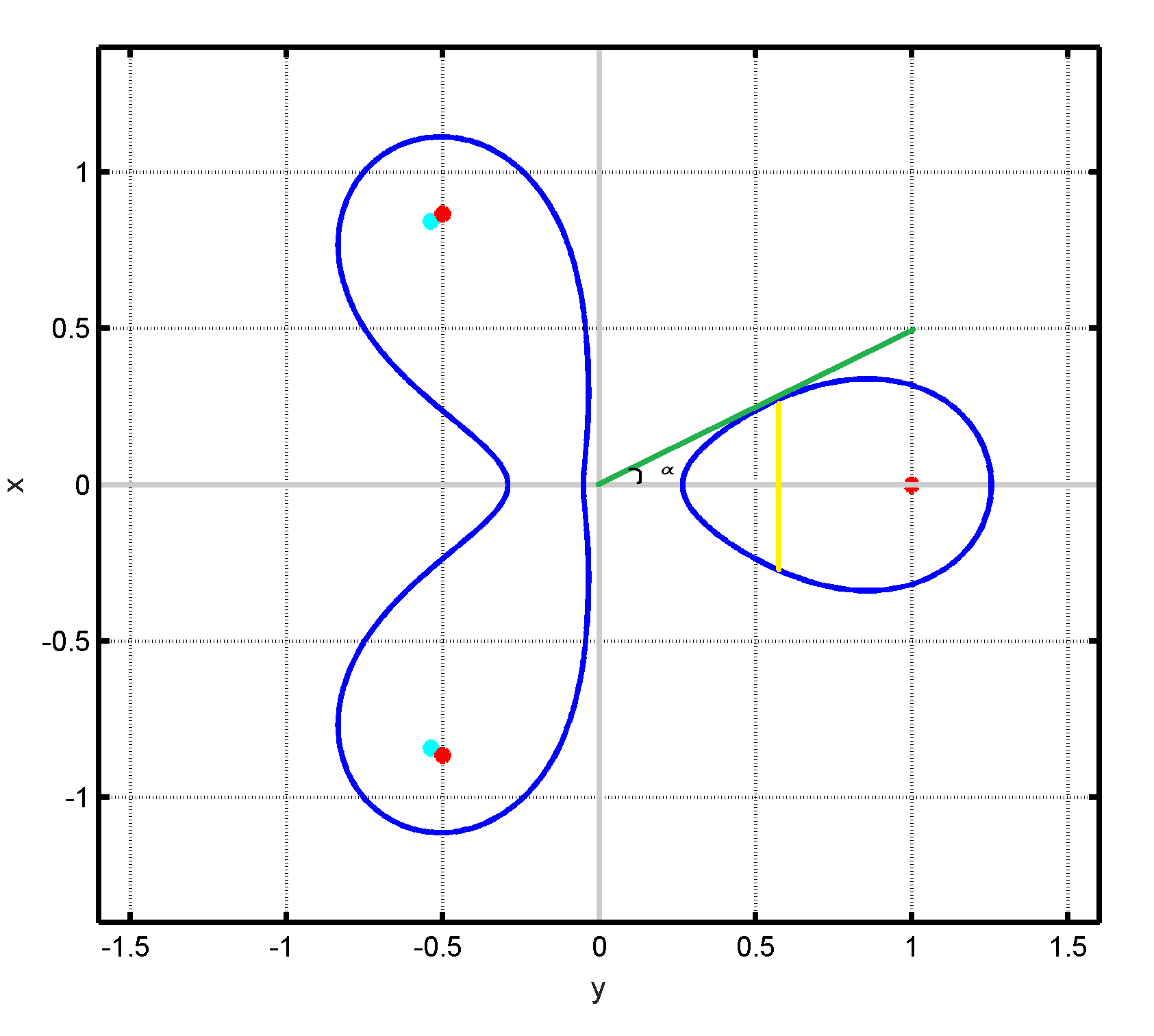
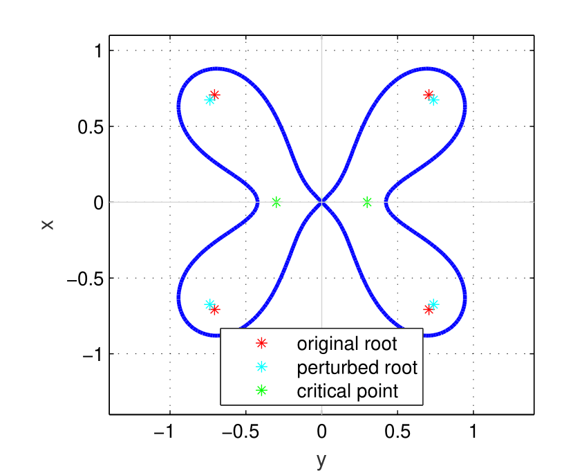
To this end we have to find the maximum $η$ for a chosen $ε$ so that the spectrum gets separated in only two parts, one on the right hand side of the imaginary axis and one on the left hand side. Also we can find the maximum angle $α$ (see Figure 1) such that the spectrum will lay inside our lemniscate.

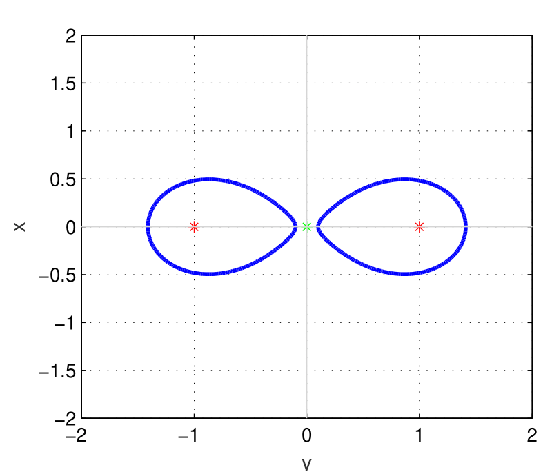
\includegraphics{lemni3level1-004-general.png} — Figure 1 Level 0.996.

Now we analyze some cases. The quadratic polynomial, $p (z) = z^{2} - 1$ is the classical lemniscate and for this one just has to decrease the magnitude $ρ$ to below 1. No perturbation of the roots is needed. For a decrease with $η = 0.01$ of the level we get the picture from Figure 2:

\includegraphics{lemni2level099-new} — Figure 2 Level 0.99.

Example C.1

Let $p (z) = z^{3} - 1$ with roots $e^{2 π i / 3},$ $e^{- 2 π i / 3}$ and $1.$ We apply a perturbation with $ε$ to the complex roots and we get

p_{ε} (z) = (z - e^{i (2 π / 3 + ε)}) (z - e^{- i (2 π / 3 + ε})) (z - 1) .

Thus the lemniscate is $| p_{ε} (z) | = 1 - η .$ For $ε = π / 70$ the resulted picture is shown in Figure ??.â–¡

\includegraphics{lemni3level1-new} — Figure 3 Level 1.

\includegraphics{lemni3level1-004-new} — Figure 4 Level 0.996.

Example C.2

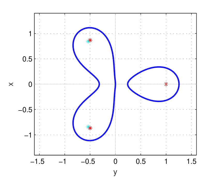
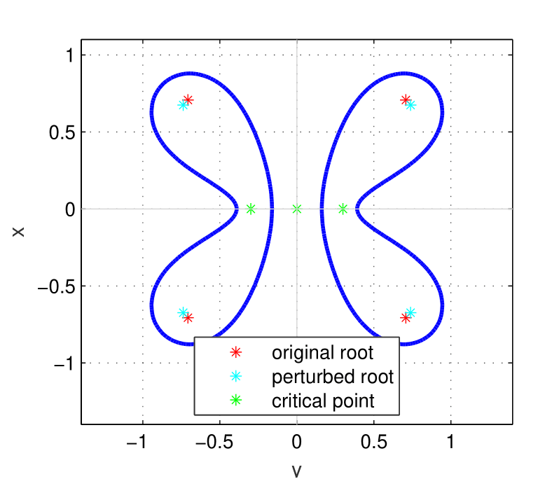
Let $p (z) = z^{4} - 1.$ Since there are roots on the imaginary axis, we have to apply a rotation with $π / 4.$ Thus our polynomial becomes $p (z) = z^{4} + 1.$

Then

p (z) = (z - e^{i θ}) (z - e^{- i θ}) (z + e^{i θ}) (z + e^{- i θ})

where $θ = π / 4,$ so we have

p (z) = (z^{2} - e^{2 i θ}) (z^{2} - e^{- 2 i θ}) = z^{4} - 2 \cos (2 θ) z^{2} + 1.

C.1

Next, we decrease the angle $θ$ with $ε$ small enough and denote the new angle $θ_{ε} = θ - ε .$ For the polynomial with perturbed $θ$ we compute the lemniscate.

We have that

\begin{array}{rcl} e^{2 i θ_{ε}} & = & e^{2 i θ - 2 i ε} = e^{i π / 2 - 2 i ε} \\ = & i (1 - 2 i ε - 2 ε^{2} + \dots) = 2 ε + i (1 - 2 ε^{2} + \dots) . \end{array}

For $z = t \in R$

\begin{array}{rcl} | p_{θ_{ε}} (t) | & = & | t^{2} - 2 ε + i (- 1 + 2 ε^{2} + \dots) |^{2} \\ = & t^{4} - 4 t^{2} ε + 1 + o (ε^{2}) . \end{array}

For $z = i t \in C$

\begin{array}{rcl} | p_{θ_{ε}} (i t) | & = & | (i t)^{2} - 2 ε + i (- 1 + 2 ε^{2} + \dots) |^{2} \\ = & t^{4} - 4 t^{2} ε + 1 + o (ε^{2}) . \end{array}

We write $t = z = x + i y$ in (C.2) and compute the lemniscate $l : | p_{ε} (z) | = 1 - η,$ where $p_{ε} (z) = z^{4} - 2 \cos (2 θ_{ε}) z^{2} + 1$ from (C.1). Thus

\begin{aligned} l : & (x^{2} + y^{2})^{4} + 2 (x^{2} + y^{2})^{2} - 16 x^{2} y^{2} + 16 ε^{2} (x^{2} + y^{2})^{2} \\ - 8 ε (x^{6} + x^{4} y^{2} - x^{2} y^{4} - y^{6} + x^{2} - y^{2}) = 0. \end{aligned}

For $ε = π / 70$ the results are shown in Figure ??. â–¡

\includegraphics{lemni4level1-new} — Figure 5 Level 1.

\includegraphics{lemni4level1-003-new} — Figure 6 Level 0.997.

Similar computations were made for polynomials of degree $6, 8, 10, 12$ and $14,$ and these can be seen in [ 1 ] .

Remark C.3

The goal was to find the maximum angle $α$ such that the spectrum lays inside the lemniscate. For this, one can compute the ratio $a / b,$ where $a$ and $b$ are the length of the lines $a$ and $b$ from Figure 7 below, and hence the angle $α$ is

α = \arctan (a / b) .

C.2

\includegraphics{Ratio_picture.png} — Figure 7 Ratio and angle $α$ .

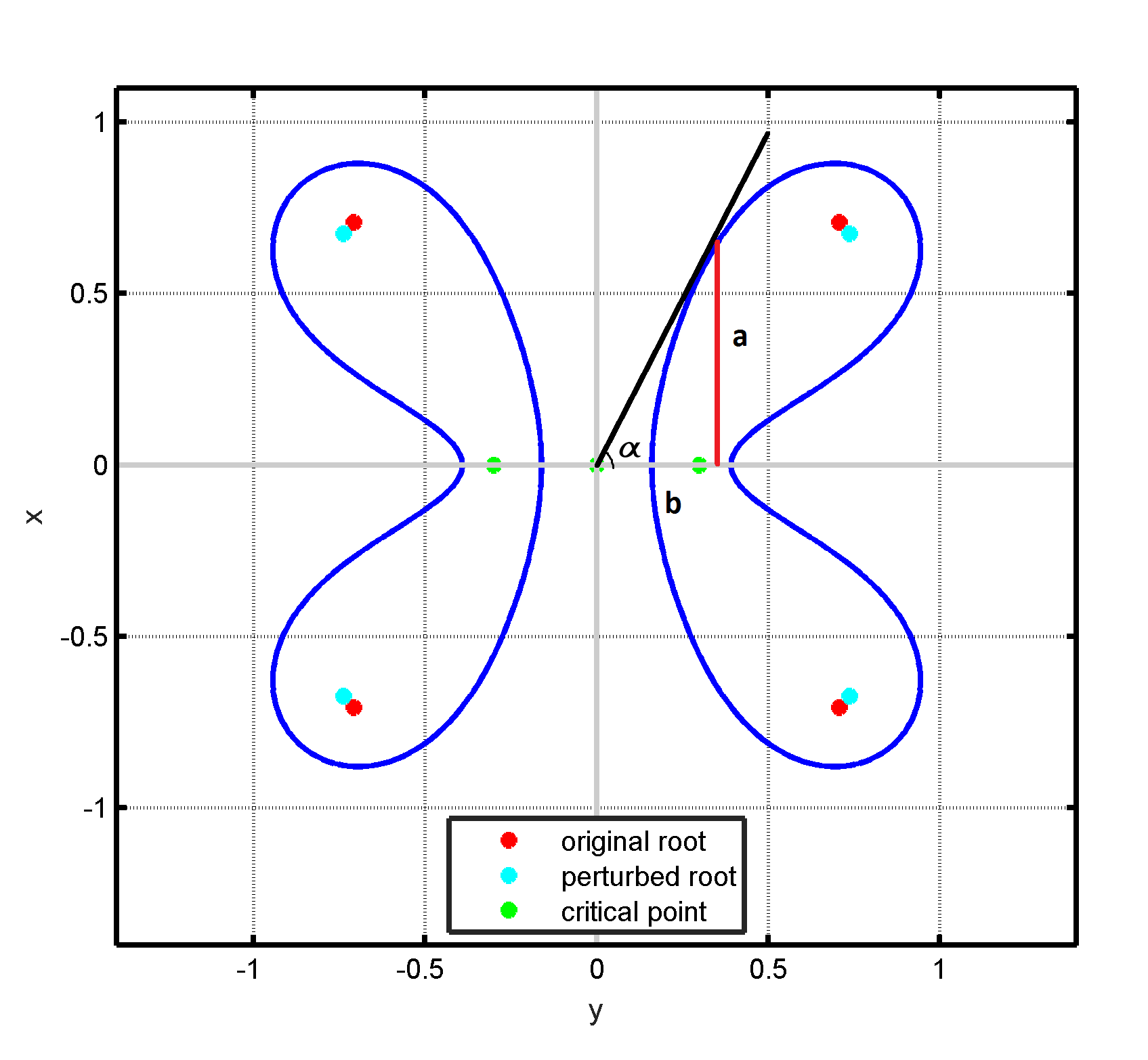
Note that, for a minimum level one might have that the line $a$ cuts the lemniscate, situation that happens even for a slightly perturbation of the level in all the cases with polynomials of degree $d \geq 6.$ Therefore, one has to consider a smaller angle.

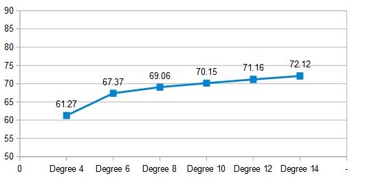
For a minimum level $ρ$ of the lemniscate and a perturbation with $ε = π / 70$ we have the values for the ratio from Table C.1 or from the chart in Fig. 8.

	Degree 4	Degree 6	Degree 8	Degree 10	Degree 12	Degree 14
a	0.5637	0.9040	0.9905	1.0043	0.9973	0.9846
b	0.3090	0.3767	0.3790	0.3624	0.3402	0.3176
a/b	1.8242	2.3997	2.6134	2.7712	2.9315	3.1001

Table C.1 Ratio.

\includegraphics{Ratio_chart_MinLength} — Figure 8 Ratio chart.

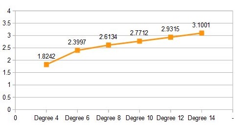
The maximum angle $α$ that we have found is presented in the chart from Figure 9. â–¡

\includegraphics{MaxAngle_MinLength} — Figure 9 Maximum angle $α$ .

Remark C.4

The quadratic polynomial is a special case since the only perturbation applied is decreasing the level. In this case, the maximum angle is when the level $ρ$ is unchanged, in this case $α = 45^{\circ}$ and the minimum angle goes to $0^{\circ}$ when the level is significantly decreased with $η = 0, 99.$ For a slightly change with $η = 0.01$ we have found an angle of ${29.92}^{\circ}$ and for a change with $η = 0.1$ we have registered an angle of ${26.57}^{\circ} .$ â–¡

Remark C.5

For polynomials of degree $d \geq 4$ , it is easy to check the maximum value of $η,$ i.e. the minimum value that the level can have, such that we get the desired separation. For example, if again the perturbation is $ε = π / 70$ we get the values from Table C.2.

Degree	4	6	8	10	12	14
$η$	0.008	0.0078	0.0038	0.0021	0.0022	0.0045

Table C.2 Maximum change

η

of the level

ρ

With these values the lemniscate squeezes next to the closest critical point to the perturbed root. A bigger decrease of the level would force that critical point to get out from the interior of the lemniscate and thus one doesn’t get the desired separation. These estimates may not be the best but they are what we have reached by manipulating the pictures and the resulting pictures can be seen in [ 1 ] . â–¡

D Concluding remarks

In Section $2$ we presented the closed formula and the bound for the Riesz projection, in Section $3$ we described the separation process and in this section one can see how the expansions on the Riesz projection look like when taking $φ = 1$ for the components on the right side of the imaginary axis and $φ = - 1$ for the ones on the left side. We will finish this paper with an example that shows what the effects are on the Riesz projection.

In the appendices of [ 1 ] one can find applications that explicitly compute the series expansions for $f_{j}$ ’s in the decomposition

φ (z) = \sum_{j = 1}^{d} δ_{j} (z) f_{j} (w), w = p (z),

when $φ$ is identically $1$ on the right half plane and $- 1$ on the left half plane, for the quadratic, the quartic, the perturbed quartic polynomial and the polynomial $q (z) = p (z)^{n} = (z^{2} - 1)^{n}$ , respectively.

Remark D.1

In using multicentric calculus a central problem is to find a polynomial $p$ such that $p (A)$ has small norm and, when aiming for Riesz projection, that the lemniscate on the level of $‖ p (A) ‖$ separates the spectrum into different components. This can be done, for example, by minimizing $‖ p (A) ‖$ approximately over a set of polynomials, or, by using a suitable $p$ which has been computed for a neighbouring matrix.

Alternatively, and that is the main topic here, one search for polynomials $p$ such that it is small in a neighbourhood of the spectrum of $A .$ And then computes high enough power $p (A)^{2^{m}}$ such that $‖ p (A)^{2^{m}} ‖^{1 / 2^{m}} \sim ρ (p (A)) .$ â–¡

In the following example we point out with the help of a low-dimensional problem, how the size of coupling can affect on the need of taking a high power of $p (A) .$

Example D.2

Let

A = (\begin{matrix} B & X \\ 0 & - B \end{matrix})

D.1

be a $4 \times 4$ matrix where

B = (\begin{matrix} α & 1 \\ 0 & α \end{matrix})

D.2

and

X = (\begin{matrix} 0 & γ \\ γ & 0 \end{matrix}) .

D.3

In this example we could take $p (z) = z^{2} - α^{2}$ to actually get a closed form for the projection. However, we take $p (z) = z^{2} - 1$ as our polynomial and then the effect of $α > 0$ being close or further away from 1 models the lack of exact knowledge on the spectrum. We are interested in having $‖ p (A)^{n} ‖ < 1$ and ask how the parameters $α$ and $γ$ contribute to the value of $n$ needed. Qualitatively it is clear that such an $n$ exists if and only if $α < \sqrt{2}$ , independently of $γ$ .

Substituting $A$ into $p$ we have

p (A) = (\begin{matrix} C & Y \\ 0 & C \end{matrix}),

where

C = (\begin{matrix} α^{2} - 1 & 2 α \\ 0 & α^{2} - 1 \end{matrix})

and

Y = (\begin{matrix} γ & 0 \\ 0 & - γ \end{matrix}) .

A short computation shows that

p (A)^{n} = (\begin{matrix} C^{n} & n (α^{2} - 1)^{n - 1} Y \\ 0 & C^{n} \end{matrix}) .

Thus, we have

‖ p (A)^{n} ‖ \sim | α^{2} - 1 |^{n - 1} [| α^{2} - 1 | + n (| α | + | γ |)],

so that if $| α^{2} - 1 | ≪ 1$ then a small $n$ shall work. If however, $| α^{2} - 1 | = 1 - ε$ with $0 < ε ≪ 1$ , modelling the case when e.g. spectrum of $A$ is scattered inside the lemniscate, then the behavior is of the nature