Abstract
The goal of this article is to explain some striking discrepancies between the Monte Carlo inferences for flow in heterogeneous aquifers presented in (Shile et al., 2024) and reliable and verifiable results previously published. Comparisons with statistical inferences done within the same numerical setup and using the same benchmark codes demonstrate that quantifiable aspects, such as a too small departure from the linear theory and the decrease of the standard deviations with the increase of the aquifer heterogeneity, cannot be produced with the tools used by the authors.
Authors
Nicolae Suciu
Tiberiu Popoviciu Institute of Numerical Analysis, Romanian Academy, Cluj-Napoca, Romania
Keywords
?
Paper coordinates
N. Suciu, Comment on “Modeling groundwater flow with random hydraulic conductivity using radial basis function partition of unity method” by Shile et al. (2024), Engineering Analysis with Boundary Elements, 169 Part A, (2024), art. no. 105963, https://doi.org/10.1016/j.enganabound.2024.105963
About this paper
Journal
Engineering Analysis with Boundary Elements
Publisher Name
Elsevier
Print ISSN
1873-197X
Online ISSN
0955-7997
google scholar link
Paper (preprint) in HTML form
Comment on “Modeling groundwater flow with random hydraulic conductivity using radial basis function partition of unity method” by Shile et al. (2024)
Abstract
The goal of this article is to explain some striking discrepancies between the Monte Carlo inferences for flow in heterogeneous aquifers presented in (Shile et al., 2024) and reliable and verifiable results previously published. Comparisons with statistical inferences done within the same numerical setup and using the same benchmark codes demonstrate that quantifiable aspects, such as a too small departure from the linear theory and the decrease of the standard deviations with the increase of the aquifer heterogeneity, cannot be produced with the tools used by the authors.
Monte Carlo results of Shile et al. (2024) are compared to previously published ones.
Comparisons are also made with other methods for the same groundwater-flow benchmark.
Striking discrepancy with reliable and verifiable results indicate data fabrication.
1 Introduction
Shile et al., [1] propose a radial basis function (RBF) collocation method to simulate steady-state flows in heterogeneous aquifers. The RBF approach is tested on benchmark problems proposed in [2], using the Matlab codes published in [3]. The hydraulic-head solution is implemented with the codes posted at [4]. Note that these codes are not properly cited, the reference [15] cited by Shile et al., [1], containing a sample Matlab code, does not provide a link to the codes and functions used to solve the RBF interpolation problems presented in their paper. Also, the reference [3] is not cited as a distinct publication, a link to the Git repository being instead added to reference [2], so that the reader cannot know where different elements of the benchmark were taken from.
The benchmark study of Alecsa et al., 2020a [2] is two-fold. First, code verification tests, with manufactured solutions, were conducted for a finite difference method (FDM), a global random walk algorithm (GRW), a finite element method (FEM), and a discontinuous Galerkin method (DGM), as well as for a collocation spectral method (CSM). The realizations of the hydraulic conductivity were provided by a randomization method as analytic space functions. The manufactured solutions were constructed for a fixed realization of the hydraulic conductivity as smooth space functions. These two ingredients favor the CSM, which, using analytical differentiation of the hydraulic conductivity and relatively small numbers of collocations points, yields solutions with an accuracy that is orders of magnitude higher than that of the classical discretization approaches FDM, FEM, GRW, and DGM.
The second part of the study presented in [2] consists of statistical inferences on ensembles of Monte Carlo simulations of transport computed for increasing variance of the log-hydraulic conductivity. This setup, representative for realistic situations, favors the classical discretization methods. Instead, the feasibility of the CSM is limited to small values , due to the need to increase the number of collocation points as the heterogeneity of the hydraulic conductivity increases.
The RBF approach proposed by Shile et al., [1] passes the code verification tests, with errors with respect to the manufactured solutions smaller than those of the classical discretization methods and much larger than the errors of the CSM method presented in [2]. Instead, the statistical inferences results show striking discrepancies with results obtained within the same numerical setup. As shown in the following, the results from [1] cannot be explained by numerical artifacts and there is a strong evidence that the Monte Carlo results are fabricated and the comparisons with previous studies are falsified.
2 Discrepancy with literature results
The numerical procedures used in Monte Carlo simulations of transport in groundwater are validated through comparisons with linear theory and similar numerical approaches (see [5, 6, 7, 8, 2]). One of the mostly used validation test in two-dimensional simulations consists of comparisons of the variances of the longitudinal velocity and of the transverse velocity , defined by
| (1) |
where stands for the average over the ensemble of realizations.
The studies cited above indicate a similar, monotonic increase of the velocity variances with the increase of the variance of the log-hydraulic conductivity above the variances predicted by the linear theory, which, for unit mean longitudinal velocity considered in [2, 1], are given by
| (2) |
The departure from the linear approximation can be illustrated by the semi-analytical second-order approximation, calibrated by Monte Carlo simulations, obtained by Gotovac et al., [8]:
| (3) |
The percentage deviation from the linear approximation (2) will be evaluated in the following by
| (4) |
In Table 1 the results of Shile et al., [1, Table 9] for and exponential correlation of the log-hydraulic conductivity are compared via (4) to the DGM results of Alecsa et al., 2020a [2], to the results from [5, 6, 7], which are close at less than 1.5% to each other [7], and to the second-order approximation (3). The deviation from linear theory of the RBF results sown in Table 1 is one order of magnitude smaller than in earlier published studies.
| RBF | DGM | Refs. [5, 6, 7] | Eqs. (3) | |
|---|---|---|---|---|
| 2.14 | 14.87 | 12.50 | 9.19 | |
| 4.81 | 27.03 | 25.00 | 41.60 |
| Gauss | Exp | |||||||
|---|---|---|---|---|---|---|---|---|
| 0.5 | 1 | 1.5 | 2 | 0.5 | 1 | 1.5 | 2 | |
| 0.00 | 0.80 | 1.2456 | 0.93 | 1.07 | 1.07 | 2.14 | 1.87 | |
| 0.00 | 0.80 | 2.1390 | 3.20 | 0.48 | 3.20 | 4.81 | 4.40 |
| Gauss | Exp | |||||||
|---|---|---|---|---|---|---|---|---|
| 0.5 | 1 | 1.5 | 2 | 0.5 | 1 | 1.5 | 2 | |
| 1.78 | 3.35 | 4.70 | 5.97 | 7.73 | 11.07 | 14.87 | 19.07 | |
| 10.18 | 15.27 | 19.59 | 23.45 | 10.22 | 18.56 | 27.03 | 35.71 |
| 0.5 | 1 | 1.5 | 2 | |
|---|---|---|---|---|
| 3.74 | 6.46 | 9.19 | 11.47 | |
| 15.38 | 29.15 | 42.13 | 53.45 |
| 0.5 | 1 | 1.5 | 2 | |
|---|---|---|---|---|
| -2.58 | -5.06 | -6.46 | -8.61 | |
| -12.91 | -20.09 | -26.25 | -31.96 |
The same striking discrepancy is shown in Table 2 for the results of Shile et al., [1] for the whole range and for both Gaussian and exponential correlations. Tables 3 and 4 show deviations from the linear theory of the DGM results [2] and of the second-order approximation (3), respectively, which are again one order of magnitude larger that those of Shile et al., [1]. And, finally, Table 5 shows that the RBF variances results [1] are systematically smaller than those given by the second-order approximation (3) and the discrepancy increases with .
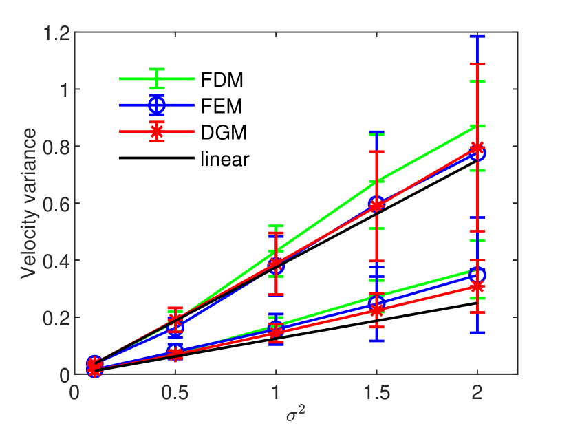
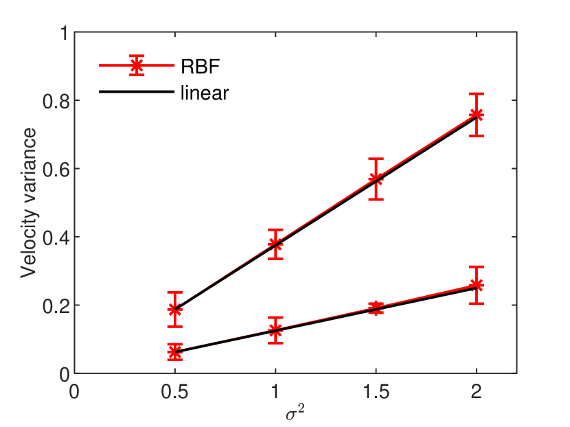
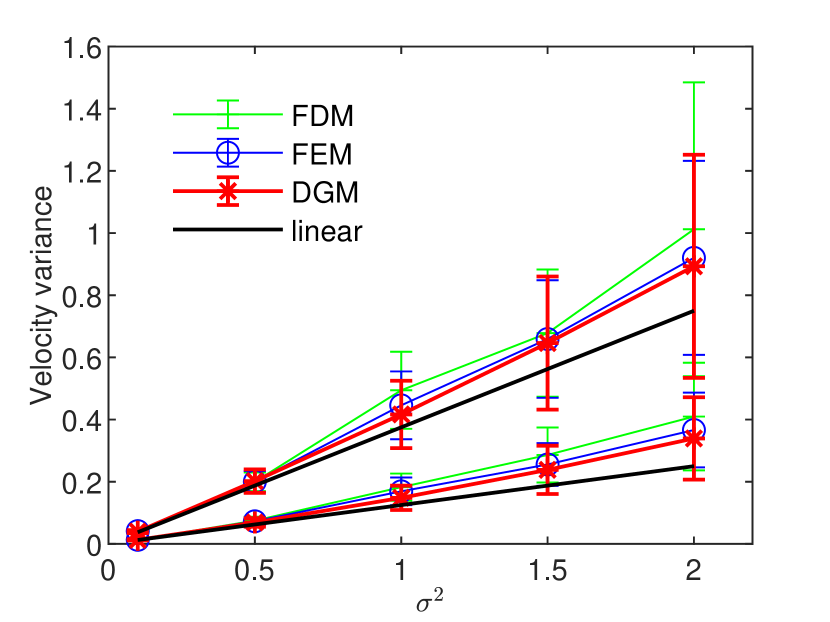
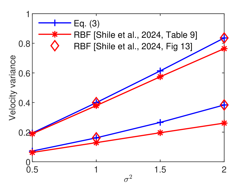
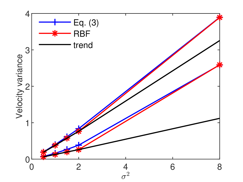
A visual comparison of the results of Shile et al., [1] and earlier results from Alecsa et al., 2020a [2] and Gotovac et al., [8], computed with Eq. (3), is presented in Figs. 2 - 4. Here again one can see that the results presented by Shile et al., [1, Table 9] largely underestimate the departure of the velocity variances from the prediction of the linear theory.
3 Made up results
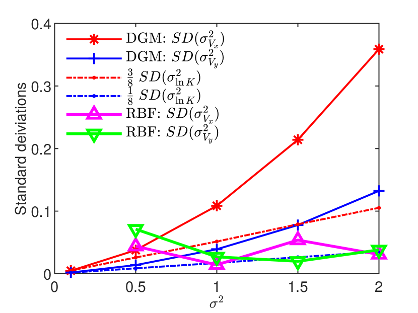
The second striking discrepancy is the non-monotonous behavior of the standard deviations in Shile et al., [1, Table 9], indicated by error bars in Fig. 2 and Fig. 4, as compared with monotonically increasing standard deviations in Fig. 2 and Fig. 4 which present results from [2], that are similar to those published by Bellin et al., [5, Figs. 6a and 6b].
The standard deviations of the ensemble average velocity variances (1) are computed by space averages according to
| (5) |
where stands for the spatial average over the inner core region of the computational domain not affected by the boundary conditions [2]. If the random velocity is statistically homogeneous and do not depend on the spatial variable and their standard deviations defined by (5) vanish. However, since the numerically generated fields are not strictly stationary, the ensemble averages vary from point to point, resulting in a consistent increase of the standard deviations (5) with the increase of , reported in many studies published since the pioneering article of Bellin et al., [5].
Shile et al., [1] used the codes from [3] to generate the random hydraulic conductivity and claim [1, Sect. 4.4] that they used the same numerical setup as Alecsa et al., 2020a [2] and the definition (5) to compute standard deviations of spatially variable velocity variances. Moreover, the code verification tests with two-dimensional manufactured solutions [1, Tables 5 and 6] show that, for , their RBF solver is at least as accurate as the DGM code used in [2, Table 1 and 3]. In these conditions the results obtained with the two approaches should be, in principle, almost identical.
On the other side, the manufactured solutions used in code verification tests are very smooth, with slow oscillations in space (see [1, Fig. 12]), and can be approximated by relatively small numbers of collocation points used in the RBF code, as well as in the CSM code tested in [2]. In these circumstances, the two collocation methods mentioned above benefit from the explicit analytical expression of the hydraulic conductivity used in the benchmark problems [2, Eq. (A3)] to compute its derivatives. Therefore, they outperform the classical approaches which discretize the derivatives (see discussion in [2, Sect. 6]). Instead, the solutions of the homogeneous flow equation used in Monte Carlo simulations are highly heterogeneous and in a first-order approximation follow the shape of the hydraulic conductivity shown in [1, Fig. 2]. Accurate representations of such solutions require more collocation points than in case of the smooth manufactured solutions.
We have thus two possible situations. First, if the same number of collocation points as in code verification tests allows accurate representations of the solutions, as the authors claim in [1, Sect. 4.4], then we are in the case described above, when the RBF and DGM results should be almost identical. This is not the case. The second possibility is that the number of collocation points is not large enough. Then, the representation of the solution is inaccurate and there are realizations with large deviations from the expected almost-laminar behavior (see Supplementary material 2. in [2] which shows “bad” realizations of the CSM collocation method). In this case, larger spatial variability yields larger standard deviations of the velocity variances than the DGM code. This also is not the case (compare Figs. 2 and 2, for Gaussian correlation, and Figs. 4 and 4, for exponential correlation of the field). A first conclusion of this analysis is that the standard deviations presented by Shile et al., [1, Table 9] cannot be produced by their RBF code.
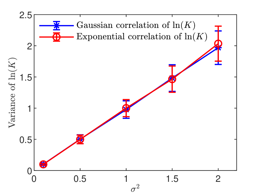
To elucidate the issue of non-monotonous standard deviations shown in Fig. 2 and Fig. 4, I computed ensembles of 100 realizations of the field, for Gaussian and exponential correlations, by using the same parameters and generated with the same codes as in [1, 2], posted in the new folder “Comment on [Shile et al., 2024]” of the Git repository [3]. The estimated mean and standard deviation of variance are plotted in Fig. 6. As expected, the standard deviation increases monotonically with the nominal parameter . With these, the nominal variance used in the Monte Carlo simulations is approximated with a confidence level by
| (6) |
From (6) and (2) we get the following linear approximation of the velocity variances,
| (7) |
If number of random modes used in the field generator and the number of realizations go to infinity, one approaches a statistical homogeneous field, and (7) reduces to (2).
The quantities and in (7) are confidence half-intervals of the mean variances and induced by the statistical inhomogeneity of the field. The same repository also contains ensembles of linear approximations of the corresponding velocity components generated by the Kraichnan method described in [9, Appendix C.3], without the need to solve the flow equation. The comparison presented in Table 6 shows that the confidence intervals from (7) estimate the standard deviations of the velocity variances in a first-order approximation. Since numerical methods to solve the flow equation are prone to errors which increase the statistical inhomogeneity, the estimates from Table 6, computed without solving the flow equation, represent lower bounds of the standard deviations.
| 0.1 | 0.5 | 1 | 1.5 | 2 | |
| 5.17e-03 | 2.59e-02 | 5.14e-02 | 7.90e-02 | 1.05e-01 | |
| 5.07e-03 | 2.69e-02 | 5.35e-02 | 7.82e-02 | 1.06e-01 | |
| 1.72 e-03 | 9.01e-03 | 1.63e-02 | 2.96e-02 | 3.34e-02 | |
| 1.76e-03 | 8.26e-03 | 1.71e-02 | 2.55e-02 | 3.41e-02 |
The detailed comparison of standard deviations for exponential correlation from Fig. 6 shows a total mismatch between the RBF and DGM results. Moreover, the RBF data points show non-monotonous dependence of the standard deviations on and values smaller than the lower bounds and . Since such results cannot be obtained with any numerical method, which was also validated by comparisons with manufactured solutions, the only possible explanation for these flagrant discrepancies of the results from Shile et al., [1, Table 9] is that they are made up.
Summarizing, The results presented by Shile et al., [1] mimic the general feature that the distance between the numerically estimated variance of the velocity components and their linear approximation increases with the increase of , while neglecting three other aspects:
a. the magnitude of the distance from the linear approximation, which is almost the same in previously published studies;
b. the monotonous increase of the standard deviations of the velocity variances;
c. the lower bound of these standard deviations given by the standard deviation of the variance of the field multiplied by 3/8 and 1/8, for longitudinal and transverse velocity, respectively.
4 Falsified comparison with published results
Based on a comparison plotted in their Fig. 13, Shile et al., [1] conclude the presentation of the statistical inferences by stating that “there is good agreement between all the stochastic solutions, supporting the verification of RBFPUM-QR with previously published stochastic results”. However, as we’ll see in the following, this statement is not supported by the numerical results presented by the authors in [1, Table 9].
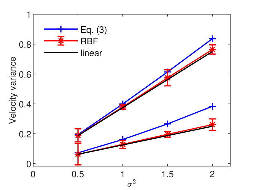
The analysis of the results shown in Figs. 8 and 8 demonstrates that the claim “Fig. 13 confirms that for higher values of , RBFPUM-QR produces results similar to those obtained using the Eqs. (42) and (43)” is false.
First, I compare in Fig. 8 the data points given by Eq. (3) and the RBF data from [1, Table 9] for to the data points from [1, Fig. 13] for and . The distance of 0.123 between the points corresponding to RBF and to Eq. (3) on the lower branch for corresponds to about half the height of the diamond marker in [1, Fig. 13]. As such, this difference should have been visible in [1, Fig. 13] and the marker should have been placed just below the line representing Eq. (43).
The mismatch between the results presented in Shile et al., [1, Table 9 and Fig. 13] is even more obvious in Fig. 8, where the Eq. (3) and the RBF data points from Fig. 8 are completed with the points computed by (3) on which I superposed the RBF points, as in [1, Fig. 13]. The double data points on the upper an lower branches are far away from the trend of RBF points from Fig. 8. This demonstrates that the RBF points cannot be perfectly aligned with the points given by the second-order approximation (3). Hence [1, Fig. 13] falsifies the comparison between the RBF and the previously published results.
5 Conclusions
The article of Shile et al., [1] reproduces, with unnecessary details, the description of the benchmark for flow in saturated aquifers proposed by Alecsa et al., 2020a [2] and the principle of the RBF interpolation approach. The codes from [3] and [4] are further used to conduct code verification tests of the RBF solution. Such tests constitute a necessary preparatory step for applications of the numerical methods to more complex and realistic problems.
The RBF method performs better than classical discretization methods and could be a promising alternative approach in numerical simulations of groundwater flow based on Kraichnan generators of hydraulic conductivity which provide differentiable coefficients of the flow equation. The challenge is to prove that the RBF code can manage realistic spatial heterogeneity conditions which, unlike the smooth manufactured solutions used in code verification tests, require significantly larger numbers of collocation points. Unfortunately, the results of the Monte Carlo simulations presented by Shile et al., [1] are fabricated and the comparison with similar studies, which is supposed to validate the RBF approach, is falsified.
References
- Shile et al., [2024] Shile, F., Ben-Ahmed, E.H, Sadik, M., 2024. Modeling groundwater flow with random hydraulic conductivity using radial basis function partition of unity method. Eng. Anal. Bound. Elem. 163, 237–250. https://doi.org/10.1016/j.enganabound.2024.03.015
- [2] Alecsa, C.D., Boros, I., Frank, F., Knabner, P., Nechita, M., Prechtel, A., Rupp, A., Suciu, N., 2020. Numerical benchmark study for fow in heterogeneous aquifers. Adv. Water Resour., 138, 103558. https://doi.org/10.1016/j.advwatres.2020.103558
- [3] Alecsa, C.D., Boros, I., Frank, Nechita, M., Prechtel, A., Rupp, A., Suciu, N., 2019. FlowBenchmark, Git repository. https://doi.org/10.5281/zenodo.3662401
- Larsson, [2022] Larsson, E., 2022. Radial basis function interpolation - RBF-QR, https://www.it.uu.se/research/scientific_computing/software/rbf_qr
- Bellin et al., [1992] Bellin, A., Salandin, P., Rinaldo, A., 1992. Simulation of dispersion in heterogeneous porous formations: Statistics, first-order theories, convergence of computations. Water Resour. Res. 28(9), 2211–2227. https://doi.org/10.1029/92WR00578
- Salandin and Fiorotto, [1998] Salandin P, Fiorotto V., 1998. Solute transport in highly heterogeneous aquifers. Water Resour. Res. 34(5), 949–961. https://doi.org/10.1029/98WR00219
- de Dreuzy et al., [2007] de Dreuzy, J.-R., Beaudoin, A., Erhel, J., 2007. Asymptotic dispersion in 2D heterogeneous porous media determined by parallel numerical simulations. Water Resour. Res. 43, W10439. https://doi.org/10.1029/2006WR005394
- Gotovac et al., [2009] Gotovac H., Cvetkovic V., Andricevic R., 2009. Flow and travel time statistics in highly heterogeneous porous media. Water Resour. Res. 45, W07402. https://doi.org/10.1029/2008WR007168
- Suciu, [2019] Suciu, N. Diffusion in Random Fields. Applications to Transport in Groundwater, Birkhäuser, Cham, 2019. https://doi.org/10.1007/978-3-030-15081-5
[1] Ben-AhmedE.H. et al. Radial basis function partition of unity method for modelling water flow in porous media, Comput Math Appl, (2018)
[2] ShcherbakovV. et al., Radial basis function partition of unity methods for pricing vanilla basket options, Comput Math Appl., (2016)
[3] KramerP.R. et al., Comparative analysis of multiscale Gaussian random field simulation algorithms, J Comput Phys, (2007)
[4] RoyC.J., Review of code and solution verification procedures for computational simulation, J Comput Phys, (2005)
[5] DriscollT.A. et al., Interpolation in the limit of increasingly flat radial basis functions, Comput Math Appl., (2002)
[6] FornbergB. et al., Some observations regarding interpolants in the limit of flat radial basis functions, Comput Math Appl., (2004)
[7] CainelliO. et al., On the accuracy of classic numerical schemes for modeling flow in saturated heterogeneous formations, Adv Water Resour, (2012)
[8] GotovacH. et al., Adaptive Fup multi-resolution approach to flow and advective transport in highly heterogeneous porous media: Methodology, accuracy and convergence, Adv Water Resour, (2009)
[9] KolyukhinD. et al., Stochastic flow simulation in 3D porous media, Monte Carlo Methods Appl., (2005)
[10] FreezeR.A., A stochastic-conceptual analysis of one-dimensional groundwater flow in nonuniform homogeneous media, Water Resour Res., (1975)
[11] GuoH. et al., Stochastic deep collocation method based on neural architecture search and transfer learning for heterogeneous porous media, Eng Comput, (2022)
[12] AlecsaC.D. et al., Benchmark for numerical solutions of flow in heterogeneous groundwater formations, (2020)
[13] KraichnanR.H., Diffusion by a random velocity field, Phys Fluids, (1970)
[14] KurbanmuradovO.A. et al., Stochastic flow simulation and particle transport in a 2D layer of random porous medium, Transp Porous Media, (2010)
[15] AlecsaC.D. et al., Numerical benchmark study for flow in highly heterogeneous aquifers, Adv Water Resour, (2020)
[16] Safdari-VaighaniA. et al., Radial basis function methods for the rosenau equation and other higher order PDEs, J Sci Comput, (2018)
[17] ShileF. et al., A Meshless Approach for Modeling Water Infiltration in Heterogeneous Soils, (2023)

