Abstract
Solute transport through heterogeneous porous media considered in environmental and industrial problems is often characterized by high Péclet numbers. In this paper we develop a new numerical approach to advection-dominated transport consisting of coupling an accurate mass-conservative mixed finite element method (MFEM), used to solve Darcy flows, with a particle method, stable and free of numerical diffusion, for non-reactive transport simulations. The latter is the efficient global random walk (GRW) algorithm, which performs the simultaneous tracking of arbitrarily large collections of particles on regular lattices at computational costs comparable to those of single-trajectory simulations using traditional particle tracking (PT). MFEM saturated flow solutions are computed for spatially heterogeneous hydraulic conductivities parameterized as samples of random fields. The coupling is achieved by projecting the velocity field from the MFEM basis onto the regular GRW lattice. Preliminary results show that MFEM–GRW is tens of times faster than the full MFEM flow and transport simulation.
Authors
Keywords
Random walk methods; Advection-dominated transport; Porous media
Cite this paper as:
N. Suciu, F.A. Radu, A. Prechtel, F. Brunner, P. Knabner, A coupled finite element-global random walk approach to advection-dominated transport in porous media with random hydraulic conductivity, J. Comput. Appl. Math., 246 (2013), 27-37, doi: 10.1016/j.cam.2012.06.027
References
About this paper
Journal
Journal of Computational and Applied Mathematics
Publisher Name
Elsevier
Online ISSN
0377-0427
Print ISSN
Not available yet.
Google Scholar Profile
[1] U. Jaekel, H. Vereecken, Renormalization group analysis of macrodispersion in a directed random flow, Water Resour. Res. 33 (1997) 2287–2299.
CrossRef (DOI)
[2] H. Schwarze, U. Jaekel, H. Vereecken, Estimation of macrodispersivity by different approximation methods for flow and transport in randomly heterogeneous media, Transp. Porous Media 43 (2001) 265–287.
[3] N. Suciu, C. Vamos, J. Vanderborght, H. Hardelauf, H. Vereecken, Numerical investigations on ergodicity of solute transport in heterogeneous aquifers, Water Resour. Res. 42 (2006) W04409.
CrossRef (DOI)
[4] N. Suciu, C. Vamoş, J. Eberhard, Evaluation of the first-order approximations for transport in heterogeneous media, Water Resour. Res. 42 (2006) W11504.
CrossRef (DOI)
[5] N. Suciu, C. Vamos, F.A. Radu, H. Vereecken, P. Knabner, Persistent memory of diffusion particles, Phys. Rev. E 80 (2009) 061134.
CrossRef (DOI)
[6] N. Suciu, Spatially inhomogeneous transition probabilities as memory effects for diffusion in statistically homogeneous random velocity fields, Phys. Rev. E 81 (2010) 056301.
CrossRef (DOI)
[7] F.A. Radu, N. Suciu, J. Hoffmann, A. Vogel, O. Kolditz, C.-H. Park, S. Attinger, Accuracy of numerical simulations of contaminant transport in heterogeneous aquifers: a comparative study, Adv. Water Resour. 34 (2011) 47–61.
CrossRef (DOI)
[8] P.E. Kloeden, E. Platen, Numerical Solutions of Stochastic Differential Equations, Springer, Berlin, 1999.
[9] C. Vamoş, N. Suciu, H. Vereecken, Generalized random walk algorithm for the numerical modeling of complex diffusion processes, J. Chem. Phys. 186 (2003) 527–544.
CrossRef (DOI)
[10] N. Suciu, C. Vamoş, Global random walk algorithm for diffusion processes, in: A. Skogseid, V. Fasano (Eds.), Random Walks: Principles, Processes and Applications, Nova Science Publishers, New York, 2012, pp. 341–388.
[11] A. Prechtel, P. Knabner, E. Schneid, K.U. Totsche, Simulation of carrier facilitated transport of phenanthrene in a layered soil profile, J. Contam. Hydrol. 56 (2002) 209–225.
CrossRef (DOI)
[12] F.A. Radu, I.S. Pop, P. Knabner, Order of convergence estimates for an Euler implicit, mixed finite element discretization of Richards’ equation, SIAM J. Numer. Anal. 42 (2004) 1452–1478.
CrossRef (DOI)
[13] F.A. Radu, M. Bause, A. Prechtel, S. Attinger, A mixed hybrid finite element discretization scheme for reactive transport in porous media, in: K. Kunisch, G. Of, O. Steinbach (Eds.), Numerical Mathematics and Advanced Applications, Springer-Verlag, 2008, pp. 513–520.
CrossRef (DOI)
[14] F.A. Radu, I.S. Pop, S. Attinger, Analysis of an Euler implicit-mixed finite element scheme for reactive solute transport in porous media, Numer. Methods Partial Differential Equations 26 (2009) 320–344.
CrossRef (DOI)
[15] F. Brunner, F.A. Radu, M. Bause, P. Knabner, Optimal order convergence of a modified BDM1 mixed finite element scheme for reactive transport in porous media, Adv. Water Resour. 35 (2012) 163–171.
CrossRef (DOI)
[16] S.E. Pashenko, K.K. Sabelfeld, D.A. Trubitsyn, Experimental and computer modeling study of stochastic porous filtration of polydispersed aerosols, in: EAC 2008: European Aerosol Conference, Thessaloniki, Greece, 24–29 August, 2008.
[17] F. Delay, P. Ackerer, C. Danquigny, Simulating solute transport in porous or fractured formations using random walk particle tracking: a review, Vadose Zone J. 4 (2006) 360–379.
CrossRef (DOI)
[18] F. Delay, H. Housset-Resche, G. Porei, G. de Marsily, Transport in a 2-D saturated porous medium: a new method for particle tracking, Math. Geol. 28 (1996) 45–71.
CrossRef (DOI)
[19] J. Eberhard, N. Suciu, C. Vamoş, On the self-averaging of dispersion for transport in quasi-periodic random media, J. Phys. A 40 (2007) 597–610.
CrossRef (DOI)
[20] N. Suciu, C. Vamoş, Evaluation of overshooting errors in particle methods for diffusion by biased global random walk, Rev. Anal. Numér. Théor. Approx. 35 (2006) 119–126.
paper on journal website
[21] S. Viswanathan, H. Wang, S.B. Pope, Numerical implementation of mixing and molecular transport in LES/PDF studies of turbulent reacting flows, J. Comput. Phys. 230 (2011) 6916–6957.
CrossRef (DOI)
Paper (preprint) in HTML form
A coupled finite element-global random walk approach to advection-dominated transport in porous media with random hydraulic conductivity
Abstract
Solute transport through heterogeneous porous media considered in environmental and industrial problems is often characterized by high Péclet numbers. In this paper we develop a new numerical approach to advection-dominated transport consisting of coupling an accurate mass-conservative mixed finite element method (MFEM), used to solve Darcy flows, with a particle method, stable and free of numerical diffusion, for non-reactive transport simulations. The latter is the efficient global random walk (GRW) algorithm, which performs the simultaneous tracking of arbitrarily large collections of particles on regular lattices at computational costs comparable to those of single-trajectory simulations using traditional particle tracking (PT). MFEM saturated flow solutions are computed for spatially heterogeneous hydraulic conductivities parameterized as samples of random fields. The coupling is achieved by projecting the velocity field from the MFEM basis onto the regular GRW lattice. Preliminary results show that MFEM-GRW is tens of times faster than the full MFEM flow and transport simulation.
ARTICLE INFO
Article history:
Received 1 February 2012
MSC:
65M12
65M75
76S05
Keywords:
Random walk methods
Advection-dominated transport
Porous media
© 2012 Elsevier B.V. All rights reserved.
1. Introduction
An often used model of transport in highly heterogeneous media, such as groundwater systems, turbulent atmosphere, plasmas, and industrial devices, is based on a stochastic partial differential equation for the concentration field ,
| (1) |
with space variable drift which is a sample of a random velocity field, and a local diffusion coefficient which is assumed constant [1-7]. The normalized concentration solving (1) for the initial condition is the probability density function of the diffusion process described by the Itô stochastic ordinary differential equation
| (2) |
where are deterministic initial positions and are the components of a Wiener process of mean zero and variance 2Dt [8].
In this paper we consider applications to transport in saturated porous media. The time-stationary random velocity field is in this case the solution of the continuity and Darcy equations
| (3) |
where is the hydraulic conductivity of the medium and is the piezometric head [7]. Dirichlet boundary conditions, consisting of constant heads at the inlet and outlet boundaries of the domain, ensure the stationarity in time of the velocity field . The hydraulic conductivity is supplied by various interpretations of field-scale measurements in the form of a spatially distributed random parameter (random field) [1,2].
When solving advection-dominated transport problems associated with (1), like the one considered here, the challenge is to ensure the stability of the solutions and to avoid the numerical diffusion [7]. Therefore, numerical solutions to the Itô equation (2), implemented in PT algorithms, are often used to simulate trajectories of computational particles and to estimate concentrations using particle densities. PT methods are stable, and free of numerical diffusion, and thus suitable for advection-dominated transport problems. However, since the computational costs increase linearly with the number of particles, the estimated concentrations are too inaccurate for large-scale simulations of transport in groundwater. Overcoming the limitations of the sequential PT procedure, the GRW algorithm has no limitations as regards the number of particles [9,3,10]. GRW provides accurate simulations of the concentration field at costs comparable to those of a singletrajectory PT simulation [10].
Some applications of GRW to contaminant transport in groundwater use a first-order approximation in the variance of of the Darcy velocity [3-6]. However, at large variances the approximation fails and exact solutions to the flow problem, such as those obtained by finite element methods [ ], are highly desirable. Here, we propose a coupled approach MFEM-GRW which uses MFEM flow solutions to perform GRW passive transport simulations. The approach will be illustrated by comparisons between MFEM-GRW and the full MFEM solution to both flow and transport, which provide information on the numerical diffusion of the full MFEM scheme for large Péclet numbers. Further, the validated MFEM scheme is used to assess the influence of diffusion coefficients on the filtration efficiency of a simplified model for aerosol filters [16] used to clean the air in ambient and industrial spaces.
The paper is organized as follows. In Section 2 we give a short presentation of the GRW algorithm and some basic implementation details. In Section 3 we introduce the coupled MFEM-GRW approach and present comparisons with the full MFEM scheme and with GRW simulations using linearized flow solutions. Further, we apply the full MFEM scheme to a model air filter in Section 4. Section 5 is devoted to discussions of the results from and perspectives for the coupled approach.
2. The GRW algorithm with reduced fluctuations
A one-dimensional GRW algorithm describing the evolution of particles over the sites of a regular lattice at discrete times indexed by , for particle trajectories governed by a one-dimensional version of the Itô equation (8), distributes the particles according to the rule
| (4) |
where denoting the integer part, are discrete displacements produced by the velocity field and describes the diffusive jumps. The quantities in (4) are Bernoulli random variables associated with the number of particles jumping to the left and to the right from the advected position and is the number of particles that are allowed to stay at the lattice site reached after an advective displacement during the current time step. The distribution of the particles at the next time ( ) is given by
| (5) |
The averages over repeated simulations of the number of particles undergoing diffusive jumps and of the number of particles remaining at the same node after the displacement are given by the relations
| (6) |
where is a rational number. The space step and the time step are related to the diffusion coefficient by the relation
| (7) |
Using (7), for given and , the parameters and can be adjusted to any possible value of the diffusion coefficient .
Particularizing the one-dimensional GRW algorithm (4)-(7) for genuine diffusion ( ), one can easily see that the evolution of the mean number of particles is described by
| (8) |
Since the particles density is proportional to the concentration , the relation (8) has the form of the explicit finite element scheme for the one-dimensional diffusion equation particularizing (1). Since, according to (7)
, the scheme (8) is a consistent approximation of the partial differential diffusion equation and, because (equivalent to von Neumann’s criterion), it is also stable and converges with the order to the exact solution of the initial value problem for the diffusion equation [10].
Considering the case , with and in (7), we get , and (4) describes the number of particles evolving on the lattice according to
| (9) |
which is a weak Euler scheme for the one-dimensional Itô equation (2) with and with Wiener process increments modeled by the noise of constant amplitude and equally probable opposite signs. Hence, describes a superposition of PT simulations in discrete space (on the lattice). This simplified GRW algorithm is by itself a weak Euler scheme in the sense that it does approximate the probability distribution by the particle density but not the trajectories of the Itô process (e.g. [8]). GRW (4)-(7) is further generalized by allowing staying states of the particles ( ) and non-unitary diffusive jumps ( ).
Thought of as a one-dimensional random walk algorithm for genuine diffusion, (9) is a cumulative process consisting of a sum of independent increments , with expectation and variance . By the independence of the increments,
and thus, the computed diffusion coefficient is , i.e., the random walk scheme is unconditionally free of numerical diffusion. The same holds for a general GRW, which is a superposition of weak schemes. To prove that, note that according to (6) is the jump probability and is the local variance of the diffusion process starting at a given lattice site over the time . It follows that the relation (7) is the general definition of diffusion coefficients [8] discretized on the GRW lattice. Whenever numerical diffusion is reported for a random walk scheme [17], it can only be produced by inappropriate implementation options (e.g. [18]).
The GRW algorithm is implemented by creating a procedure for calculating the fluctuating numbers of particles from the right hand side of (4) [9,10]. An efficient implementation, successfully used in large-scale simulations of transport in groundwater [3-6], uses
where is the integer part of and is a random variable taking the values 0 and 1 with probability . Further, the number of particles jumping in the opposite direction, , is determined by (4). In comparison with the exact GRW using Bernoulli random variables, this algorithm reduces the fluctuations of the number of particles to those of a single random walker and, therefore, it has been called "reduced fluctuations" GRW [9]. In the following, by GRW we refer only to this algorithm. From (10) it follows that the computational cost of the GRW simulation for arbitrarily large numbers of particles is roughly speaking the cost for a single PT trajectory multiplied by the number of lattice sites occupied by particles.
We introduce now an efficient implementation of (10) which avoids using random number generators and considerably increases the computational efficiency. It is obtained by redistributing the remainders , appearing in the computation of , and the remainders of the division by 2 of the number of jumping particles to calculate . To ensure the strict conservation of the number of particles, besides the condition requiring that be an integer, related to the use of the parameter , the total number of particles should also be a power of 2 . Nevertheless, we have checked that if the truncation errors are negligible and further increasing over renders the results of the computations presented in the next section indistinguishable in the limit of double precision.
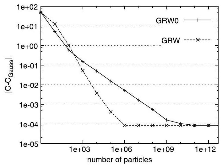
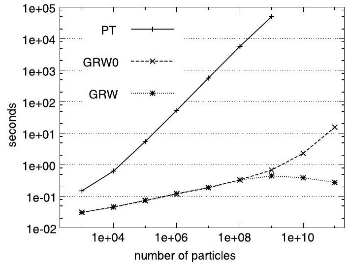
The numerical investigations on convergence presented in Fig. 1 indicate the convergence of the order of the exact GRW solution using Bernoulli repartitions (denoted by GRW0) to the analytical solution of the diffusion equation. For large , when the condition is met, the convergence is of the order as for the finite differences scheme (8). The curves corresponding to the reduced fluctuations algorithm (GRW) in Fig. 1 indicate a faster convergence with , as a consequence of replacing the Bernoulli variables by (10). Fig. 2 shows a comparison of CPU times for the PT code used in , GRW0, and the reduced fluctuation GRW considered in this paper. One can see that the CPU time for PT has a linear increase with . For (ensuring the convergence in Fig. 1) the PT computations already required the use of 256 processors on a parallel machine for about one hour [9].
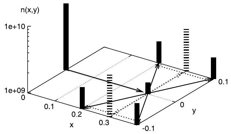
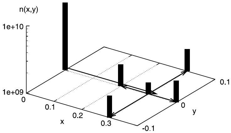
For constant diffusion coefficients the two- and three-dimensional algorithms can be simply built by repeating the onedimensional procedure for all space directions. Fig. 3 illustrates such a two-dimensional GRW algorithm where, after the advective step, the particles execute jumps in the -direction, then jumps in the -direction, both according to the onedimensional rule (4). When the diffusion coefficients vary in space, two different parameters are needed to describe the ratios of particles undergoing jumps [10] and the GRW algorithm follows the rules illustrated in Fig. 4. The following GRW simulations, done for a constant diffusion coefficient (as in Eqs. (1) and (2)), use the two-dimensional algorithm from Fig. 3 in its reduced fluctuations implementation.
3. The coupled MFEM-GRW approach
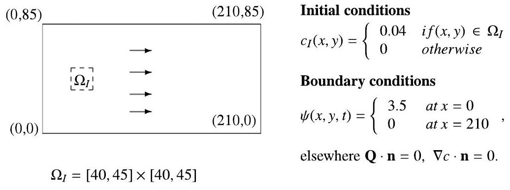
The two-dimensional flow and transport problems associated with (3) and (1) are solved with the MFEM method introduced in [7,15]. The computational domain is and is the final time. The constant diffusion coefficient is set to (lengths are measured in m , times in days, and concentrations are normalized by the maximum initial concentration, as in typical field-scale transport problems for saturated aquifers ). The initial and the boundary conditions for both pressure and concentration are given in Fig. 5.
We consider heterogeneous porous media described using a statistically homogeneous normally distributed loghydraulic conductivity . The fluctuations’ random field , where is the constant expectation of , is homogeneous in a wide sense, with mean zero and a correlation function which only depends on the difference vector , i.e. . The homogeneous random field is generated by
a randomized spectral representation (the Kraichnan method) as a superposition of random sine modes ,
| (11) |
The wavevectors are mutually independent Gaussian random variables, with probability distribution proportional to the spectral density of the field, and the phases are random variables uniformly distributed in the interval . The generated random field has the mean zero, variance , and isotropic correlation described by the function , where ( stands for the Euclidean norm) and is the correlation length.
For the following simulations we fix in (11) the number of modes to , required for accurate transport simulations at the spatial scale considered here [19], and generate a sample of the log-hydraulic conductivity with and . This implies (the geometrical mean which gives the effective conductivity [7]) and a mean longitudinal velocity component . The corresponding global Péclet number is . The computations are carried out on a uniform grid with mean diameter and with a time step . The local Péclet number is . During the whole computation time the solute plume does not reach the boundaries, so the MFEM solution can be compared with GRW simulations for infinite domains.
We also conducted GRW simulations using a first-order approximation of the velocity field. The latter is generated by approximating the linearized solution of the Darcy and continuity equations (3) by a superposition of random periodic modes of the Kraichnan type [1,2]:
| (12) |
The functions in (12) are projectors which ensure the incompressibility of the flow. The similarity with the representation (11) of the log-hydraulic conductivity is a consequence of the proportionality of the corresponding spectral representations [1]. This GRW-Kraichnan approach was successfully used in massive Monte Carlo simulations of transport in aquifers [3-6].
We compute the first and second centered spatial moments of the concentration , defined by
| (13) |
where stands for or and the integrals are computed over the support of . Further, using (13), we compute the half-rates of increase with time of the second moments , which define the effective diffusion coefficients for the transport process [3,5].
The coupled MFEM-GRW approach consists of GRW solutions to transport problems for given velocity fields that are solutions of MFEM schemes. For that, the fluxes over the edges of the Raviart-Thomas elements (triangles) computed at the first MFEM time step are saved in files, together with the coordinates of the corresponding nodes, then read into the GRW code and stored in a vector. Further, one checks to which element each node of the GRW lattice belongs and the velocity components are computed from the three values of the flux over the edges of the element. The coupling algorithm can be summarized as follows:
-
•
compute the MFEM solution to the continuity and Darcy equations (3),
-
•
import the velocity field from the MFEM basis into the GRW lattice:
-
•
find the MFEM element (triangle) to which the lattice point belongs,
-
•
then compute
where are basis coefficients, are position vectors of the corners, and is the area of the triangle,
-
•
use to compute the input parameters and for the GRW rule (4).
The last step of the coupling algorithm requires carefully choosing the space-time discretization to account for velocity variations. We introduce, in addition to the parameters occurring in (7), the parameter defined through
| (14) |
While defines the effective random walk lattice in (4), determines the resolution of the velocity field. When is increased for a better resolution, should also be increased proportionally to , according to (7) and (14). The effective Courant number, defined with respect to the mean velocity , is given by , according to (14). To minimize the overshooting errors [10] the two parameters should be chosen such that the ratio is close to or smaller than 1 . The GRW simulations presented in the following were carried out with particles, which ensure that the results are independent of the number of particles (see Section 2).
To test the coupled MFEM-GRW approach we first consider a single sine mode, i.e. in (11), and a small local Péclet number , obtained by choosing and a mean diameter of the MFEM elements and by modifying the boundary conditions to get a mean longitudinal velocity . With a GRW space step , and , from (14) and (7) one obtains and . The effective Courant number has a desired sub-unity value .
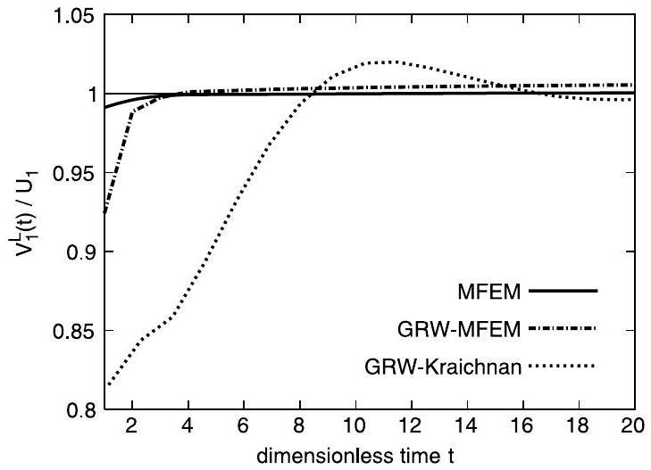
A global indicator of accuracy for both flow and transport solutions in MFEM and for the coupled MFEM-GRW approach is the mean Lagrangian velocity [5,6]
| (15) |
which, as shown in [5] can also be computed by using the time derivative of the center of mass of the solute plume, . The mean Lagrangian velocity was computed using (15) from the MFEM solution and as the time derivative of the center of mass in the GRW simulation.
Figs. 6 and 7 show that the estimations of from the full MFEM and the coupled MFEM-GRW solutions are close to each other, with the exception of the first four dimensionless times , where however the differences, in absolute value, are of the order of day or smaller. Both estimations are close to the mean Eulerian velocity , determined as the spatial average of the MFEM flow solution. By virtue of the ergodicity of the random velocity field and by the self-averaging
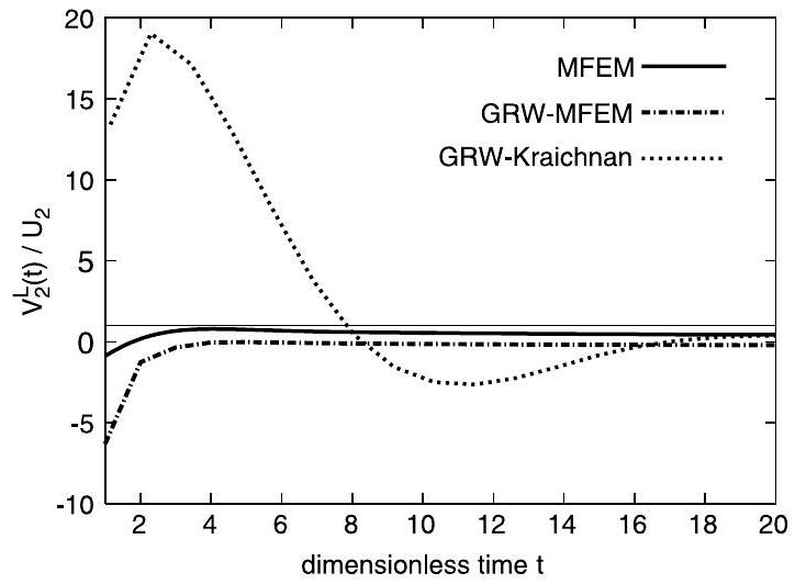
property of the random center of mass, ( ) is also a statistical inference of the ensemble mean Lagrangian velocity [5]. The GRW-Kraichnan estimations show large deviations over more than ten dimensionless times and approach the expected values of only asymptotically.
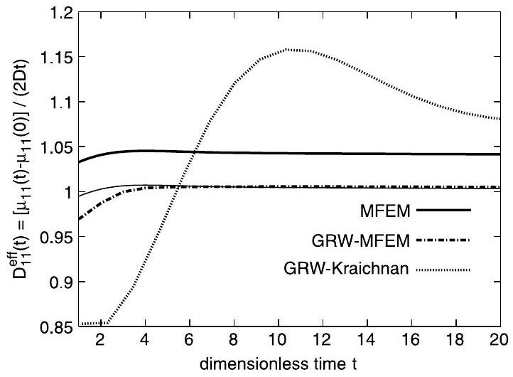
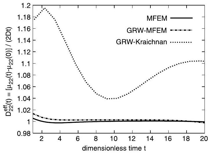
In Figs. 8 and 9 we present the effective coefficients derived from the first two spatial moments (13). The differences between the MFEM and MFEM-GRW estimations are of the order of for longitudinal coefficients and one order of magnitude smaller for the transverse ones. As expected, the GRW-Kraichnan estimations, obtained using the approximation (12) which is valid only for large , show deviations one order of magnitude larger. To investigate the origin of the differences between MFEM and MFEM-GRW estimations, we repeated the computations with a constant velocity given by the estimation ( ) of the mean Eulerian velocity. As shown in Section 2, GRW is free of numerical diffusion and the
estimated diffusion coefficients were identical to in the limit of double precision. We evaluated the numerical diffusion of the MFEM scheme using the relative difference between the coefficient computed from the moments (13) and the nominal diffusion coefficient . We found , almost constant over the simulation duration, for the longitudinal coefficient and a small, negligible mean value for the transverse one. The MFEM estimation of the longitudinal coefficient in the case of variable velocity corrected by subtracting (thin solid line in Fig. 8) becomes almost identical to the MFEM-GRW estimation after a few dimensionless times. Thus, the difference between the two estimations is mainly caused by the numerical diffusion of the MFEM scheme. The small differences at the first time steps of the simulation might be caused by differences of the order of between the MFEM and GRW computations of the initial moments (13). Concluding, the results presented in Figs. 6-9 provide a first validation of the MFEM-GRW approach.
To assess the accuracy of the MFEM method for large-scale simulations in groundwater and to illustrate the utility of the coupled MFEM-GRW approach, we further solved the problem for the numerical setup shown in Fig. 5 , with , and random sine modes in (11). With the chosen parameters , and , we obtained from (7) and (14) the time step , and an effective Courant number close to unity.
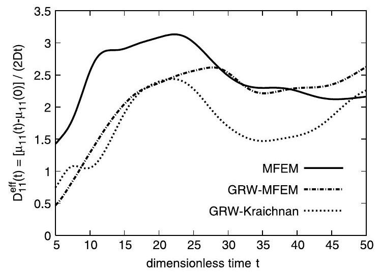
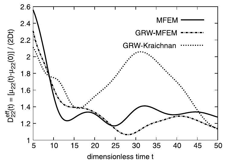
Comparing the full MFEM and the coupled MFEM-GRW solutions from Figs. 10 and 11, we find relative differences of about 1 and 0.2 for longitudinal and transverse effective coefficients, respectively. However, in conditions of rough discretization ( ) and large local Péclet number ( ) these differences are reasonable. Indeed, for , and constant velocity the numerical diffusion of the same MFEM scheme was found to be one order of magnitude larger [7, Table 5]. The smaller differences obtained here suggest the possibility that the highly heterogeneous advection velocity may compensate the intrinsic numerical diffusion of the scheme. This is also supported by the acceptably small confidence intervals of the mean coefficients computed by averaging over an ensemble of 10 realizations of the field generated from (11) [7]. Thus, we conclude that MFEM results presented in Figs. 10 and 11 fulfill usual accuracy requirements for large-scale transport in saturated aquifers [4,20].
The results for the GRW-Kraichnan approach presented in Figs. 10 and 11 show significant deviations from the results of the coupled MFEM-GRW computation. This was already expected because of the approximate nature of the velocity field, which, however, allows good predictions of the asymptotic behavior of the mean effective coefficients [6].
In appreciating the efficiency of the new approach, we note that while the computation of the full MFEM solution presented in Figs. 10 and 11 takes about 10 h , the coupled MFEM-GRW approach, using particles, solves the same problem in about 30 min , from which only 14 s are used for the transport simulation, the most time-consuming part being the projection of the MFEM velocity field onto the GRW lattice. This could be a great advantage in Monte Carlo largescale simulations of passive transport in aquifers, which in the past were generally based on the Kraichnan approximation (12) of the velocity field .
4. MFEM simulations for an air filter model
Since reactions are not yet implemented in GRW, the coupled approach cannot be directly used in reactive transport. Instead, MFEM-GRW can be used to assess the numerical diffusion of the MFEM scheme through comparisons of solutions for passive transport.
Fig. 11 shows that even for the large Péclet number the MFEM solution yields a still acceptable value for the transverse effective diffusion coefficient. The latter controls the dispersive mixing [3] in random porous media which plays an essential role in simulating the behavior of air filter models.
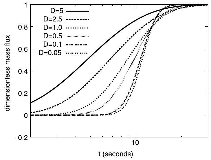
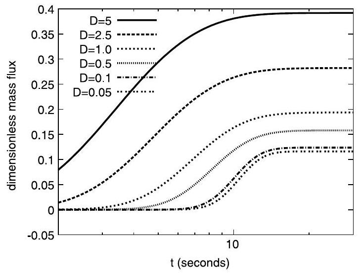
We consider a simplified model for an air filter [16] consisting of a thin two-dimensional domain filled with a porous material, with permittivity modeled as an isotropic, statistically homogeneous random field generated by the randomization algorithm (11). We fixed the mean filtration velocity at , the correlation length of field at 1 cm , and its variance at 0.1 . The diffusion coefficient varies between and , which corresponds, for the fixed MFEM discretization parameter , to a range of local Péclet numbers between 0.1 and 10 . We simulated first the passive transport through the model filter for a continuous incoming flux of air carrying aerosols with a constant, unit intensity. Then, by adding a reaction term on the right side of the transport equation (1), we simulated transport with a uniform retention rate for the same range of diffusion coefficients. The full MFEM computations presented in Figs. 12 and 13 take between 3 and 4 min , so there is no need for a faster MFEM-GRW in this small-scale problem. Instead, we rely on the comparison from Fig. 11 for the correctness of the dispersive mixing.
As shown in Figs. 12 and 13, the diffusion coefficients of the aerosols strongly influence the outgoing flux, and hence the mass of aerosols captured by the filter. Repeating the simulations for various anisotropic fields, as well as for multi-scale fields (i.e. superpositions of fields (11) with increasing correlation lengths), we found that these factors have little importance as compared with the variation of the diffusion coefficients. The latter account for the spectrum of aerosol diameters which is an important parameter involved in designing air filters [16]. The simulations are consistent with measurements done on filters with similar structure and parameters (Anton Latkin, personal communication). Therefore, we expect that MFEM simulations, further developed, e.g. by using the RICHY software [11], to include other microscopic processes expected to have major influence, such as an electrostatic capture, may help in understanding the processes determining the efficiency of filtering.
5. Discussion
The coupled MFEM-GRW approach benefits from the advantages of the MFEM method (high accuracy of the flow solutions, mass conservation, and continuity of the flux over edges [12]) as well as from the high computational speed of the GRW algorithm. For the largest problem investigated in this paper (Figs. 10 and 11) the coupled approach achieved a speed-up of the computations by a factor of 20 . In addition, the new approach completely removes the numerical diffusion inherent to finite element methods.
Although a test of validity has been provided in Section 3, a study of the convergence behavior of the method is still an open issue. A theoretical investigation on the convergence of the GRW algorithm, in terms of von Neumann’s criterion and the Courant number, can be done only for constant velocity, like in the case of the genuine diffusion problem discussed in Section 2. For transport in random media, as in the example presented in Section 3, when GRW is no longer equivalent to a finite difference scheme, a possible suggestion would be to investigate the average behavior of the ensemble of GRW solutions for statistically homogeneous random velocity fields. Numerical convergence investigations are however feasible even in deterministic cases or for single-velocity realizations. They could use as reference solutions, for the same MFEM velocity fields, the solutions of the slower but more accurate biased GRW algorithm [ ] which is equivalent to a finite difference scheme even for variable velocity fields.
The MFEM-GRW approach could be a useful tool in assessing the numerical diffusion for MFEM schemes which are further applied to the simulation of more complex transport processes taking place in the same velocity field, as illustrated by Sections 3 and 4 in this paper. Another envisaged application aims at producing highly accurate and efficient Monte Carlo simulations for large-scale passive transport problems specific to subsurface hydrology [3]. Nonetheless, an MFEM-GRW approach can be proposed as an alternative to the particle-mesh method used to solve the parabolic partial differential equation for the probability density of the random concentration in modeling turbulent transport [21].
Acknowledgment
This work was supported by Bundesministerium für Bildung und Forschung under grant RUS 09/B12.
References
[1] U. Jaekel, H. Vereecken, Renormalization group analysis of macrodispersion in a directed random flow, Water Resour. Res. 33 (1997) 2287-2299.
[2] H. Schwarze, U. Jaekel, H. Vereecken, Estimation of macrodispersivity by different approximation methods for flow and transport in randomly heterogeneous media, Transp. Porous Media 43 (2001) 265-287.
[3] N. Suciu, C. Vamos, J. Vanderborght, H. Hardelauf, H. Vereecken, Numerical investigations on ergodicity of solute transport in heterogeneous aquifers, Water Resour. Res. 42 (2006) W04409.
[4] N. Suciu, C. Vamoş, J. Eberhard, Evaluation of the first-order approximations for transport in heterogeneous media, Water Resour. Res. 42 (2006) W11504.
[5] N. Suciu, C. Vamos, F.A. Radu, H. Vereecken, P. Knabner, Persistent memory of diffusion particles, Phys. Rev. E 80 (2009) 061134.
[6] N. Suciu, Spatially inhomogeneous transition probabilities as memory effects for diffusion in statistically homogeneous random velocity fields, Phys. Rev. E 81 (2010) 056301.
[7] F.A. Radu, N. Suciu, J. Hoffmann, A. Vogel, O. Kolditz, C.-H. Park, S. Attinger, Accuracy of numerical simulations of contaminant transport in heterogeneous aquifers: a comparative study, Adv. Water Resour. 34 (2011) 47-61.
[8] P.E. Kloeden, E. Platen, Numerical Solutions of Stochastic Differential Equations, Springer, Berlin, 1999.
[9] C. Vamoş, N. Suciu, H. Vereecken, Generalized random walk algorithm for the numerical modeling of complex diffusion processes, J. Chem. Phys. 186 (2003) 527-544.
[10] N. Suciu, C. Vamoş, Global random walk algorithm for diffusion processes, in: A. Skogseid, V. Fasano (Eds.), Random Walks: Principles, Processes and Applications, Nova Science Publishers, New York, 2012, pp. 341-388.
[11] A. Prechtel, P. Knabner, E. Schneid, K.U. Totsche, Simulation of carrier facilitated transport of phenanthrene in a layered soil profile, J. Contam. Hydrol. 56 (2002) 209-225.
[12] F.A. Radu, I.S. Pop, P. Knabner, Order of convergence estimates for an Euler implicit, mixed finite element discretization of Richards’ equation, SIAM J. Numer. Anal. 42 (2004) 1452-1478.
[13] F.A. Radu, M. Bause, A. Prechtel, S. Attinger, A mixed hybrid finite element discretization scheme for reactive transport in porous media, in: K. Kunisch, G. Of, O. Steinbach (Eds.), Numerical Mathematics and Advanced Applications, Springer-Verlag, 2008, pp. 513-520.
[14] F.A. Radu, I.S. Pop, S. Attinger, Analysis of an Euler implicit-mixed finite element scheme for reactive solute transport in porous media, Numer. Methods Partial Differential Equations 26 (2009) 320-344.
[15] F. Brunner, F.A. Radu, M. Bause, P. Knabner, Optimal order convergence of a modified BDM1 mixed finite element scheme for reactive transport in porous media, Adv. Water Resour. 35 (2012) 163-171.
[16] S.E. Pashenko, K.K. Sabelfeld, D.A. Trubitsyn, Experimental and computer modeling study of stochastic porous filtration of polydispersed aerosols, in: EAC 2008: European Aerosol Conference, Thessaloniki, Greece, 24-29 August, 2008.
[17] F. Delay, P. Ackerer, C. Danquigny, Simulating solute transport in porous or fractured formations using random walk particle tracking: a review, Vadose Zone J. 4 (2006) 360-379.
[18] F. Delay, H. Housset-Resche, G. Porei, G. de Marsily, Transport in a 2-D saturated porous medium: a new method for particle tracking, Math. Geol. 28 (1996) 45-71.
[19] J. Eberhard, N. Suciu, C. Vamoş, On the self-averaging of dispersion for transport in quasi-periodic random media, J. Phys. A 40 (2007) 597-610.
[20] N. Suciu, C. Vamoş, Evaluation of overshooting errors in particle methods for diffusion by biased global random walk, Rev. Anal. Numér. Théor. Approx. 35 (2006) 119-126.
[21] S. Viswanathan, H. Wang, S.B. Pope, Numerical implementation of mixing and molecular transport in LES/PDF studies of turbulent reacting flows, J. Comput. Phys. 230 (2011) 6916-6957.
- •