Abstract
In this paper a Laguerre collocation type method based on usual Laguerre functions is designed in order to solve high order nonlinear boundary value problems as well as eigenvalue problems, on semi-infinite domain. The method is first applied to Falkner–Skan boundary value problem. The solution along with its first two derivatives are computed inside the boundary layer on a fine grid which cluster towards the fixed boundary. Then the method is used to solve a generalized eigenvalue problem which arise in the study of the stability of the Ekman boundary layer. The method provides reliable numerical approximations, is robust and easy implementable. It introduces the boundary condition at infinity without any truncation of the domain. A particular attention is payed to the treatment of boundary conditions at origin. The dependence of the set of solutions to Falkner–Skan problem on the parameter embedded in the system is reproduced correctly. For Ekman eigenvalue problem, the critical Reynolds number which assure the linear stability is computed and compared with existing results. The leftmost part of the spectrum is validated using QZ as well as some Jacobi–Davidson type methods.
Authors
Călin-Ioan Gheorghiu
(Tiberiu Popoviciu Institute of Numerical Analysis, Romanian Academy)
Keywords
References
See the expanding block below.
Cite this paper as
C.I. Gheorghiu, Laguerre collocation solutions to boundary layer type problems. Numer. Algor., 64 (2013) 385-401
doi: 10.1007/s11075-012-9670-y
About this paper
Print ISSN
1017-1398
Online ISSN
1572-9265
Google Scholar Profile
google scholar link
Paper (preprint) in HTML form
Accurate Laguerre collocation solutions to boundary layer type problems
Abstract
In this paper a Laguerre collocation type method based on generalized Laguerre functions is designed in order to solve high order nonlinear boundary value problems as well as eigenvalue problems, on semi-infinite domain. The method is first applied to Falkner-Skan boundary value problem. The solution along with its first two derivatives are computed inside the boundary layer on a fine grid which cluster towards the fixed boundary. Then the method is used to solve a generalized eigenvalue problem which arise in the study of the stability of the Ekman boundary layer. The method is accurate, robust and easy implementable. It introduces the boundary condition at infinity without any truncation of the domain and treats efficiently and directly the nonlinearities of the equations. A particular attention is also payed to the treatment of boundary conditions at origin. The dependence of the set of solutions to Falkner-Skan problem on the parameter embedded in the system is reproduced correctly. The particular Blasius case is considered as a benchmark problem. For Ekman eigenvalue problem, the critical Reynolds number which assure the linear stability is computed and compared with existing results. The leftmost part of the spectrum is validated using Arnoldi as well as some Jacobi-Davidson type methods. The pseudospectrum of the algebraic generalized eigenvalue problem involved suggests the limitations of the linear stability analysis.
Keywords:
Collocation · Usual Laguerre functions · Semi-infinite domain · Falkner–Skan equation · Ekman eigenvalue problem · Leftmost eigenpair1 Introduction
The difficulties as well as possible remedies in solving boundary value problems and eigenvalue problems on unbounded domains are thoroughly considered in the well known monograph of Boyd JPB and recent monograph of Shen, Tang and Wang STW . There exists a vast literature on domain truncation type methods, the most used methods for such problem, but considerable less rigorous estimations of the domain truncation errors. Domain truncation was coupled with different techniques such as shooting, finite differences as well as Galerkin schemes. Galerkin or collocation methods, based on the Laguerre functions, and the Chebyshev polynomials with various mappings, are the other two alternatives. The application of these methods restricts to various first and second order differential problems (see the above mentioned works and also BRB and Shen1 ).
Thus, the main aim of this paper is to accurately solve higher order boundary layer type problems, including generalized eigenvalue ones, by a collocation method based on generalized Laguerre functions. The method is general, fairly efficient in imposing the boundary conditions in origin and at infinity, easy implementable and require no domain truncation. Actually, the boundary conditions at infinity are exactly satisfied by Laguerre functions and the conditions at zero are introduced by a removing technique of independent boundary conditions due to J. Hoepffner JH . Once the differentiation matrices are accurate computed the method is directly implementable. Throughout this paper the Laguerre differentiation matrices are those provided by the paper of Weideman and Reddy WR (see also the monograph of Funaro F ).
We will analyze two distinct, difficult, and representative boundary layer type problems. The first one is the general Falkner-Skan two-point boundary value problem. This is a nonlinear third-order one, with not known closed-form solution (see for instance Schlichting HS , Ockendon & Ockendon OO or Acheson Ach ) . It is one of the most challenging problems in viscous fluid dynamics. It appears in the study of the viscous boundary layer on a flat plate.
As a very short history, we observe that in the years ’30 and ’40 of the 20th century important scientist such as Falkner, Skan, Hartree and Weyl tried approximate analytical solution to this problem. Around ’70, Keller KHB and Cebeci et al. CC proposed finite difference solutions, based mainly on the shooting method, for this problem. Riley and Weidman RW , Fang and Zhang FZ and Sachdev et al. SKB were concerned, more recently, with analytical (series solutions) to Falkner-Skan type problems. In spite of these considerable efforts, reliable numerical values of the unknown function and its first two derivatives, on a grid which concentrates its nodes toward the fixed boundary, are not available.
The aim of this work is to show that Laguerre collocation provides numerical solutions that fill this gap. In solving numerically, the famous Falkner-Skan equation, one encounter a supplementary difficulty, namely two genuinely nonlinear terms. To cope with this difficulty the so called homotopy perturbation method was used in the recent years. The papers of Motsa and Sibanda MS (see also the numerous literature quoted) is illustrative in this respect. The authors truncate the domain to a finite one, discretize the equation using Chebyshev collocation and then solve the nonlinear discrete system by a homotopy technique. Unfortunately, no indication about the convergence of this iterative procedure is supplied and the computation is carried out on a rough regular grid.
Up to our knowledge, only in the papers PDP and PDP1 the authors use sinc function representation in order to avoid the truncation of the half-line. The sinc method, in its original form, is intended for solving problems on the real line. With the aid of a mapping function the method may be used on the half line. The authors solve the particular Blasius problem in the first paper, and Falkner-Skan problem in the second paper quoted above, on equidistant nodes. They use a homotopy method to cope with nonlinearity and unfortunately the resolution of their results is poor.
In our strategy, the nonlinear algebraic system produced by Laguerre discretization is solved by a Newton type method. This strategy depends only on a single positive spatial scaling parameter which maps half-line to itself. This parameter is used in order to improve the resolution of the method inside the boundary layer. In this way, the solution of the problem, its first derivative, i.e., tangential velocity as a function of normal distance and its second derivative, i.e., the drag inside the boundary layer are accurately estimated.
Two boundary value problems, one linear and another nonlinear, both supplied with Falkner-Skan boundary conditions are solved as non trivial tests for the accuracy of our algorithm. Using some exact solutions, we observe that the linear problem can be solved with spectral accuracy. Unfortunately, the nonlinear terms in Falkner-Skan problem severely reduce this accuracy.
The second problem considered is the hydrodynamic stability of the Ekman boundary layer adjacent to a rigid surface. This problem has been analyzed in the pioneer work of Lilly DKL , and then thoroughly reconsidered in AB , GM and MVM . The dynamical (physical) aspects of this problem are available in some details in the work of Allen and Bridges AB . From mathematical point of view the problem is a generalized eigenvalue one (GEP for short) containing derivatives up to fourth order. Greenberg and Marletta GM treat the problem in the general framework of the operator theory and then reduce that to a first order system of differential equations. The shooting method coupled with the domain truncation produces numerical results. Allen and Bridges advocate in their paper AB that ”the compound matrix method is clearly the best approach to hydrodynamic stability problems on infinite domains”. In fact they also couple the compound method with a domain truncation. However, we will also provide the leftmost eigenvalue and additionally the most unstable eigenmode but with a less important computational effort. Moreover, in our method the discretized algebraic (GEP) is accurately solved by Arnoldi methods and the leftmost part of the spectrum is comparatively found by Jacobi-Davidson type methods.
The outline of the paper is as follows. In Sect. 2 we quantify the performances of Laguerre collocation when a standard linear third order two-point boundary value problem on the half line is solved. The problem can be seen as a linear variant of the Falkner-Skan equation and we assume for this, solutions that have different typical decay at infinity. In Sect. 3 we obtain the Laguerre collocation equations for the general Falkner-Skan boundary value problem. In Sect. 4 we get the so called Blasius solutions and solve the general equation. Some comments on the accuracy of the method are also provided. In Sect. 5 we solve the Ekman problem and Sect. 6 concludes.
2 Laguerre collocation solutions to a third order linear boundary value problem
We introduce the method with the representative problem
| (1) |
where the coefficients and are smooth enough in order to guarantee a correct application of the strong collocation technique.
The interpolation operators are built on the weighted Laguerre polynomials, i.e., on functions , being the classical Laguerre polynomial of order . The usual Laguerre interpolation in weighted Sobolev spaces was recently systematically analyzed in the monograph of Shen et al. STW . However, the best result remains that of Bernardi and Maday BM which reads
| (2) |
where is the usual interpolation operator, the weights are defined as , and the norms have usual significance.
As our numerical experiments showed that the Laguerre differentiation matrices are seriously polluted by round off errors for (see also Fig. 3) this result seems to be not very encouraging. Consequently, we try to examine numerically the convergence behavior of some typical functions. Thus we consider the following four exact solutions to (1):
Example 1
Exponential decay without oscillations at infinity
| (3) |
Example 2
Exponential decay with oscillations at infinity
| (4) |
Example 3
Algebraic decay without oscillations at infinity
| (5) |
Example 4
Algebraic decay with oscillations at infinity
| (6) |
for some natural .
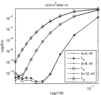
These functions have typical decay properties. The errors corresponding to the first case ( and norms respectively) are reported in Fig. 1. It is fairly clear the the accuracy depends on the scaling factor . Whenever this factor is properly chosen, even for moderate values of , the method produces results with spectral accuracy.
The presence of an oscillation factor worse considerable the approximation and requires a larger interval. The situation corresponding to the second example is summarized in Fig. 2.
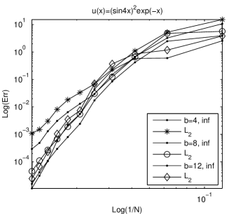
Two important conclusions can be formulated. First, in our boundary layer type problems we expect an exponential decay without oscillations of solutions. Thus the spectral accuracy can be altered only by nonlinearity of the problem. Second, for oscillatory decaying solutions, mapping techniques or even truncation domain methods can be a serious concurrent for Laguerre collocation. In Shen1 , and partially in Shen , the authors study the accuracy of Galerkin method applied to a self adjoint second order elliptic problem with similar conclusions.
3 Laguerre collocation formulation for Falkner-Skan problem
3.1 Falkner-Skan equations
The Prandtl’s boundary layer equations for flow past a flat plate in a nonuniform external flow (see for instance OO or PSDH ) reduce to the nonlinear differential equation
| (7) |
where is a real parameter, the so called Hartree parameter, and stands for the velocity inside the boundary layer. This is known as the Falkner-Skan equation. In fact signifies the dimensionless pressure gradient parameter and where comes from the expression of the free stream velocity , being a real constant.
The viscous boundary conditions reduces themselves to the following three
| (8) |
Whenever there exists heat transfer between the wall and viscous incompressible fluid moving along, the energy equation reduces to the nonlinear second order equation (see for instance RVV )
| (9) |
where stands for nondimensional temperature and for Prandtl number. The equation (9) is supplied with the following two boundary conditions
| (10) |
As soon as the problem (7)-(8) is solved, the problem (9)-(10) becomes linear and immediately solvable. The left hand side part of (7) is also present in the boundary layer equations of two-dimensional laminar and turbulent flows (see for instance CS ).
3.2 The Laguerre differentiation matrices
In order to solve the two-point boundary value problem (12) by Laguerre collocation we represent by the interpolate defined by
| (14) |
where are the cardinal Lagrangian interpolating polynomials
| (15) |
The interpolating nodes , are the first roots of Laguerre polynomials and we add a node in order to facilitate the incorporation of boundary conditions. The interval can be mapped to itself by change of variables where is any positive real number (the scaling factor). Laguerre method therefore contains a free-parameter. It means that the Laguerre interpolating process is exact for functions of the form
| (16) |
where is any polynomial of degree or less.
In order to write down the Laguerre collocation equations for (12) we use the Laguerre differentiation matrices from the paper of Weideman and Reddy WR (see also F ). Let us denote these matrices by where is the differentiation order.
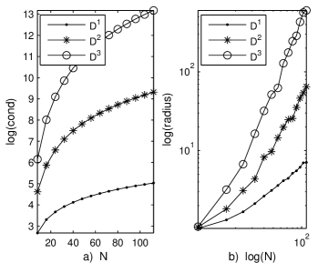
Unfortunately, these matrices are fully populated, non symmetric and quite bad conditioned. In Fig. 3 we report the dependence of their conditioning on and the dependence of their spectral radius on the same cut off parameter. Anyway, a simple comparison with our results reported in CIGIFD shows better conditioned Laguerre differentiation matrices than Chebyshev counterpart. With respect to the spectral radius we observe that they are of order and for the first, second and respectively third differentiation matrices.
This aspect is the main disadvantage of spectral collocation methods when compared with spectral Galerkin.
3.3 The Laguerre collocation algorithm
Boundary conditions
With respect to the boundary conditions, both classes of problems at hand contain behavioral, i.e., at infinity as well as numerical, i.e., in the origin, boundary conditions (see Boyd JPB for this classification). The boundary conditions at infinity are directly satisfied by Laguerre functions. In fact we have
| (17) |
for any natural number .
The conditions at zero are introduced by a removing technique of independent boundary conditions due to J. Hoepffner JH . In a few words, we consider the boundary conditions on the origin as two linear constraints on the state of our system of degrees of freedom and remove them since they are slaved to the other degrees which we keep. Thus, we decompose the state in degrees of freedom that we keep and degrees of freedom that we remove. We express the removed state variables as a function of the kept ones, thus preserving their action in the system. Moreover, we are not interested in the evolution of the removed degrees of freedom since we can, at any time, recover them from the kept ones.
A fairly similar technique is used in WR where the authors introduce some hinged boundary conditions in a fourth order problem.
This simple and efficient algorithm in imposing the boundary conditions in collocation methods is a serious advantage when compare with Galerkin methods.
The equations of Laguerre collocation
The method casts the problem (12) into the following nonlinear algebraic system
| (18) |
In (18) the vector contains the nodal unknown values , i.e., the kept degrees of freedom from . The tilde placed over differentiation matrices means that the first two rows and columns of these matrices are deleted and the Dirichlet and Neumann boundary conditions on zero were already incorporated using a constraint matrix. The matrices are diagonal matrices with the diagonal entries and , respectively, and is the vector with the components
| (19) |
The MATLAB operators are used throughout this paper and thus the elementwise power of a vector is denoted by . The nonlinear algebraic system (18) was successfully solved by MATLAB built in function fsolve.
Recovering derivatives
Thus, we first get , and then, using the give-back matrix we compute and successively and The equation (11) produces the solution of the original problem. On the accuracy of this recovering process we will elaborate more in the next Section.
4 Numerical solutions to Falkner-Skan problem
A non trivial test of accuracy
First, we want to test the accuracy of our algorithm for nonlinear problem (7)-(8). This can be accomplished upon introducing a modified source term in the r. h. s. of (12) such that this problem admits the exact solution . The result of integration for and was exact to precision of order . As this error persists for vanishing and non vanishing we can asses that the nonlinearity is overwhelming responsible for this loss of accuracy comparing with . An explanation can consists in worse conditioning of the second matrix derivative with respect to the first one. We have also to mention that solving the nonlinear algebraic systems throughout this paper, the procedure was convergent in each and every situation.
Falkner-Skan and Blasius problems
The problem (7)-(8) with is the so called Blasius problem. The curves , with physical meaning of mean tangential velocity as a function of normal distance, and are depicted in Fig. 4.
The value of the second derivative , which physically means the drag on the flat plate was found to be This value is larger than reported in Ro or reported in RVV . Both results were obtained making use of shooting and domain truncation. With respect to our numerical results we have to observe that very close to the flat plate the recovered values of the second derivative display a sort of numerical instability. A reason for this inconvenience can be the lack of a boundary condition for this derivative and the round off errors which affects the second order differentiation matrix. However, with a cubic smoothing spline process from spline toolbox of MATLAB, the first two noisy values can be removed and replaced by physically reasonable values. This smoothing process is numerically stable with respect to , i.e., and scaling factor in the range
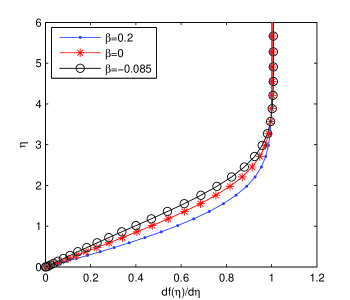
However, the mean velocity profile in Fig. 5, for positive (accelerating boundary layer flow) and negative (decelerating boundary layer flow), show excellent agreement with existing results in literature (see for instance HS , OO , Ro and PSDH ). If , so that the main stream is decreasing with respect to the longitudinal coordinate, there are two solutions of Falkner-Skan problem, provided that is not less than . One solution has a velocity profile of the normal ’kind’, i.e., , and the other has a region of reversed flow near the flat plate. The discussion of the non-existence for under this threshold is available in Rosenhead Ro (see also Acheson Ach ). In our numerical experiments, for the same initial guess, i.e. equals , we have obtained all normal ’kind’ solutions in Fig. 5.
5 Laguerre collocation solutions to Ekman layer problem
5.1 Ekman boundary layer equations
In AB the authors consider the following generalized eigenvalue problem
| (20) |
where , supplied with the boundary conditions
| (21) |
If is set equal to unity, the Rossby number equals the Reynolds number and these equations reduce exactly to those of Lilly DKL . Here is the wave number, and are two known and smooth functions and is the complex phase speed. The equations (20)-(21) define an eigenvalue problem which determine in terms of , and .
Greenberg and Marletta carried out a detailed analysis in GM , of this particular case, from operator theory point of view. They locate the essential spectrum and analyze the solutions of a related system of first order differential equations. Eventually, by domain truncation and shooting they solved numerically this system. Melander in MVM shows that this linear stability problem can be treated as an optimization problem.
One important remark is now appropriate. The system (20)-(21) can be transformed into a first order differential system of six equations as in AB or GM . The converse statement is also true, i.e. eliminating for instance variable, the system can be cast into a sixth order differential equation. As the algebraic manipulations in the general case are tedious, we consider only the case when . In this case we get the polynomial eigenvalue problem
| (22) |
with boundary conditions depending on the spectral parameter. Unfortunately, from computational point of view this formulation does not open feasible perspectives.
5.2 Laguerre collocation solutions
Rather than reproduce all the results of Lilly DKL or Allen and Bridges AB , etc., we just consider one example from these papers, namely the flow profiles:
| (23) |
The dependence of the leftmost eigenvalue on the small parameter , the Reynolds number and , is actually studied for the following discretization of the problem (20)-(21):
| (24) |
In this GEP, and being vectors of dimension and
| (25) |
The matrices are the differentiation matrices with the boundary conditions (21) introduced as in Sect. 3.2 . Along with the pencil above, we will study the pencil which provides surprising information for the spectrum of GEP (24). The matrix reads:
| (26) |
and is obtained from making .
Melander in his paper MVM solves GEP (24) as an optimization problem and finds that for the values of parameters
| (27) |
the corresponding eigenvalue has a vanishing imaginary part and the real part equals For the same values of the above parameters, the leftmost eigenvalue we have obtained reads
| (28) |
when the problem (24) was solved with and . In fact, we have obtained values of the leftmost which are indistinguishable up to the sixth digit, for in the range and scaling factor in the range . This means numerical stability of our numerical process. These numerical result are also in reasonable agreement with those published in AB , IBT and DKL .
In order to find the entire spectrum of the GEP we have used the eig MATLAB code which implements the well known QZ algorithm. The accuracy of a limited number of eigenvalues from the leftmost region of this spectrum was validated using the Jacobi-Davidson algorithm (see NR and the codes from SG ).
In order to verify the theoretical results from GM we displayed the left part of the spectrum of the unperturbed symmetric pencil and of the spectrum of for values of parameters in (27) in Fig. 6.
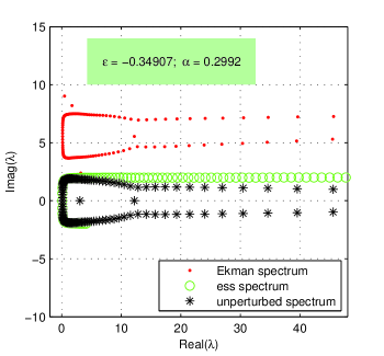
The essential spectrum is indeed contained inside the curve given parametrically by
| (29) |
where is a real parameter and the imaginary unit. The curve is marked with circles on Fig. 6.
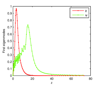
The spectrum of the GEP (24) appears to be a slightly perturbation of the symmetric spectrum of , i.e., the rightmost part is distorted and three ’rebel’ eigenvalues emerge. More than that, with Theorem 5.1 in GM , the authors show that the essential spectrum and the spectrum of the Ekman problem locate in a semi-infinite strip. Denoting this theorem predicts, in the case at hand, that and Our numerical results infer that these bounds overestimate the real situation. The first eigenmodes are depicted in Fig.7. They behave correctly at the ends of integration interval.
.
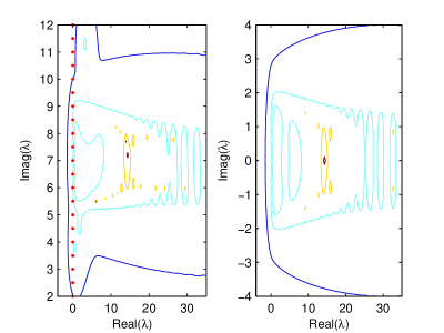
We have also computed numerically the pseudospectrum of (24) for the values (27) of parameters and . It is reported in Fig. 8 and suggests that the pencil in this marginal case is non-normal (see for instance HP for non-normality of a GEP).
6 Concluding remarks
We have introduced a general applicable Laguerre collocation type method in order to discretize high order differential equations on the half line. The method handles efficiently any type of boundary conditions and avoids the domain truncation. Moreover it has provided accurate solutions inside the boundary layer as well as in characterizing the linear hydrodynamic stability of Ekman layer. With a simple smoothing process the second derivative of the unknown in the Falkner-Skan equation is correctly recovered on a fine grid clustered toward the fixed boundary.
The method proved to be stable with respect to the order of discretization and scaling factor.
However, a systematic quantitative comparison between our numerical results and the results already obtained, mainly with shooting and truncation, is rather difficult to be carried out because our method is conceptually different.
Qualitatively, the result are similar with the older ones in both cases, a third order nonlinear boundary value problem and a fourth order eigenvalue one. However, the method is directly and easy implementable and, at least in the case of eigenvalue problems, confirm the sharpest theoretical results available, based on the operator theory. More than that, using the notion of pseudospectrum it indicates possible limitations of the linear stability analysis.
References
- (1) Acheson, D.J.: Elementary Fluid Dynamics. Clarendon Press, Oxford(1992)
- (2) Allen, L., Bridges, T.J.: Hydrodynamic stability of the Ekman boundary layer including interaction with a compliant surface: a numerical framework. Eur. J. Mech. B Fluids 22, 239-258(2003)
- (3) Bernardy, C., Maday, Y.: Spectral Methods. In Ciarlet P., Lions L., (eds) Handbook of Numerical Analysis, V.5 (Part 2), North-Holland(1997)
- (4) Boyd, J.P.: Chebyshev and Fourier Spectral Methods. Second Ed., Dover Publications, New York(2000)
- (5) Boyd,J.P., Rangan, C., Bucksbaum, P.H.: Pseudospectral methods on a semi-infinite interval with application to the hydrogen atom: a comparison of the mapped Fourier sine method with Laguerre series and rational Chebyshev expansions, J. Comp. Phys. 188, 56-74(2003)
- (6) Cebeci, T., Cousteix, J.: Modeling and Computation of Boundary Layer Flows. Horizons Publishing: Long Beach, CA and Springer-Verlag, Heidelberg(1998)
- (7) Cebeci, T., Shao, J.P.: A non-iterative method for boundary-layer equations- Part II: Two-dimensional laminar and turbulent flows. Int. J. Numer. Meth. Fluids (2003). doi: 10.1002/fld.560
- (8) Fang, T., Zhang, J.: An exact analytical solution of the Falkner-Skan equation with mass transfer and wall stretching,. Int. J. Nonlinear Mech. 43, 1000-1006(2008)
- (9) Funaro, D.: Polynomial Approximation for Differential Problems. Springer-Verlag, Berlin Heidelberg(1992)
- (10) Gheorghiu, C.I., Dragomirescu, I.F.: Spectral methods in linear stability. Application to thermal convection with variable gravity field. Appl. Numer. Math. (2009).doi:10.1016/j.apnum.2008.07.004.
- (11) Greenberg, L., Marletta, M.: The Ekman flow and related problems: spectral theory and numerical analysis. Math. Proc. Camb. Phil. Soc. 136, 719-764(2004)
- (12) Hochstenbach, M.E., Plestenjak, B.: Backward errors, condition numbers, and pseudospectra for the multiparameter eigenvalue problems. Linear Algebra Appl. 375, 63-81(2003)
- (13) Hoepffner, J.: Implementation of boundary conditions. http://www.lmm.jussieu.fr/hoepffner/research/realizing.pdf(2010). Accessed 25 August 2011
- (14) Ioss, G., Bruun, H.: True, Bifurcation of the stationary Ekman flow into a stable periodic flow. Arch. Rat. Mech. Anal. 68, 227-256(1978)
- (15) Keller, H.B.: Numerical Methods for Two-Point Boundary-Value Problems. Blaisdell Publishing Co., New-York(1968)
- (16) Lilly,D.K.: On the Instability of Ekman Boundary Flow. J. Atmospheric Sci. 23, 481-494(1966)
- (17) Melander, M.V.: An algorithmic approach to the linear stability of the Ekman layer, J. Fluid Mech. 132, 283-293(1983)
- (18) Motsa, S.S., Sibanda, P.: An efficient numerical method for solving Falkner-Skan boundary layer flows. Int. J. Numer. Meth. Fluids (2011). doi: 10.1002/fld.2570
- (19) van Noorden, T., Rommes, J.: Computing a partial generalized real Schur form using the Jacobi-Davidson method. Numer. Linear Algebra Appl. (2007). doi: 10.1002/nla.523
- (20) Ockendon, H., Ockendon, J.R.: Viscous Flow. Cambridge University Press, Cambridge(1995)
- (21) Parand, K., Dehghan, M., Pirkhedri, A.: Sinc-collocation methods for solving the Blasius equation. Phys. Letters A 373, 1237-1244(2009)
- (22) Parand, K., Dehghan, M., Pirkhedri, A.: The use of Sinc-collocation method for solving Falkner–Skan boundary-layer equation, Int. J. Numer. Meth. Fluids (2010) doi: 10.1002/fld.2493
- (23) Riley, N., Weidman, P.D.: Multiple solutions of the Falkner-Skan equation past a stretching boundary. SIAM J. Appl. Math. 49, 1350-1358(1989)
- (24) Rosales-Vera, M., Valencia, A.: Solutions of Falkner-Skan equation with heat transfer by Fourier series. Int. Comm. Heat Mass Transf. 37, 761-765(2010)
- (25) Rosenhead, L.: (Ed.) Laminar boundary layers, Clarendon Press, Oxford(1963) (Paperback edn: Dover New York, 1988)
- (26) Sachdev, P.L., Kudenatti, R.B., Bujurke, N.M.: Exact analytic solution of a boundary value problem for the Falkner-Skan equation. Stud. Appl. Math. 120, 1-16(2008)
- (27) Schlichting, H.: Boundary layer theory. Fourth Ed. McGraw-Hill (1960)
- (28) Schmid, P.J., Henningson, D.S.: Stability and Transition in Shear Flows. Springer-Verlag, New York(2001)
- (29) Shen, J.: Stable and efficient spectral methods in unbounded domains using Laguerre functions, SIAM J. Numer. Anal. 38, 1113-1133(2000)
- (30) Shen, J., Wang, L-L.: Some Recent Advances on Spectral Methods for Unbounded Domains. Commun. Comput. Phys. 5, 195-241(2009)
- (31) Shen, J., Tang, T., Wang, L-L.: Spectral Methods. Algorithms, Analysis and Applications. Springer-Verlag, Berlin Heidelberg(2011)
- (32) Sleijpen, G.L.G. Jdqz. http://www.math.uu.nl/people/sleijpen/JD_software/JDQZ.html (2004/02/05). Accessed 20 November 2011
- (33) Trefethen, L.N., Trefethen, A.E., Reddy, S.C., Discroll, T.A.: Hydrodynamic Stability Without Eigenvalues. Science 261,578-584(1993)
- (34) Trefethen, L.N.: Computation of pseudospectra. Acta Numer. 8, 247-295(1999)
- (35) J.A.C. Weideman, J.A.C., Reddy, S.C.: A MATLAB Differentiation Matrix Suite, ACM T. Math. Software 26, 465-519(2000)