Abstract
The Gaussian white noise modulated in amplitude is defined as the product of a Gaussian white noise and a slowly varying signal with strictly positive values, called volatility. It is a special case of the superstatistical systems with the amplitude as the single parameter associated to the environment variations. If the volatility is deterministic, then the demodulation, i.e., the separation of the two components from a measured time series, can be achieved by a moving average with the averaging window length optimized by the condition that the absolute values of the estimated white noise are uncorrelated. Using Monte Carlo experiments we show that the large scale deterministic volatility can be accurately numerically determined. The artificial deterministic volatilities have a variety of shapes comparable with those occurring in real financial time series. Applied to the daily returns of the S&P500 index, the demodulation algorithm indicates that the most part of the financial volatility is deterministic.
Authors
Keywords
Statistical and Nonlinear Physics; computational methods; superstatistics; volatility; artificial time series; Monte Carlo methods
Paper coordinates
C. Vamoş, M. Crăciun, Numerical demodulation of a Gaussian white noise modulated in amplitude by a deterministic volatility, Eur. Phys. J. B (2013) 86: 166.
10.1140/epjb/e2013-31072-x
References
see the expansion block below.
About this paper
Print ISSN
1434-6028
Online ISSN
1434-6036
Google Scholar
soon
Numerical demodulation of a Gaussian white noise modulated in amplitude by a deterministic volatility
“T. Popoviciu” Institute of Numerical Analysis,Romanian Academy,
P.O. Box 68, 400110 Cluj-Napoca, Romania
Abstract
The Gaussian white noise modulated in amplitude is defined as the product of a Gaussian white noise and a slowly varying signal with strictly positive values, called volatility. It is a special case of the superstatistical systems with the amplitude as the single parameter associated to the environment variations. If the volatility is deterministic, then the demodulation, i.e., the separation of the two components from a measured time series, can be achieved by a moving average with the averaging window length optimized by the condition that the absolute values of the estimated white noise are uncorrelated. Using Monte Carlo experiments we show that the large scale deterministic volatility can be accurately numerically determined. The artificial deterministic volatilities have a variety of shapes comparable with those occurring in real financial time series. Applied to the daily returns of the S&P500 index, the demodulation algorithm indicates that the most part of the financial volatility is deterministic.
PACS:
05.10.Ln – Monte Carlo methods;05.45.Tp – Time series analysis;
89.65.Gh – Economics; econophysics, financial markets, business and management
1 Introduction
Many mathematical models of the financial returns time series are based on the heteroskedastic decomposition
| (1) |
where is a white noise with zero mean and unit variance, is a positive volatility time series, and the two factors are mutually independent taylor07 ; hamilton ; voit05 . But the nature of the volatility is still under debate. The dominant approach in quantitative finance is to consider the volatility as a stationary time series and to impose various explicit causal dependencies to the volatility stochastic process. The ARCH and GARCH family of models assumes parametric relations between the returns conditional variance and the history of the returns and their variances engle95 . The stochastic volatility models consider that the volatility depends on an additional white noise, besides that related to returns taylor07 . These parametric models have the tendency to become more and more complex in order to account all the features of the actual returns known as stylized facts cont01 .
In the last decade an alternative approach has been revived which considers that the volatility is not a stochastic process, but a slowly deterministic function of time. A review of the volatility estimation methods based on the local stationarity of the returns is provided in bellegem11 . There are two approaches: one is based on the definition of the locally stationary processes given by dahlhaus12 , the other assumes that the volatility is piece-wise constant davies2012 ; mercurio2004 . A more complex hypothesis is made by the spline-GARCH model for which the volatility is a superposition of a deterministic function and a stationary stochastic process engle08 .
When the volatility is deterministic, the heteroskedastic time series (1) is similar to a harmonic carrier modulated in amplitude and we call it modulated white noise. Because the deterministic volatility has a significantly slower variation than the noise fluctuations, simple numerical methods can be used to estimate the volatility, i.e., to demodulate the time series . In this paper we analyze a demodulation algorithm based on the moving average of the absolute values of the returns vamoscraciun2010 , a variant of the so-called realized volatility poon05 . Our algorithm uses no information regarding the dynamical origins of the deterministic volatility.
By Monte Carlo experiments on numerically generated time series we show that the slowly varying deterministic volatility can be accurately numerically determined. We generate the artificial volatility by a linear transformation of the trends generated by the numerical algorithm presented in vamos08 ; vamoscraciun2012 . In this way we obtain volatilities with a variety of shapes comparable with those occurring in real financial time series. The demodulation is achieved by an automatic form of the numerical algorithm presented in vamoscraciun2010 . The Monte Carlo experiments show that the demodulation algorithm can successfully estimate the deterministic volatility. Its accuracy improves when both the length of the time series and the amplitude of the volatility variations increase.
Using a minimal set of assumptions on the correlations between the two factors in Eq. (1), an elegant nonparametric test for the nature of the noise factor has been designed alfarano2008 ; wagner2010 . The results indicate that it is Gaussian for financial indices and is a superposition of a Gausian white noise (GWN) and a Laplacian white noise for individual stocks. Because our demodulation algorithm does not depend on the features of the noise factor, we use a GWN to generate the artificial returns time series. In this way we can evaluate the demodulation accuracy by verifying the normality of the estimated white noise. This assumption is also in agreement with the well-known fact that the daily residuals determined from high-frequency data have a normal distribution andersen01 .
We have applied the demodulation algorithm to the daily returns of the S&P500 index because for this time series there is evidence that it is the product of a deterministic piece-wise constant volatility and a GWN starica05 . The noise estimated by our algorithm is much closer to normality than the initial returns, however, unlike the estimated noise for the artificial time series, in this case a detectable departure from normality remains. Hence, the large scale deterministic volatility is only a first approximation of the volatility of the financial time series, a part of the real volatility having fluctuations of smaller time scales and probably of a stochastic nature.
The modulated GWN is a special case of the time series describing superstatistical systems characterized by a superposition of several statistics on different time scales beck03 ; beck11 . In general the superposition is controlled by one or more parameters describing the large scale variations of the environment. In case of the time series defined by Eq. (1) the volatility is the single parameter related to the environment. Many complex systems in various areas of science can be effectively approximated by a superstatistical distribution: turbulence, astrophysics, quantitative finance, climatology, random networks, medicine etc. beck09 . It has also been proved that the superstatistical model allows a structural foundation for non-Boltzmann statistical mechanics, including the Tsallis formulation hanel11 .
In the next two sections we present the algorithm to generate the artificial time series and then the demodulation algorithm. In Sec. 4 we test the algorithm on numerically generated time series, while in Sec. 5 we apply it on the daily returns of the S&P500 index and we show that the estimated white noise has a probability distribution function (pdf) much closer to a Gaussian than that of the initial returns. In the end we present some conclusions.
2 Artificial deterministic volatility
Any algorithm for volatility estimation has to be evaluated on artificial time-series for which the real volatility is known. Usually, the artificial deterministic volatility has a very simple shape, for instance, a rectangular function with two change points of the volatility mercurio2004 ; spokoiny2009 ; bellegem08 . We test our demodulation algorithm on volatilities with a variety of shapes comparable to those encountered in practice. They are derived from trends generated by the numerical algorithm presented in vamos08 ; vamoscraciun2012 .
Unlike trends, volatility is always positive. Hence any trend can be changed into a volatility time series by a linear transformation. If and are the chosen volatility extrema, then
where and are the extrema of the trend. Obviously, the adimensional parameter describing the volatility variability is the modulation ratio
Hence we characterize an artificial volatility only by the value of and we fix the volatility minimum .
The trend is constructed by joining together monotonic semiperiods of sinusoid with random amplitude vamos08 ; vamoscraciun2012 . The length of each sinusoidal segment is also random and larger than a fixed value . The orientation of the sinusoidal segments is random, but they are joined together such that the final trend should be continuous. Each segment may be increasing or decreasing with the same probability. For this reason the number of monotonic parts of the generated trend is generally less than . Finally the mean of the trend is removed from it. Hence the artificial volatility is characterized by four parameters: the length of the time series , the number of sinusoidal segments , the minimum number of volatility values in a segment , and the modulation ratio .
We choose the values of these parameters such that the artificial volatility models the large scale variations of the volatility of the daily financial returns. If are the daily prices of a financial asset, then the daily returns are defined as and they have the structure given by Eq. (1). Even if the volatility has a stochastic component, its large scale variations in a particular time series can be described by a deterministic function. For instance, the characteristic time longer than one year of the economic cycles is identified as the monotonic parts of trends in financial time series schump39 .
The length of our artificial time series varies between and around an average value of 2000 that corresponds to a period of 8 years, i.e., a period of time large enough to contain at least a global economic cycle. The number of sinusoidal segments of the artificial volatility is and it corresponds in average to 8 monotonic parts. Then, depending on the length of the time series, the average length of monotonic parts varies from several months to several years. We choose , limiting in this way the minimum length of a monotonic part to a month. The modulation ratio varies with one order of magnitude from to . With these values for the parameters , , and we obtain a large enough variability of the volatility shapes.
We multiply the artificial volatility with a GWN obtaining an artificial time series of daily returns. The mutual independence of the two factors in Eq. (1) indicates that they are generated by two distinct phenomena. While the white noise might describe a featureless background, the slowly varying amplitude is related to a greater scale phenomenon influencing the amplitude of the background fluctuations.
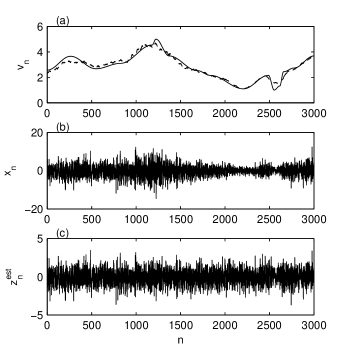
Figures 1(a) and (b) show an artificial volatility with , , , and and the corresponding modulated GWN. Such artificial time series are of the same type as the time-modulated GWN defined by bellegem04 for which in Eq. (1) is a deterministic time-varying function. It is a simple form of the locally stationary processes dahlhaus12 which have many applications in financial time series analysis bellegem11 .
3 Demodulation algorithm
There are many different algorithms for numerical demodulation of a modulated GWN. Because the volatility in Eq. (1) is slowly varying, the majority are based on stationarity tests which allow one to determine the segments of the modulated time series that can be approximated by a GWN with constant amplitude bellegem11 ; dahlhaus12 ; davies2012 ; starica05 . The demodulation algorithms applied to superstatistical time series are also obtained by segmentation in stationary parts straet09 ; gerig09 . We proposed a demodulation method based on a moving average with the length of its averaging window optimized such that the absolute values of the estimated white noise are uncorrelated vamoscraciun2010 . It is a modified form of the moving average used in liu99 and it is based on averaging historical values of the absolute or squared returns poon05 .
If is the semilength of the averaging window, then for we define the moving average
| (2) |
If (), then the average is taken over the first (the last ) values of . This asymmetric average forces the values near the time series boundaries to follow the variations of the interior values vamoscraciun2012 . If we consider as a volatility estimator, then from Eq. (1) it follows that the estimator of the white noise is
| (3) |
We have to find the optimum value for which the best approximation of the volatility is obtained.
We use the uncorrelation property of the white noise in Eq. (1). The white noise has zero mean and is uncorrelated . Its absolute values have a nonvanishing mean but they are also uncorrelated
because . Hence the optimum averaging window is obtained when the time series has a minimum serial correlation. We quantify the serial correlation by means of the sample autocorrelation function (ACF). For an infinite time series the ACF is identical zero, but we have to analyze finite time series.
For independent and identically distributed (i.i.d.) time series Bartlett’s theorem states that the values of the sample autocorrelation function asymptotically form a normal i.i.d. time series with mean zero and variance brockdav96 (p. 221). Bartlett’s theorem holds for the absolute values of a GWN too vamoscraciun2012 . We compare the distribution of the sample ACF with the theoretical normal distribution. In this way we avoid the possibility that in numerical processing the sample ACF could become too small as it is possible with the usual uncorrelation tests, like the Box–Pierce test box70 .
We measure the deviation from normality of the sample ACF of the time series by the statistic used in the Kolmogorov-Smirnov test
| (4) |
where is the sample cumulative distribution function (cdf) of and is the theoretical cdf of the normal distribution with Bartlett’s parameters. The quantity is an index measuring the nonnormality of , i.e., the serial correlation of .
Because the index depends on two variables, in order to determine the optimal value we have to establish the values of for which we analyze the variation of . There is no general rule to choose the most significant part of the ACF escan09 . Therefore we start from the observation that the largest values of ACF are usually obtained for small values of the lag . In addition, if after demodulation the first values of are distributed according to Bartlett’s distribution, then all the values of do the same. Our tests indicate that in Eq. (4) we can choose .
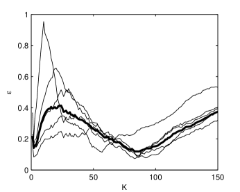
For the time series in Fig. 1(b), the variation of with respect to is represented in Fig. 2 for several values of . When has small values, the average follows closely the time series fluctuations. These fluctuations induce fluctuations of and a local minimum at small occurs. But the minimum associated to the demodulation condition is attained for larger values of which assure the removing of the small scale fluctuations from the initial time series .
The index significantly depends on (Fig. 2), therefore we eliminate this variability by averaging it with respect to In this way we obtain a function depending only on (thick line in Fig. 2) and is the value for which the minimum of occurs. For the time series in Fig. 1(b) we obtain . The estimated volatility is represented in Fig. 1(a) by a dashed line and the estimated white noise in Fig. 1(c).
The estimated volatility is smaller than the real one in the regions of the local maxima and larger near the local minima because by averaging the extrema of the volatility are attenuated. We can measure how close to the real volatility the estimated volatility is by computing the relative error
| (5) |
where is the usual quadratic norm and is the mean volatility vamos08 ; vamoscraciun2012 . For the estimated volatility in Fig. 1(a) we have . This measure of demodulation accuracy can be computed only if we know the actual volatility. An indirect method to estimate the quality of demodulation is to check the normality of the estimated white noise .
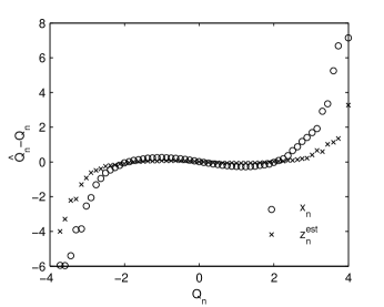
A qualitative inspection of the normality of an empirical distribution is supplied by a graph similar to the QQ plot resnick2007 . The quantile function , , is the inverse function of the cdf . If we want to verify if an observed time series is generated by an i.i.d. stochastic process with cdf equal to we graphically compare with the sample quantile function , i.e., the left-continuous inverse of the sample cdf
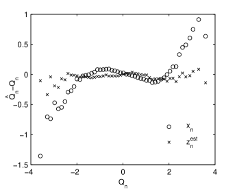
where is the indicator function of the set A. Our modified QQ plot in Fig. 3 is composed by the points with the coordinates
If the graph is close to the x-axis, then the sample distribution is the same with the theoretical distribution. The negative (positive) values of at small (large) indicate that the numerically generated time series have indeed heavy tails. Demodulation reduces these tails so that the estimated white noise has an almost Gaussian distribution.
For a quantitative estimation of normality of a time series we use the Kolmogorov-Smirnov statistic . For the estimated white noise of the time series in Fig. 1 we obtain which is half the value of the standardized initial time series , indicating the reduction of nonnormality. The kurtosis is also an indicator of the normality of a probability distribution. For the estimated white noise we have , much closer to zero (the theoretical value for a normal distribution) than the value obtained for the initial time series . This reduction of the kurtosis indicates that the heavy tails have been effectively removed by demodulation.
4 Estimation of the artificial volatility
The Monte Carlo method demands an automatic form of the demodulation algorithm. The main problem is to automatically choose the optimal value of the averaging semilength corresponding to the demodulation condition. It happens quite frequently that the minimum of the average index situated at small values of is smaller than that associated to (see Fig. 2). Therefore it is necessary to introduce a lower limit such that we search only for . If is too small, then we do not eliminate all the values of influenced by the small scale fluctuations of the returns. If is too large, then the correct value of is eliminated. Our tests indicate that an optimum value is .
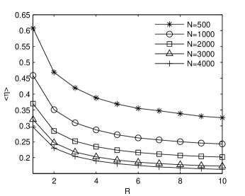
We evaluate the demodulation algorithm on statistical ensembles of 100 artificial time series and, as expected, the average relative error decreases when both and increase (Fig. 4). Hence, the longer the time series and the larger the modulation ratio, the closer the estimated volatility to the real volatility is. When the estimated volatility has a good resemblance with the real one [see Fig. 1(a)]. Large differences between them appear when . For time series with the demodulation algorithm estimates well the volatility, especially when . Even for a weak modulation (), the estimated volatility contains enough information about the real volatility. The increase of the length of the time series from to does not significantly improve the accuracy of the estimated volatility. Taking into account that by increasing the time series length, the processing time also increases, we can consider that is the optimum length for applying the demodulation algorithm for this type of time series. When , the difference between the estimated volatility and the real one becomes larger, especially for small .
In order to check if the estimated white noise is a GWN we compute the average over statistical ensembles of the Kolmogorov-Smirnov statistic , the kurtosis , and the uncorrelation index of the estimated white noise. We analyze only the time series having the optimum length . Figure 5(a) shows the average Kolmogorov-Smirnov statistic of the initial time series and of the estimated white noise . We plot with error bars the average and the standard deviation of for GWNs with the same length . For a weak modulation () the pdf of the initial time series can be confounded with a Gaussian, but for larger values of the difference significantly increases. The pdf of the estimated white noise cannot be distinguished from a Gaussian for all values of , hence the distribution of the white noise obtained by demodulation is almost Gaussian.
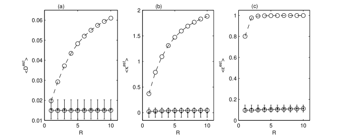
The same conclusion results from the average kurtosis [Fig. 5(b)] and from the average uncorrelation index [Fig. 5(c)]. We remark that for the initial time series with , because all the first values of are much larger than and then in Eq. (4) all the values of are close to the unit while is zero. These results prove that in average the demodulation algorithm succeeds to separate a GWN from the modulated artificial time series.
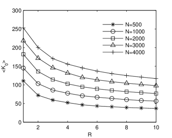
Figure 6 shows the variation of the average optimum semilength of the moving average window with respect to and . It increases when N increases and the modulation ratio decreases. As a consequence of these results we have limited the maximum value of to 350.
5 Financial volatility
We apply the modified automatic form of the demodulation algorithm to the daily returns of the S&P500 index from 3 January 1950 to 28 June 2012 plotted in Fig. 7(a) with values. To avoid squeezing the shape of the returns time series we do not plot the maximum absolute value of the returns reached on October 16, 1987.
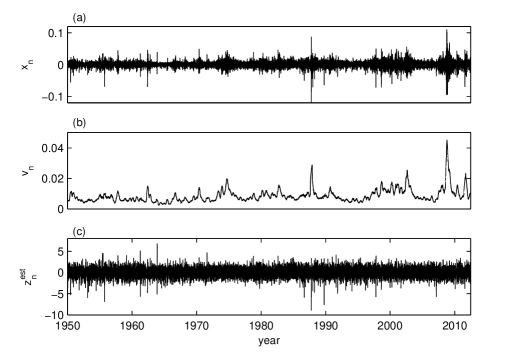
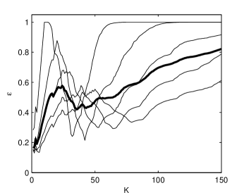
The index is represented with thin lines in Fig. 8 for several values of and their average with a thick line. We remark that has almost the same shape as that for the artificial time series in Fig. 2, but in this case the first minimum is smaller than the second one. Using the threshold value , the optimum semilength of the averaging window is the second minimum equal to . The global estimated volatility is plotted in Fig. 7(b) and the estimated white noise is represented in Fig. 7(c).
Because we do not know the real volatility, we cannot compute the index defined by Eq. (5) and the demodulation accuracy can be estimated only indirectly. The distribution of the estimated white noise is closer to that of a normal distribution than the returns distribution (Fig. 9). However, unlike the estimated white noise for the artificial time series in Fig. 3, now the heavy tails are only partially reduced, especially for negative values. We also notice that the deviation from normality for the S&P500 returns and the estimated white noise is an order of magnitude larger than for the artificial time series.
For the estimated white noise of the S&P500 returns we obtain which is three times smaller than the value of the standardized initial time series , indicating the reduction of nonnormality. The kurtosis of the estimated white noise is , much smaller than the value obtained for the initial time series . This reduction of the kurtosis indicates that the heavy tails have been significantly reduced by demodulation. We also notice that the skewness of the estimated white noise is smaller than that of standardized S&P500 returns which was .
The same conclusion results from the large value of the estimated modulation ratio for S&P500 returns. If we remove the largest 0.5% values of the returns, then the estimated modulation ratio decreases to . If we remove 1% of values, it becomes , so the large value of the estimated modulation ratio for the whole series is due only to a few extreme values.
We can evaluate the variation of the demodulation accuracy in terms of the length of the returns time series if we split the S&P500 returns into disjoint parts with equal length. We apply the demodulation algorithm separately for each part and then we compute over the parts with the same length the average of the Kolmogorov-Smirnov statistic , the kurtosis and the skewness for the returns and for the estimated white noise (Fig. 10). We compare these values with the averages and standard errors obtained for 1000 generated GWNs with the lengths equal to those of the parts in each partitioning. One notices that the averages for the estimated white noise are much closer to those for the Gaussians than those for the initial time series. However, unlike the artificial time series (Fig. 5), they do not become normally distributed.
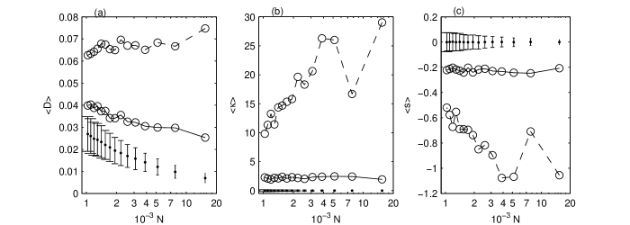
The heavy tails of the financial returns are the main cause of nonnormality as made obvious by the average kurtosis of the financial returns [Fig. 10(b)] which is one order of magnitude larger than that for the artificial time series in Fig. 5(b). In comparison with the returns kurtosis, the variation range of the Gaussian kurtosis becomes negligible and the error bars in Fig. 10(b) become almost unperceivable. Another characteristic of the financial returns is their negative skewness which is significantly reduced by demodulation [Fig. 10(c)]. Since the modulated Gaussian white noise is symmetric, this smaller skewness is also due to the reduction of the fat tails of the estimated white noise.
The extreme values of the returns and volatilities are related to the financial crisis. According to the heteroskedastic model (1), these extreme values are entirely explained by the volatility, the GRW having no heavy tails. However, because we estimate only the deterministic large scale volatility, the small scale variations of the volatility remains undetected and they manifest themselves as heavy tails of the estimated noise. For instance, the maximum absolute value of the estimated noise corresponds to the financial crisis on October 16, 1987, when the maximum absolute value of the returns also occurred (Fig. 7). But there are other financial crisis, like that on October 2008, which are completely described by the estimated volatility.
6 Conclusions
We have tested an automatic demodulation algorithm on a statistical ensemble of artificial time series with a variety of volatility shapes comparable to those encountered in real daily returns. Such Monte Carlo ensembles can be used to test any algorithm for volatility estimation. Usually artificial deterministic volatilities with much simpler shapes are considered. It is also important to remark that Monte Carlo experiments can be performed only if the demodulation algorithm has an automatic form.
The Monte Carlo experiments prove that the demodulation algorithm based on an optimized moving average can determine with accuracy the large scale deterministic volatility that modulates a Gaussian white noise. The estimated volatility approximates better the volatility for long time series with large modulation ratios. The differences between the real and the estimated volatility are of small temporal scale and originate in the volatility local extrema smoothed by the moving average. Therefore they do not affect the Gaussian distribution of the estimated white noise.
The estimated white noise obtained by demodulating the S&P500 daily returns is not Gaussian, hence the financial time series have a more complex structure than those used in our Monte Carlo experiments. However, the pdf of the estimated white noise is much closer to a Gaussian than the pdf of the initial returns, showing that the large scale deterministic volatility is a first approximation of the financial time series. Scaling properties of financial time series suggest that volatility is a superposition of correlated components of different scales mantegna95 ; Gopi99 . Hence, there are volatility components of small scales for which an improved demodulation algorithm is needed.
References
- (1) S.J.Taylor, Asset Price Dynamics, Volatility, and Prediction (Princeton University Press, Princeton, 2007)
- (2) J.D. Hamilton, Time Series Analysis (Princeton University Press, Princeton, 1994)
- (3) J. Voit, The Statistical Mechanics of Financial Markets, 3rd ed. (Springer, Berlin, 2005)
- (4) ARCH, Selected Readings edited by R.F. Engle (Oxford University Press, Oxford, 1995)
- (5) R. Cont, Quant. Financ. 1, 223 (2001) doi:10.1080/713665670
- (6) S. Van Bellegem, in Wiley Handbook in Financial Engineering and Econometrics: Volatility Models and Their Applications, edited by L. Bauwens, C. Hafner, S. Laurent (Wiley, New York, 2011) p. 323
- (7) R. Dahlhaus, in Time Series Analysis: Methods and Applications edited by T.S. Rao, S.S. Rao, C.R. Rao (North-Holland, Oxford, 2012) p. 351
- (8) L. Davies, C. Höhenrieder, W. Krämer, Comput. Stat. Data An. 56, 3623(2012) doi:10.1016/j.csda.2010.06.027
- (9) D. Mercurio, V. Spokoiny, Ann. Statist. 32, 577 (2004) doi:10.1214/009053604000000102
- (10) R.F. Engle, J.G. Rangel, Rev. Financ. Stud. 21, p. 1187 (2008) doi:10.1093/rfs/hhn004
- (11) C. Vamoş and M. Crăciun, Phys. Rev. E 81, 051125 (2010), doi:10.1103/PhysRevE.81.051125
- (12) S.-H. Poon, A Practical Guide to Forecasting Financial Market Volatility (Wiley Finance, 2005)
- (13) C. Vamoş, M. Crăciun, Phys. Rev. E 78, 036707 (2008), DOI:10.1103/PhysRevE.78.036707
- (14) C. Vamoş, M. Crăciun, Automatic Trend Estimation (Springer, Dordrecht, 2012)
- (15) S. Alfarano, F. Wagner, M. Milaković, Appl. Financial Econ. Lett. 4, 311 (2008) doi:10.1080/17446540701736010
- (16) F. Wagner, M. Milaković, S. Alfarano, Eur. Phys. J. B 73, 23 (2010) doi:10.1140/epjb/e2009-00358-1
- (17) T.G. Andersen, T. Bollerslev, F.X. Diebold, H. Ebens, J. Financ. Econ. 61, 43-76, (2001) doi:10.1016/S0304-405X(01)00055-1
- (18) C. Stărică, C. Granger, Rev. Econ. Stat. 87, 503 (2005), doi:10.1162/0034653054638274
- (19) C. Beck, E.G.D. Cohen, Physica A 322, 267 (2003) doi:10.1016/S0378-4371(03)00019-0
- (20) C. Beck, Phil. Trans. R. Soc. A 369, 453 (2011) doi:10.1098/rsta.2010.0280
- (21) C. Beck, Braz. J. Phys. 39, 357 (2009) doi:10.1590/S0103-97332009000400003
- (22) R. Hanel, S. Thurner, M. Gell-Mann, PNAS 108, 6390 (2011) doi:10.1073/pnas.1103539108
- (23) V. Spokoiny, Ann. Statist. 37, 1405 (2009) doi:10.1214/08-AOS612
- (24) S. Van Bellegem, R. von Sachs, Ann. Statist. 36, 1879 (2008) doi:10.1214/07-AOS524
- (25) J.A. Schumpeter, Business Cycles. A Theoretical, Historical and Statistical Analysis of the Capitalist Process (McGraw-Hill, New York, 1939)
- (26) S. Van Bellegem, R. von Sachs, Int. J. Forecasting 20, 611 (2004) doi:10.1016/j.ijforecast.2003.10.002
- (27) E. Van der Straeten, C. Beck, Phys. Rev. E 80, 036108 (2009) doi:10.1103/PhysRevE.80.036108
- (28) A. Gerig, J. Vicente, M.A. Fuentes, Phys. Rev. E 80, 065102 (2009) doi:10.1103/PhysRevE.80.065102
- (29) Y. Liu, P. Gopikrishnan, P. Cizeau, M. Meyer, C.-K. Peng, H.E. Stanley, Phys. Rev. E 60, 1390 (1999) doi:10.1103/PhysRevE.60.5305
- (30) P.J. Brockwell, R.A. Davies, Time Series: Theory and Methods (Springer Verlag, New York, 1996)
- (31) G.E.P. Box, D.A. Pierce, J. Am. Stat. Assoc. 65, 1509 (1970)
- (32) J.C. Escanciano and I.N. Lobato, J. Econometrics 151, 140 (2009) doi:10.1016/j.jeconom.2009.03.001
- (33) S.I. Resnick, Heavy tails Phenomena. Probabilistic and Statistical Modeling (Springer, New York, 2007)
- (34) R.N. Mantegna, H.E. Stanley, Nature 376, 46 (1995) doi:10.1038/376046a0
- (35) P. Gopikrishnan, V. Plerou, L.A. Nunes Amaral, M. Meyer, H.E. Stanley, Phys. Rev. E 60, 5305 (1999) doi:10.1103/PhysRevE.60.5305