With the scalar measure of non-normality introduced in our paper [1] we try to quantify the non-normality of three Chebyshev-type methods corresponding to differential operators involved in a second order two-point boundary value problem. To be more specific we work with Chebyshev-tau method (CT for short), a Chebyshev-Galerkin method suggested by J. Shen (CGS for short) in his paper [7],

and a Chebyshev-Galerkin method (CG for short) with different trial and test basis functions analyzed in our previous papers [5], [4], [2] and [6].

In the most significant cases we also display the corresponding pseudospectra. We want to point out the fact that, besides the pseudospectra, our scalar measure of non-normality can be thought of as a fairly reasonable characteristic of non-normality of square matrices. More, it has an important advantage. By use of this scalar measure the matrices, and consequently the numerical methods, can be compared.

In order to quantify the non-normality of the first three differential operators when they are discretized using the above mentioned methods we consider the following two-point boundary value problem:

It is well known that a matrix is non-normal if it does not commute with its conjugate transpose, i.e., $A^{\ast }A-A{A}^{\ast }\ne 0$$A^{\ast }A-A{A}^{\ast }\ne 0$A^(**)A-AA^(**)!=0A^{*} A-A A^{*} \neq 0$A^{\ast }A-A{A}^{\ast }\ne 0$ - the null matrix. We recall that for a square (non null) matrix $A$$A$AA$A$ of dimension $N$$N$NN$N$ with complex entries, its non-normality ratio, introduced in [1], reads as follows

where * stands for the conjugate transpose of $A$$A$AA$A$ and $\epsilon (A)$$\epsilon (A)$epsi(A)\varepsilon(A)$\epsilon (A)$ means the Frobenius norm of $A$$A$AA$A$. This is indeed a scalar measure (see [1]) and it satisfies the sharp inequality

For the classical CT method we refer to the well known monograph Gottlieb and Orszag [3], pp. 119-120.

For the CGS method we found out the matrices from the paper [7] P. 4.
Eventually, all the technicalities implied by CG method are available in the report of I. S. Pop [4]. For various values of parameters $\mu$$\mu$mu\mu$\mu$ and $\lambda$$\lambda$lambda\lambda$\lambda$ the non-normality ratios are displayed in the following three tables.

It is well known that the non-normality of matrices is also investigated using the notion of pseudospectrum i.e., the spectrum of the randomly perturbed matrix with an arbitrary small quantity. Up to our knowledge a direct connection between scalar measures of non-normality and pseudospectra does not exist.

For example, the pseudospectra reported in Figures 1 and 2 look very different even if they correspond to matrices with close values of non-normality ratios.

While for the CG method the spectrum contains complex eigenvalues, and the pseudospectrum underlines the spectral instability, in case of CGS method all eigenvalues are pure real and the spectral instability is almost absent. Thus, in spite of the fact that a matrix is non-normal, its pseudospectrum does not perceive this anomaly. In this situation we must resort to a scalar measure in order to observe the non-normality. We also observe that the complex part of the spectrum is much more instable than the real counterpart.

Remark 1. A Matlab code was used in order to work out the entries of Tables 1,2 and 3. The pseudospectra were depicted using a slightly modified code from the paper of L. N. Trefethen [8].

First of all, it is very clear from Tables 1 and 2 that the CT method is worse with respect to normality and its non-normality does not vary with the dimension $N$$N$NN$N$ of the approximation.

The most normal method seems to be CGS. Anyway, for large $N$$N$NN$N$ the CG and CGS methods become closer and closer. At the same time, it is quite surprising that in the absence of the first order term (see Table 3) these methods seem to converge to
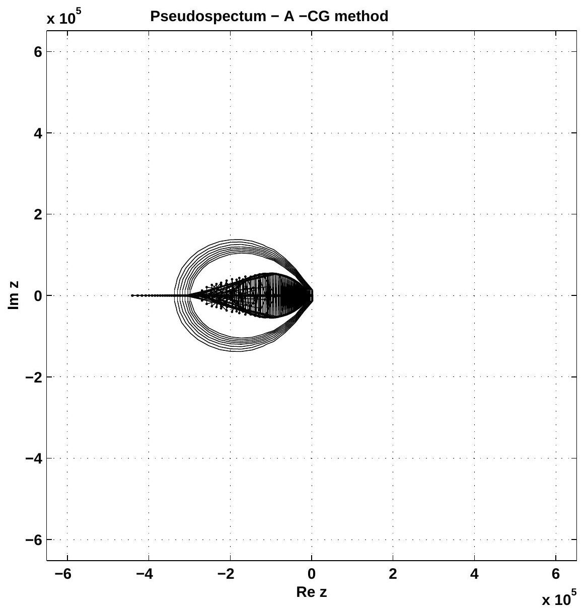
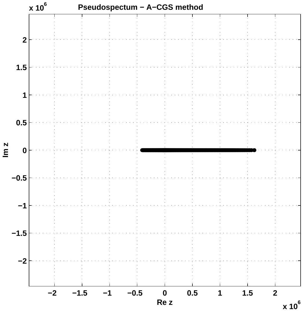
the same value of non-normality, CG decreasing and CGS increasing for large values of cutoff parameter $N$$N$NN$N$.

Finally, we have to remark that in spite of the fact that in cases considered in Figures 1 and 2 the non-normality ratios are quite closed, the pseudospectra are incomparable. It seems that in such cases the information furnished by pseudospectrum could be misleading.

[1] Gheorghiu, C. I., A new Scalar Measure on Non-normality. Application to the Characterization of some Spectral Methods, under evaluation at SIAM J. Sci. Comput.
[2] Gheorghiu, C. I., Pop, I. S., On the Chebyshev-tau Approximation for some Singularly Perturbed Two-Point Boundary Value Problems, Rev. d'Analyse Numerique et de Theorie de l'Approximation, 24(1995), 125-129.
[3] Gottlieb, D., Orszag, S. A., Numerical Analysis of Spectral Methods: Theory and Applications, SIAM Philadelphia, 1977.
[4] Pop, I. S., Numerical approximation of differential equations with spectral methods (in Romanian), Technical report, "Babes-Bolyai" University Cluj-Napoca, Faculty of Mathematics and Informatics, Cluj-Napoca, 1995.
[5] Pop, I. S., A stabilized approach for the Chebyshev-tau method, Studia Univ. "BabesBolyai", Mathematica, 42(1997), 67-79.
[6] Pop, I. S., Gheorghiu, C. I., Chebyshev-Galerkin Methods for Eigenvalue Problems, Proceedings of ICAOR, Cluj-Napoca, 1996, vol. II, 217-220.
[7] Shen, J., Efficient spectral-Galerkin method II, Direct solvers of second and fourth equations using Chebyshev polynomials, SIAM J. Sci. Stat. Comput., 16(1995), 74-87.
[8] Trefethen, L. N., Computation of Pseudospectra, Acta Numerica, 1999, 247-295.