Abstract
Transport processes in groundwater systems with spatially heterogeneous properties often exhibit anomalous behavior. Using first-order approximations in velocity fluctuations we show that anomalous superdiffusive behavior may result if velocity fields are modeled as superpositions of random space functions with correlation structures consisting of linear combinations of short-range correlations. In particular, this corresponds to the superposition of independent random velocity fields with increasing integral scales proposed as model for evolving scale heterogeneity of natural porous media [Gelhar, L. W. Water Resour. Res. 22 (1986), 135S-145S]. Monte Carlo simulations of transport in such multi-scale fields support the theoretical results and demonstrate the approach to superdiffusive behavior as the number of superposed scales increases.
Authors
Keywords
Porous media; Random fields; transport; random walk
Cite this paper as:
N. Suciu, S. Attinger, F.A. Radu, C. Vamos, J. Vanderborght, H. Vereecken, P. Knabner, Solute transport in aquifers with evolving scale heterogeneity, Analele Stiint. Univ. Ovidius C.- Mat., 23 (2015) 3, 167-186.
doi: 10.1515/auom-2015-0054
References
About this paper
Print ISSN
Not available yet.
Online ISSN
1844-0835
Google Scholar Profile
[1] Attinger, S., Dentz, M., H. Kinzelbach, and W. Kinzelbach (1999), Temporal behavior of a solute cloud in a chemically heterogeneous porous medium, J. Fluid Mech., 386, 77-104.
CrossRef (DOI)
[2] Bellin, A., M. Pannone, A. Fiori, and A. Rinaldo (1996), On transport in porous formations characterized by heterogeneity of evolving scales, Water Resour. Res., 32, 3485-3496.
CrossRef (DOI)
[3] Cintoli, S., S. P. Neuman, and V. Di Federico (2005), Generating and scaling fractional Brownian motion on finite domains, Geophys. Res. Lett. 32, L08404,
CrossRef (DOI).
[4] Dagan, G. (1994), The significance of heterogeneity of evolving scales and of anomalous diffusion to transport in porous formations, Water Resour. Res., 30, 3327-3336, 1994.
CrossRef (DOI)
[5] Dagan, G. (1987), Theory of solute transport by groundwater, Annu. Rev. Fluid Mech., 19, 183-215.
CrossRef (DOI)
[6] Dagan, G. (1988), Time-dependent macrodispersion for solute transport in anisotropic heterogeneous aquifers, Water Resour. Res., 24, 1491-1500.
CrossRef (DOI)
[7] Dentz, M., H. Kinzelbach, S. Attinger, and W. Kinzelbach (2000), Temporal behavior of a solute cloud in a heterogeneous porous medium 1. Point-like injection, Water Resour. Res., 36, 3591-3604.
CrossRef (DOI)
[8] Dentz, M., H. Kinzelbach, S. Attinger, and W. Kinzelbach (2000), Temporal behavior of a solute cloud in a heterogeneous porous medium 2. Spatially extended injection, Water Resour. Res., 36, 3605-3614.
CrossRef (DOI)
[9] Di Federico, V., and S. P. Neuman (1997), Scaling of random fields by means of truncated power variograms and associated spectra, Water Resour. Res., 33, 1075-1085.
CrossRef (DOI)
[10] Fiori, A. (1996), Finite Peclet extensions of Dagan’s solutions to transport in anisotropic heterogeneous formations, Water Resour. Res., 32, 193-198.
CrossRef (DOI)
[11] Fiori, A. (2001), On the influence of local dispersion in solute transport through formations with evolving scales of heterogeneity, Water Resour. Res., 37, 235-242.
CrossRef (DOI)
[12] Fiori, A., and G. Dagan (2000), Concentration fluctuations in aquifer transport: A rigorous first-order solution and applications, J. Contam. Hydrol., 45, 139-163.
CrossRef (DOI)
[13] Gelhar, L. W. (1986), Stochastic subsurface hydrology from theory to applications, Water Resour. Res., 22, 135S-145S.
CrossRef (DOI)
[14] Gelhar, L. W., and C. L. Axness (1983), Three-dimensional stochastic analysis of macrodispersion in aquifers, textit Water Resour. Res., 19, 161-180.
CrossRef (DOI)
[15] Gradshteyn, I. S., and I. M. Ryzhik (2007), Table of Integrals, Series, and Products, Elsevier, Amsterdam.
[16] Jeon, J.-H., and R. Metzler (2010), Fractional Brownian motion and motion governed by the fractional Langevin equation in confined geometries, Phys. Rev. E 81, 021103,
CrossRef (DOI)
[17] McLaughlin, D., and F. Ruan (2001), Macrodispersivity and large-scale hydrogeologic variability, Transp. Porous Media, 42, 133-154.
CrossRef (DOI)
[18] Papoulis, A., and S. U. Pillai (2009), Probability, Random Variables and Stochastic Processes, McGraw-Hill, New York.
[19] Radu, F. A., N. Suciu, J. Hoffmann, A. Vogel, O. Kolditz, C-H. Park, and S. Attinger (2011), Accuracy of numerical simulations of contaminant transport in heterogeneous aquifers: a comparative study, Adv. Water Resour. 34, 47–61.
CrossRef (DOI)
[20] Ross, K., and S. Attinger (2010), Temporal behaviour of a solute cloud in a fractal heterogeneous porous medium at different scales, paper presented at EGU General Assembly 2010, Vienna, Austria, 02-07 May 2010.
[21] Schwarze, H., U. Jaekel, and H. Vereecken (2001), Estimation of macrodispersivity by different approximation methods for flow and transport in randomly heterogeneous media, Transp. Porous Media, 43, 265-287.
[22] Suciu N. (2010), Spatially inhomogeneous transition probabilities as memory effects for diffusion in statistically homogeneous random velocity fields, Phys. Rev. E, 81, 056301,
CrossRef (DOI)
[23] Suciu, N. (2014), Diffusion in random velocity fields with applications to contaminant transport in groundwater, Adv. Water Resour. 69, 114–133.
CrossRef (DOI)
[24] Suciu, N., C. Vamo¸s, J. Vanderborght, H. Hardelauf, and H. Vereecken (2006), Numerical investigations on ergodicity of solute transport in heterogeneous aquifers, Water Resour. Res., 42, W04409,
CrossRef (DOI)
[25] Suciu N., C. Vamos, F. A. Radu, H. Vereecken, and P. Knabner (2009), Persistent memory of diffusing particles, Phys. Rev. E, 80, 061134,
CrossRef (DOI)
[26] Suciu, N., S. Attinger, F.A. Radu, C. Vamos, J. Vanderborght, H. Vereecken, P. Knabner (2011), Solute transport in aquifers with evolving scale heterogeneity, Preprint No. 346, Mathematics Department, Friedrich-Alexander University Erlangen-Nuremberg
(http://fauams5.am.uni-erlan-gen.de/papers/pr346.pdf).
CrossRef (DOI)
[27] Suciu, N., F.A. Radu, A. Prechtel, F. Brunner, and P. Knabner (2013), A coupled finite element-global random walk approach to advectiondominated transport in porous media with random hydraulic conductivity, J. Comput. Appl. Math. 246, 27–37.
CrossRef (DOI)
[28] Suciu, N., F.A. Radu, S. Attinger, L. Schuler, Knabner (2014), A FokkerPlanck approach for probability distributions of species concentrations transported in heterogeneous media, J. Comput. Appl. Math., in press,
CrossRef (DOI)
[29] Vamos, C., N. Suciu, H. Vereecken, J. Vanderborght, and O. Nitzsche (2001), Path decomposition of discrete effective diffusion coefficient, Internal Report ICG-IV. 00501, Research Center Jülich.
[30] Vamos, C., N. Suciu, and H. Vereecken (2003), Generalized random walk algorithm for the numerical modeling of complex diffusion processes, J. Comput. Phys., 186, 527-544,
CrossRef (DOI)
[31] Vanderborght, J. (2001), Concentration variance and spatial covariance in second-order stationary heterogeneous conductivity fields, Water Resour. Res., 37, 1893-1912.
CrossRef (DOI)
Paper (preprint) in HTML form
Solute transport in aquifers with evolving scale heterogeneity
Abstract
Transport processes in groundwater systems with spatially heterogeneous properties often exhibit anomalous behavior. Using first-order approximations in velocity fluctuations we show that anomalous superdiffusive behavior may result if velocity fields are modeled as superpositions of random space functions with correlation structures consisting of linear combinations of short-range correlations. In particular, this corresponds to the superposition of independent random velocity fields with increasing integral scales proposed as model for evolving scale heterogeneity of natural porous media [Gelhar, L. W. Water Resour. Res. 22 (1986), 135S-145S]. Monte Carlo simulations of transport in such multi-scale fields support the theoretical results and demonstrate the approach to superdiffusive behavior as the number of superposed scales increases.
1 Lagrangian and Eulerian representations of diffusion in random velocity fields
Let be the advection-dispersion process with a space variable drift , sample of a statistically homogeneous random
2010 Mathematics Subject Classification: Primary 76S99, 60J60; Secondary 60G60, 86A05, 82C80. Received: December, 2014.
Revised: January, 2015.
Accepted: February, 2015.
velocity field, and a local diffusion coefficient , assumed constant, described by the Itô equation
| (1) |
where is a deterministic initial position and are the components of a Wiener process of mean zero and variance .
The solution of the Fokker-Planck equation
| (2) |
which corresponds to Green’s function in Eulerian approaches to dispersion in random fields, is the density of the transition probability of the Itô process (1). Equation (2) is the starting point in Eulerian perturbation approaches .
The following three centered processes are useful to describe the effective and ensemble dispersion and the fluctuations of the center of mass: , the process centered about the mean of in single realizations of the random velocity field, , the process centered about the average of over the ensemble of realizations, , and the fluctuation of the center of mass , with . The half derivative of the variance of these tree processes defines, respectively, the effective and ensemble dispersion coefficients [1], and the center of mass coefficient [24],
| (3) |
related by .
According to (1), the process starting from verifies
| (4) |
where . The variance of the process (4) is obtained as follows,
where we used the statistical homogeneity of the velocity field, , and the independence of the Wiener process on velocity statistics, which, together, cancel the cross-correlation term. The process verifies (4) with and the second term set to zero and has the variance
Further, the definitions (3) yield
| (5) | ||||
| (6) | ||||
| (7) |
The first iteration of (4) about the un-perturbed problem consisting of diffusion with constant coefficient in the mean flow field , with trajectory , leads to replacing by in (5) and (6). Then, (5) gives the following first-order approximation of the ensemble dispersion coefficient
| (8) |
where is the Gaussian joint probability density of the process expressed with the aid of the Dirac -function [23]. Similarly, with , (6) gives the first-order approximation of the center of mass coefficient
| (9) |
Finally, is obtained from (7). Together, (7-9) give the (stochastic) Lagrangian formulation of the first-order approximation equivalent to that obtained in the Eulerian perturbation approach [1,7,8].
Remark 1. As follows from (8-9), for a superposition of statistically independent velocity fields the dispersion coefficients estimated to the first-order are given by the sum of terms determined by the corresponding correlations .
2 Quantifying anomalous diffusion by memory terms
In the following, by we denote one of the processes , or . Further, we consider the uniform time partition and for we define the increments and . For a sum of two increments we have
| (10) |
where . By iterating the binomial formula (10) one obtains:
Summing up these relations we get
| (11) |
which, using the relation
can be further expressed as
| (12) |
For , the expectation of (10) verifies
| (13) |
where . For continuous time , (13) becomes
| (14) |
According to the definition of the ensemble coefficient in (3), the half time derive of (14) yields
| (15) |
The last term of (14), is a memory term quantifying the departure from normal-diffusion behavior of the process [25,22] and its half derivative is a memory dispersion coefficient. Relations similar to (14-15) also hold for , and for . The expectation of the second term of Eq. (11),
| (16) |
is a cumulative memory term which, according to Eq. (12), contains a hierarchy of correlations between increments along paths of the transport process. Estimations of such cumulative memory terms by simulations of transport in single realizations of the random velocity field are presented in Ref. [29].
According to (15) and (5), the memory dispersion coefficient corresponding to the increment of the process over the time interval has the following Lagrangian expression
| (17) |
With (8), the first order approximation of (17) is given by
| (18) |
Memory coefficients (18) as well as their time integrals (i.e. memory terms) were computed in [25] for short range correlations of the velocity field as well as for diffusion in perfectly stratified fields (model of Matheron and de Marsily). In [22], the time behavior of the memory terms for fractional Gaussian noise has been also analyzed. Jeon and Metzler [16] used correlations of increments to quantify the memory of two special anomalous diffusion processes (fractional Brownian motion and processes governed by fractional Langevin equation). Their correlations are in fact memory terms related to the variance of the process by Eq. (13). For instance, in case of fractional Brownian motion with variance and Hurst coefficient , for two successive time intervals , from (14) one obtains
| (19) |
which is just Eq. (4.4) of Jeon and Metzler [16].
3 Explicit first-order results for transport in aquifers
Approximations of the flow and transport equations for small variance of the logarithm of the hydraulic conductivity of the aquifer system lead to explicit functional dependencies of the dispersion coefficients on the covariance of the random field [14].
With the common convention for the Fourier transform
| (20) | ||||
| (21) |
the first-order approximation in yields (e.g., [14, 21, 7,8 ])
| (22) |
where are projectors which ensure the incompressibility of the flow.
Remark 2. The Dirac function which ensures the statistical homogeneity in (22) has to be changed into to obtain a similar first-order relation for , where denotes the complex conjugate [5, 6, 21]. Even though it leads to the same results, this relation render the computation more complicated.
Using the inverse Fourier transform (21) and (22), the Eulerian velocity correlation from (8) and (18) can be computed as follows
| (23) |
With (23), the integrand of the time integral in (8) and (18) becomes
| (24) |
The passage to the last line in (24) was achieved by using the expression
of the characteristic function of the Gaussian increment of the un-perturbed process (see e.g. [18]).
Remark 3. Changing the sign convention of the Fourier transform,
changes the sign of the first term of the characteristic function without altering the sign of the second term, (see detailed computation of characteristic function for Gaussian random variables of Pa poulis and Pillai [18], Example 5-28, p. 153]. However, changing the sign of the imaginary exponent is equivalent to changing into (this also changes the sign of (see Gelhar and Axness [14], Eq. (28a)), but (24) depends only on ). Since second moments and dispersion coefficients do not depend on the sign of the mean flow, the expression (26) gives the same result irrespective of the sign of the imaginary exponent.
Inserting (24) into (8) one obtains the explicit expression of the advective contribution to the ensemble dispersion coefficient,
| (25) |
With the change of variable , (25) becomes
| (26) |
Remark 4.1. The time derivative of (26) is identical with the result of Dagan ([5], Eq. (3.14); [6], Eq. (17)), and Schwarze et al. ([21], Eq. (13)). Dagan [6] derived the result by using the changed sign in the homogeneity condition (Remark 2) and opposite Fourier transform convention (Remark 3).
Remark 4.2. The opposite Fourier transform convention and the same homogeneity condition as in (22) change into and let unchanged (see Remark 3). This is the case in the derivation of the variance
by Fiori and Dagan [12] (Eq. (14)), which is exactly the integral of (25) from above, with replaced by . Dentz et al. [7] used the same conventions as Fiori and Dagan [12], (i.e. Eqs. (16) and (25) in [7]) and obtained the same result. The result given by their Eq. (40) with replaced by the characteristic function of the un-perturbed problem ([7], Eq. (25)), is just the relation (26) from above, with exponent replaced by .
The corresponding memory coefficient is similarly obtained by inserting (24) into (18),
| (27) |
Making the change of variable in (27), we see that the ensemble memory coefficients can be computed, after a simple change of the integration limits in the time integral, with the explicit expression (26) of the advective contributions to the ensemble coefficients:
| (28) |
Remark 5. The memory coefficient (27) can also be obtained within the Eulerian approach of Dentz et al. [7] if in Eq. (18) from [8] the initial concentration is replaced by the perturbation solution for point source at time given in Eq. (26) from [7], i.e. . Then Eq. (18) from [8] gives . Further, inserting in Eq. (14) from [8] and "expanding the logarithm consistently up to second order in the fluctuations" (as described at the beginning of Sect. 3.2 of [8]), should reproduce the expression (27) of the memory coefficient .
To derive the explicit form of the effective coefficients (7) we first have to compute the center of mass coefficients (9). Similarly to (24), we obtain
| (29) |
The passage to the last line in (29) is now achieved through the expressions
of the characteristic functions of the Gaussian un-perturbed process , where we used the property pointed out in Remark 3. Inserting (29) into (9), we obtain the center of mass coefficient
| (30) |
With the change of variable (which implies ) the expression (30) of the center of mass coefficients becomes
| (31) |
The center of mass coefficients (30) and the advective contribution (26) to the ensemble dispersion coefficients determine the advective contributions to the effective coefficients according to (7):
| (32) |
Remark 6. The ensemble contribution (26) and the center of mass coefficient (30) particularize to isotropic local diffusion coefficient the general relations and , respectively, derived by Dentz et al. ([7] Eq. (47)). We also note that (30) is the time derivative of the relation (15) of Fiori and Dagan [12], which, together with Remarks 4.1 and 4.2, proves the equivalence of Eulerian expressions for the ensemble and effective dispersion coefficients of Dentz et al. [7, 8] and the Lagragian expressions derived by Fiori and Dagan [12] and by Vanderborght [31] for the corresponding variances. We note here that the Eulerian approach has the important advantage of providing first-order approximations of the concentration fields (e.g., Eq. (26) in [7], on which the derivation of the dispersion coefficients is actually based).
The memory coefficient of the center of mass is readily obtained, similarly to (28), by a change of the integration limits in the expression (31) of the center of mass dispersion coefficients:
| (33) |
Finally, the memory coefficient of the effective dispersion is obtained from the relations (32), (31), and (28),
| (34) |
Remark 7. The memory coefficients (28), (33), and (34) can be computed with the explicit expressions of the advective contribution to the ensemble dispersion coefficients (25) and of the center of mass coefficients (31) by changing the lower limit of the time integrals from 0 to .
4 Explicit first-order results for power-law correlated logK fields
The first-order results for log-K fields with finite correlation lengths can be further used to develop approaches for a superposition of scales [9, 20]. To proceed, let us consider the particular case of an isotropic power-law covariance of ,
| (35) |
where is some length scale associated with the spatial extension of the system. Power-law covariances can be constructed by integrating covariances with continuously increasing finite integral scales ([15], p. 370, expression 3.478 (1.)) by the relation
| (36) |
where and . For and , (36) yields a superposition of Gaussian covariances:
| (37) |
where
| (38) |
The integrand in (37) has the from of the Gaussian considered by Dentz et al. .
Redefining in (35) as and choosing and , one constructs a power-law covariance via (36) as a superposition of exponential covariances:
| (39) |
where
| (40) |
The integrand in (39) is the isotropic version of the exponential considered by Fiori [10] and Vanderborght [31].
Remark 8. For in either (37) or (39) one obtains the covariance of the " noise" as an integral of Gaussian or exponential covariances with continuous scale parameter . Further, by defining the covariance is simply given by integrating Gaussian covariances with respect to we get in (37) or exponential covariances with respect to in (39). This corresponds to the limit of infinite superposition of log-K fields with finite correlation scales.
By the linearity of the superposition relations (37), respectively (39), we have the general relations
| (41) |
By inserting (41) in (25), (30), and (7), we finally obtain the superposition
relations
| (42) |
According to (42), the memory coefficients (28), (33), and (34) are given by integrals with respect to of the coefficients for given derived in the previous section.
5 Numerical simulations of transport in aquifers with multiscale hydraulic conductivity
To investigate the behavior of several transport observables we conducted 256 global random walk (GRW) simulations of a two-dimensional isotropic diffusion, with coefficient which is a typical value for local dispersion coefficient in aquifers, in multiscale velocity fields. The latter, generated with the Kraichnan method, are first-order approximations of the flow equations for a field consisting of a superposition of statistically independent fields with isotropic exponential correlation and constant variance .
The integral scales (defined as integrals of the correlation function, not divided by the variance) of the fields were increased with a constant step , so that at the -the step , which results in
. For instance, the superposition of 2 fields has the variance 0.2 and the integral scale and that of seven fields (the largest one investigated here) has the variance 0.7 and .
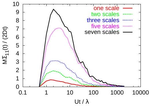
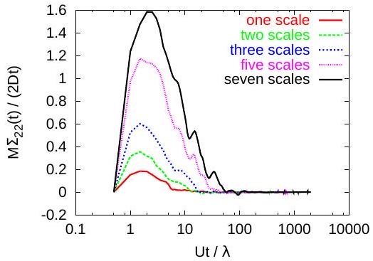
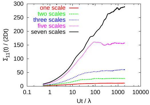
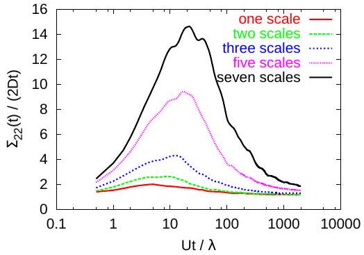
The GRW algorithm has been developed by Vamoş et al. [30]. Implementation details and applications for transport in saturated aquifers can be found in [24, 19, 27, 23, 28]. In our GRW numerical simulations we estimate dispersion coefficients for processes starting from instantaneous point injections by the mean half-slope of the variances defined in (3). The ensemble dispersion coefficients and the one-step memory dispersion coefficients , where (15), normalized by the
local dispersion coefficient, are presented in Figs. 1-4. (See Ref. [26] for results on effective and center of mass coefficients.) The extinction of the memory coefficients (Figs. 3-4) coincides with the approach to a normal diffusive behavior with constant ensemble dispersion coefficients, shown in Figs. 1-2, in agreement with (15) and (17).
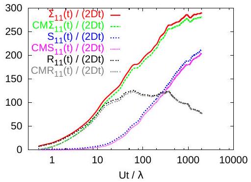
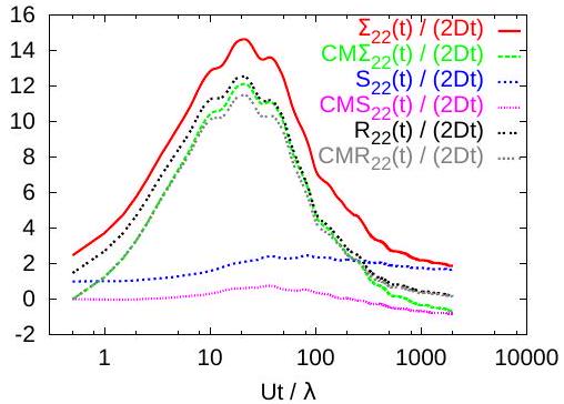
Figures 5 and 6 show the cumulative memory coefficients , with given by (16), compared with the corresponding ensemble, effective and center of mass coefficients, in case of the seven-scales velocity field. The cumulative memory coefficients are close to the corresponding dispersion coefficients, the small difference between the two coefficients being just the half slope of the average of the first term in (11). The latter is a dispersion coefficient describing the displacement of solute particles over one step (in our case, the simulation time step). In case of ensemble dispersion , we can see that the average of (11) is a discrete Taylor formula approximating the ensemble coefficient (5). Thus, ensemble coefficients are mainly determined by correlations of increments of the process , corresponding to correlations of the Lagrangian velocity. This makes the difference from genuine diffusion processes (Brownian motions) where the increments are uncorrelated and the one-step dispersion defines the constant diffusion coefficient.
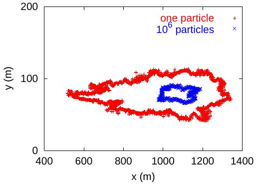
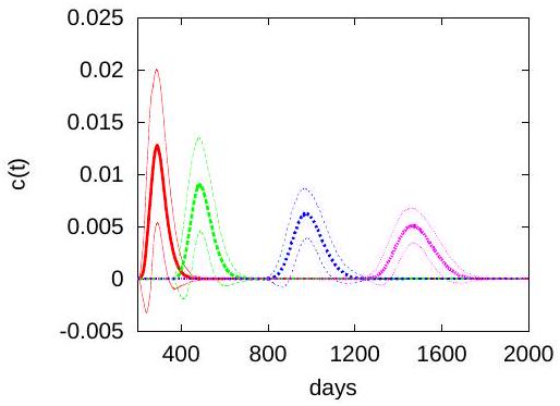
Figures 1 and 5 show that both the ensemble and the effective coefficients behave anomalous in a time windows which increase with the number of superposed scales. Anomalous diffusive behavior is also indicated by the asymmetry of the solute plume at 1000 days, presented in Fig. 7, and by the breakthrough curve of the concentration spatially averaged over the vertical section of the simulation domain, recorded at increasing distances along the mean flow direction, shown in Fig. 8. (See Ref. [26] for other simulation results which
indicate anomalous behavior).
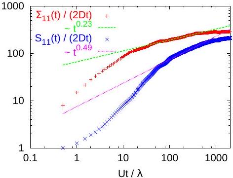
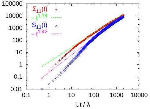
To further investigate the anomalous behavior induced by the multiscale structure of the velocity field, we fitted dispersion coefficients with power-law functions. Figures 9 and 10 indicate a power law behavior of the coefficients. We remark that ensemble and effective coefficients and variances have different time behavior, with a larger slope for the effective quantities. This seems to be at variance with the theoretical result for power-law correlated fields obtained by Fiori [11]. Therefore, we consider that the current numerical results do not allow us to draw a definite conclusion about the power law behavior of the dispersion coefficients.
As we have seen in the previous section, power-law covariances can be constructed by integrating covariances with continuously increasing integral scales. An infinite sum of equal-weight exponential correlations results in an -type correlation (Remark 8; see also expression 3.478 (1.) in [15, p. 370]) Such a correlation leads to a behavior of the ensemble variance . Since this would be the theoretical infinite limit of our simulations, we also fitted the dispersion coefficients with and the variances with (Figs. 11 and 12). At a first sight these fitting results are also acceptable. Nevertheless, a more detailed analysis is required to decide which time-behavior, the power-law one from Figs. 9-10 or the type behavior from Figs. 11-12 provides the better fit with the results of our numerical experiment. An independent selection criterium would be the numerical evaluation of dispersion and memory terms derived in Section 3 for
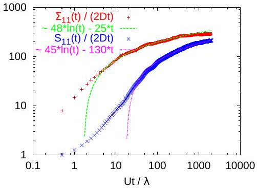
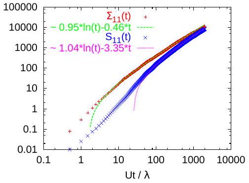
an -correlated log-K field, using the integral representation (39-40) derived in Section 4.
There is a long standing attempt to introduce power law correlations and anomalous dispersion in modeling groundwater transport by a rather abstract mathematical approach . Nevertheless, a superposition of a finite number of scales seems to be a more natural assumption in many contamination scenarios for evolving scale groundwater systems [13, 17]. Numerical simulations of transport in multiscale velocity fields provide a predictive tool for such scenarios and may support the development of adequate models.
Acknowledgements
This work was supported in part by the Deutsche ForschungsgemeinschaftGermany under Grants AT 102/7-1, KN 229/15-1, SU 415/2-1 and by the Jülich Supercomputing Centre-Germany in the frame of the Project JICG41.
References
[1] Attinger, S., Dentz, M., H. Kinzelbach, and W. Kinzelbach (1999), Temporal behavior of a solute cloud in a chemically heterogeneous porous medium, J. Fluid Mech., 386, 77-104.
[2] Bellin, A., M. Pannone, A. Fiori, and A. Rinaldo (1996), On transport in porous formations characterized by heterogeneity of evolving scales, Water Resour. Res., 32, 3485-3496.
[3] Cintoli, S., S. P. Neuman, and V. Di Federico (2005), Generating and scaling fractional Brownian motion on finite domains, Geophys. Res. Lett. 32, L08404, doi:10.1029/2005GL022608.
[4] Dagan, G. (1994), The significance of heterogeneity of evolving scales and of anomalous diffusion to transport in porous formations, Water Resour. Res., 30, 33273336, 1994.
[5] Dagan, G. (1987), Theory of solute transport by groundwater, Annu. Rev. Fluid Mech., 19, 183-215.
[6] Dagan, G. (1988), Time-dependent macrodispersion for solute transport in anisotropic heterogeneous aquifers, Water Resour. Res., 24, 1491-1500.
[7] Dentz, M., H. Kinzelbach, S. Attinger, and W. Kinzelbach (2000), Temporal behavior of a solute cloud in a heterogeneous porous medium 1. Point-like injection, Water Resour. Res., 36, 3591-3604.
[8] Dentz, M., H. Kinzelbach, S. Attinger, and W. Kinzelbach (2000), Temporal behavior of a solute cloud in a heterogeneous porous medium 2. Spatially extended injection, Water Resour. Res., 36, 3605-3614.
[9] Di Federico, V., and S. P. Neuman (1997), Scaling of random fields by means of truncated power variograms and associated spectra, Water Resour. Res., 33, 1075-1085.
[10] Fiori, A. (1996), Finite Peclet extensions of Dagan’s solutions to transport in anisotropic heterogeneous formations, Water Resour. Res., 32, 193198.
[11] Fiori, A. (2001), On the influence of local dispersion in solute transport through formations with evolving scales of heterogeneity, Water Resour. Res., 37, 235242.
[12] Fiori, A., and G. Dagan (2000), Concentration fluctuations in aquifer transport: A rigorous first-order solution and applications, J. Contam. Hydrol., 45, 139163.
[13] Gelhar, L. W. (1986), Stochastic subsurface hydrology from theory to applications, Water Resour. Res., 22, 135S-145S.
[14] Gelhar, L. W., and C. L. Axness (1983), Three-dimensional stochastic analysis of macrodispersion in aquifers, textitWater Resour. Res., 19, 161180.
[15] Gradshteyn, I. S., and I. M. Ryzhik (2007), Table of Integrals, Series, and Products, Elsevier, Amsterdam.
[16] Jeon, J.-H., and R. Metzler (2010), Fractional Brownian motion and motion governed by the fractional Langevin equation in confined geometries, Phys. Rev. E 81, 021103, doi:10.1103/PhysRevE.81.021103.
[17] McLaughlin, D., and F. Ruan (2001), Macrodispersivity and large-scale hydrogeologic variability, Transp. Porous Media, 42, 133154.
[18] Papoulis, A., and S. U. Pillai (2009), Probability, Random Variables and Stochastic Processes, McGraw-Hill, New York.
[19] Radu, F. A., N. Suciu, J. Hoffmann, A. Vogel, O. Kolditz, C-H. Park, and S. Attinger (2011), Accuracy of numerical simulations of contaminant transport in heterogeneous aquifers: a comparative study, Adv. Water Resour. 34, 47-61.
[20] Ross, K., and S. Attinger (2010), Temporal behaviour of a solute cloud in a fractal heterogeneous porous medium at different scales, paper presented at EGU General Assembly 2010, Vienna, Austria, 02-07 May 2010.
[21] Schwarze, H., U. Jaekel, and H. Vereecken (2001), Estimation of macrodispersivity by different approximation methods for flow and transport in randomly heterogeneous media, Transp. Porous Media, 43, 265287.
[22] Suciu N. (2010), Spatially inhomogeneous transition probabilities as memory effects for diffusion in statistically homogeneous random velocity fields, Phys. Rev. E, 81, 056301, doi:10.1103/PhysRevE.81.056301.
[23] Suciu, N. (2014), Diffusion in random velocity fields with applications to contaminant transport in groundwater, Adv. Water Resour. 69, 114-133.
[24] Suciu, N., C. Vamoş, J. Vanderborght, H. Hardelauf, and H. Vereecken (2006), Numerical investigations on ergodicity of solute transport in heterogeneous aquifers, Water Resour. Res., 42, W04409, doi:10.1029/2005WR004546.
[25] Suciu N., C. Vamos, F. A. Radu, H. Vereecken, and P. Knabner (2009), Persistent memory of diffusing particles,Phys. Rev. E, 80, 061134, doi:10.1103/PhysRevE.80.061134.
[26] Suciu, N., S. Attinger, F.A. Radu, C. Vamos, J. Vanderborght, H. Vereecken, P. Knabner (2011), Solute transport in aquifers with evolving scale heterogeneity, Preprint No. 346, Mathematics Department, Friedrich-Alexander University Erlangen-Nuremberg (http://fauams5.am.uni-erlan-gen.de/papers/pr346.pdf).
[27] Suciu, N., F.A. Radu, A. Prechtel, F. Brunner, and P. Knabner (2013), A coupled finite element-global random walk approach to advectiondominated transport in porous media with random hydraulic conductivity, J. Comput. Appl. Math. 246, 27-37.
[28] Suciu, N., F.A. Radu, S. Attinger, L. Schüler, Knabner (2014), A FokkerPlanck approach for probability distributions of species concentrations transported in heterogeneous media, J. Comput. Appl. Math., in press, doi:10.1016/j.cam.2015.01.030.
[29] Vamoş, C., N. Suciu, H. Vereecken, J. Vanderborght, and O. Nitzsche (2001), Path decomposition of discrete effective diffusion coecient, Internal Report ICG-IV. 00501, Research Center Jülich.
[30] Vamoş, C., N. Suciu, and H. Vereecken (2003), Generalized random walk algorithm for the numerical modeling of complex diffusion processes, . Comput. Phys., 186, 527-544, doi:10.1016/S0021-9991(03)00073-1.
[31] Vanderborght, J. (2001), Concentration variance and spatial covariance in second-order stationary heterogeneous conductivity fields, Water Resour. Res., 37, 1893-1912.
Nicolae SUCIU and Peter KNABNER,
Mathematics Department,
Friedrich-Alexander University Erlangen-Nuremberg,
Cauerstr. 11, 91058 Erlangen, Germany.
Email: {knabner, suciu}@math.fau.de
Sabine ATTINGER,
Faculty for Chemistry and Earth sciences,
University of Jena,
Burgweg 11, 07749 Jena, Germany, and
Department Computational Hydrosystems,
UFZ Centre for Environmental Research,
Permoserstrae 15 04318 Leipzig, Germany.
Email: sabine.attinger@ufz.de
Florin A. RADU,
Department of Mathematics,
University of Bergen,
Allegaten 41, 5020 Bergen, Norway.
Email: Florin.Radu@math.uib.no
Călin VAMOŞ and Nicolae SUCIU,
Tiberiu Popoviciu Institute of Numerical Analysis, Romanian Academy,
Str. Fantanele 57, 400320 Cluj-Napoca, Romania.
Email: {cvamos, nsuciu}@ictp.acad.ro
Jan VANDERBORGHT and Harry VEREECKEN, Institute of Bio- and Geosciences Agrosphere (IBG-3) Forschungszentrum Jlich IBG-3, Wilhelm-Johnen-Straße, 52428 Jlich, Germany.
Email: {J.vanderborght, h.vereecken}@fz-juelich.de