Abstract
The onset of convection in a horizontal layer of fluid heated from below in the presence of a gravity field varying across the layer is numerically investigated. The eigenvalue problem governing the linear stability of the mechanical equilibria of the fluid, in the case of free boundaries, is a sixth order differential equation with Dirichlet and hinged boundary conditions. It is transformed into a system of second order differential equations supplied only with Dirichlet boundary conditions. Then it is solved using two distinct classes of spectral methods namely, weighted residuals (Galerkin type) methods and a collocation (pseudospectral) method, both based on Chebyshev polynomials. The methods provide a fairly accurate approximation of the lower part of the spectrum without any scale resolution restriction. The Viola’s eigenvalue problem is considered as a benchmark one. A conjecture is stated for the first eigenvalue of this problem.
Authors
Călin-Ioan Gheorghiu
(Tiberiu Popoviciu Institute of Numerical Analysis, Romanian Academy)
Florica-Ioana Dragomirescu
Keywords
References
See the expanding block below.
Cite this paper as
C.I. Gheorghiu, F.-I. Dragomirescu, Spectral methods in linear stability. Applications in thermal convection with variable gravity field, Appl. Numer. Math., 59 (2009) 1290-1302
doi: 10.1016/j.apnum.2008.07.004
About this paper
Print ISSN
0168-9274
Online ISSN
Google Scholar Profile
google scholar link
Paper (preprint) in HTML form
Spectral methods in linear stability. Applications to thermal convection with variable gravity field.
Abstract
The onset of convection in a horizontal layer of fluid heated from below in the presence of a gravity field varying across the layer is numerically investigated. The eigenvalue problem governing the linear stability of the mechanical equilibria of the fluid, in the case of free boundaries, is a sixth order differential equation with Dirichlet and hinged boundary conditions. It is transformed into a system of second order differential equations supplied only with Dirichlet boundary conditions. Then it is solved using two distinct classes of spectral methods namely, weighted residuals (Galerkin type) methods and a collocation (pseudospectral) method, both based on Chebyshev polynomials. The methods provide a fairly accurate approximation of the lower part of the spectrum without any scale resolution restriction. The Viola’s eigenvalue problem is considered as a benchmark one.
MSC2000:65L10; 65L15; 65L60;76E06
Keywords: Bénard convection; variable gravity field; hydrodynamic
stability; high order two-point boundary value problem; hinged boundary
conditions; spectral methods;
1 Introduction
It is a matter of evidence that the hydrodynamic stability problems become more complex due to incorporation of technologically important effects. Consequently, the order of the differential equations increases rapidly.
Generally the discretization methods applied to such problems lead to matrices which become less conditioned as both the order of approximation and the order of differentiation increase. This fact is particularly true for spectral methods. Roughly, for ( stands for the spectral parameter), the condition number for the second order Chebyshev differentiation matrix is of order that of the fourth order differentiation matrix attains something of order and eventually that of the eighth order differentiation matrix raises to something of order
In this context, the aim of this paper is two-fold. First, we introduce a new method to solve numerically even and high order two-point boundary value problem with Dirichlet and hinged boundary conditions. It reduces the problem to a system of second order differential equations supplied only with Dirichlet boundary conditions. Further, accurate spectral methods are used in order to solve that Dirichlet boundary value problem numerically. Second, the method is applied to solve a hydrodynamic stability problem of Bénard type.
It is well known that, the classical Orr-Sommerfeld eigenvalue problem, which is encountered in the linear hydrodynamic stability analysis of some basic flows, was first solved using a direct (tau) spectral method by S. Orszag in 1971 in his seminal paper [21]. He determined the critical Reynolds number associated with the most unstable shear mode corresponding to Poiseuille flow, i.e.,
Two other important papers, of Dongarra, Straughan and Walker [5] and that of Melenk, Kirchner and Schwab [20], consider in a general mathematical framework spectral methods for hydrodynamic stability problems. They analyze the Orr-Sommerfeld equation supplied with homogeneous boundary conditions which contain derivative up to the first order. The pseudospectra and the numerical range of this Orr-Sommerfeld operator is also investigated by Reddy, Schmid and Henningson in their paper [25].
The high accuracy of tau, Galerkin and collocation spectral methods were subsequently, intensively exploited in solving second order as well as higher order (especially fourth order) differential eigenvalue problems. The main difficulty with the later problems consists in imposing boundary conditions which involve derivatives of order higher than one. From the mathematical point of view this reduces to a Hermite interpolation problem. In a quite general setting it was solved by Huang and Sloan in their paper [18]. Unfortunately, in practical computations, the resulting trial and test functions lead to tedious computations with significant rounding errors.
Up to our knowledge there are two main strategies to avoid these difficulties. The first one requires a special attention in choosing the spaces of test and trial functions. It is important to design spaces of functions which satisfy as many as possible boundary conditions. In our previous paper [11] we built up a Chebyshev tau method in order to solve a hydrodynamic stability problem connected with the Marangoni-Plateau-Gibbs convection. The eigenvalue problem was a non-standard one, i.e., two out of the four boundary conditions attached to the Orr-Sommerfeld equation contained derivatives of order two and three as well as the eigenparameter. Our numerical results were lately confirmed by Greenberg and Marleta [13]. A more recent paper of Blyth and Pozrikidis [1], on the same topic, deals with analogue eigenproblems. The main drawback of this approach consists in the fact that it depends strictly on the problem at hand.
A much more flexible and general strategy is considered in this paper. Mainly it transforms the original problem into one containing lower order derivatives in the differential equation as well as in the boundary conditions. Sometimes this means to rewrite a problem as a first order system of differential equations. The shooting method and the compound matrix method are examples of such method. Instead we suggest a method which takes into account the particularities of the problem (parity of order of differentiation, symmetries, etc.). It reduces a fourth or sixth order eigenvalue problem (generally, an even order problem) with Dirichlet and hinged boundary conditions to a system of second order equations supplied exclusively with Dirichlet boundary conditions. These boundary conditions are much more simple to handle than the hinged one. Further, this procedure simplifies considerably the construction of test and trial functions in tau and Galerkin methods as well as the formulation of differentiation matrices in the collocation (pseudospectral) method. Thus, it is applicable to any differential boundary value problem which contains only even order of differentiation supplied with Dirichlet and hinged boundary conditions. This is our main theoretical result.
All methods provide a fairly accurate approximation of the lower part of the spectrum without any scale resolution restriction. The Chebyshev collocation is the fastest and the most flexible with respect to the implementation process.
The Viola’s eigenvalue problem is considered as a benchmark one. This is a fourth order singularly perturbed differential eigenvalue problem. We use two strategies in order to solve it. First, we solve the problem as a second order one supplied only with Dirichlet boundary conditions (”” strategy) and observe that the differential singularity deteriorates considerably the conditioning of the discretization matrices. In spite of this inconvenience, our Chebyshev collocation method provides numerical results which improves those reported by Straughan in the Appendix of his monograph [29]. Second, we handle the problem as a fourth order one using in our collocation method shape functions which fulfill all boundary conditions. Unfortunately even for moderate values of i.e., the algorithm becomes unstable showing that the ”” strategy is plainly superior with respect to accuracy. One drawback of this strategy is the superior cost of the computation of algebraic eigenvalues. As we work with the qz algorithm in solving the algebraic eigenvalue problem, the cost is eight times larger than that of solving the fourth order problem. In spite of this aspect, even for the hydrodynamic stability problem, where the cost is 27 times larger, the computing time and the memory requirements remain reasonable.
The above ”” strategy as well as some weighted residuals (Chebyshev Galerkin type) methods are eventually used in order to solve a hydrodynamic stability problem of Bénard type involving variable gravity field.
2 The hydrodynamic stability problem
Variations in the gravity field occurring in, on and above the Earth’s surface and due to the atmosphere and fluid dynamics, have been intensively studied. On a laboratory scale the variations are ignored and the gravity field can be considered as constant. However, their presence in crystal growth, e.g. [31], in convection problems from porous media, e.g. [22] and other convective motions from biomechanics, chemistry or geophysics make them attractive from the applications point of view. Consequently, their effects on the stability bounds must be investigated.
In the present paper we are concerned with a problem governing the convection-conduction in a horizontal layer bounded by two impermeable walls of a fluid heated from below. Across the layer the gravity field will vary according to some specific laws. The heat conducting viscous fluid is contained in a layer situated between the planes and . For the conduction and convective motion is governed by the conservation equations of momentum, mass and internal energy ([29], P. 93)
| (1) |
where, as usual, is the coefficient of kinematic viscosity, is the density, the thermal expansion coefficient, the thermal diffusivity, the pressure, the temperature, the velocity field and is the variable gravity field, with constant, the unit vector in the -direction, is a scale parameter and represents the gravity variation.
The boundary conditions appropriate to fixed surfaces and specified constant temperature, on , on are (see [29])
| (2) |
We assume that .
The stationary solution of the equation (1) has the form
| (3) |
with the pressure gradient and considered as a reference temperature. In order to investigate the linear stability of (3), perturbations are introduced, the obtained perturbations equations are non-dimensionalized and then the convective terms are removed [29]. Assuming normal modes perturbations, the following two-point problem governing the linear stability of this conduction stationary solution results [29]
| (4) |
| (5) |
Here , is the Rayleigh number and it represents the eigenparameter of the problem (4)-(5), is the wavenumber, and are the amplitudes of the vertical velocity and temperature perturbation. They form the eigenfunction of the eigenvalue problem (4)-(5).This case is considered in detail in the monograph of Straughan [29].
The boundary conditions on a free surface are that the perturbations of the components of the stress are zero which implies that a free surface behaves as a rigid one with tangential slip but without any tangential stress [10]. In our case, for normal modes perturbations, the boundary conditions reduce to
| (6) |
We will treat here only the free boundaries case so the corresponding eigenvalue problem is (4)-(6). In [15] it was proven that in this situation the principle of exchange of stabilities is valid.
Straughan provided in [29] numerical evaluation of the Rayleigh number in the case of rigid boundaries by using the energy method. In [7], for linearly decreasing gravity fields, we obtained two stability criteria using isoperimetric inequalities and showing that in this case the domain of stability enlarges. Stability bounds were found by us in the case of both free and rigid boundaries [6] using spectral methods based on trigonometric series. In [9] the eigenvalue problem (4)-(6) was studied using expansion series based on polynomials (Legendre and Chebyshev polynomials).
Taking into account the order of differentiation in (4)-(6) we introduce the new variable
| (7) |
and thus, the two-point boundary value problem (4)-(6) can be rewritten as the second order system
| (8) |
with the boundary conditions
| (9) |
This means a generalized eigenvalue problem.
It is worth noting at this moment that the eigenvalue problem (4)-(6) can be rewritten more compactly as a sixth order differential equation
| (10) |
plus Dirichlet and hinged boundary conditions, namely
| (11) |
The new variable introduced by the transformation (7) reduced this problem to a Dirichlet problem, i.e., (8)-(9). The mathematical formalism requires one more boundary condition to be added to the boundary conditions (11) in order to close the problem. We introduce the condition at and observe that with usual variational arguments it is simply to show that is indeed positive.
It is fairly important to underline why we integrate numerically the problem (8)-(9) instead of the problem (10)-(11).
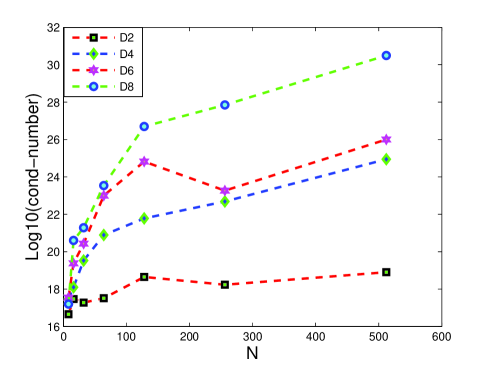
The main reason is the rapid worsening (increasing) of the condition number of the discretization matrices as both the order of differentiation and the spectral parameter (number of terms in the spectral series) get larger. For the Chebyshev differentiation matrices, the fact is illustrated in the Figure 1.
3 The Viola’s eigenvalue problem
As we do not have theoretical estimations for the spectrum of our hydrodynamic stability problem we will use the following eigenvalue problem as a benchmark one. More than that we try to make more explicit the reason we prefer to transform high order eigenvalue problems in systems of differential equations containing only second order derivatives, i.e., ”” strategy.
The Viola eigenvalue problem reads (see Straughan [29] P. 218 and the works quoted there)
| (12) |
where the parameter satisfies The problem becomes singular as
With a change of variable analogous to (7), i.e., the problem (12) reduces to an eigenvalue problem for the pair containing only Dirichlet boundary conditions, namely
As we make use of Chebyshev polynomials, the linear transformation of independent variables shifts our problem on the close interval To go further with our method we solve this eigenvalue problem by the Chebyshev collocation method. This method transforms the problem into the following generalized algebraic eigenvalue problem
| (13) |
where the matrices and are
| (14) |
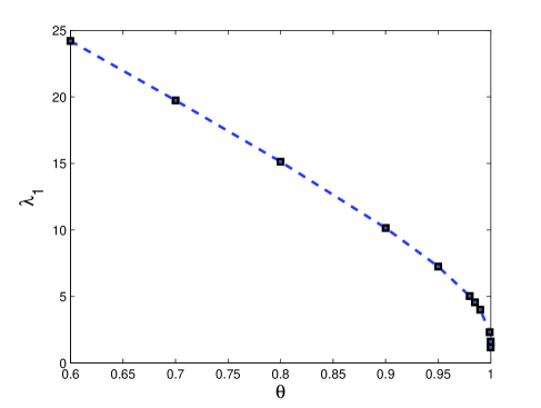
and the submatrices and stand respectively for the second order differentiation matrix on the Chebyshev nodes of the second kind the unitary matrix of order and the matrix with all zero entries of order It is important to underline that in the differentiation matrix the boundary conditions are enforced, thus the rows and columns corresponding to the first node and the last node are deleted. The vector contains the values of the approximations of and in the nodes of , i.e., . All the differentiation matrices we have used (chebdif,cheb2bc) come from the work of Weideman and Reddy [32]. The problem (13) was solved using the MATLAB code eig. Our results confirm up to some point those of Straughan [29]. Apart from those we conjecture that the first eigenvalue approaches as ! It is sustained by the numerical results reported in Figure 2. They were obtained when and corresponding to we got More than that, for and the same we obtained We have to observe that all the computations involved by the collocation method were performed in full precision (64 bit arithmetic).
An inconvenience of our approach consists in the fact that corresponding to all zero rows in the matrix the eigenvalues equal infinity (the rank of matrix equals . The MATLAB code eig, which implements the qz algorithm and gives access to intermediate results in the computation of generalized eigenvalues, explains this phenomenon. In fact the generalized eigenvalues for those zero rows are zero.
As a further check on accuracy, we computed two types of sensitivities defined as
| (15) |
for the eigenvalue where and are the right and left eigenvectors of (13) respectively. They were introduced by Stewart and Sun in [28] and used in an analogous problem by Dongarra et al. in [5]. Corresponding to Chebyshev collocation method applied to problem (13) with we summarize the situation in the Table 1.
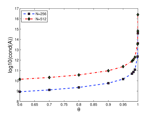
It is fairly clear from this table that both measures of sensitivities increase drastically with the decreasing of parameter In other words, the more singular is the differential problem the more sensitive are the eigenvalues. Since the quantity is a measure of the number of digits one lose in accuracy this table provide useful information on the accuracy of the actual computations. A similar conclusion provides the Figure 3. As the curves versus for and respectively, are quite parallel and horizontal for they sharply increase for
An attempt was made to solve the problem (12) as a sixth order one. In order to fulfill the boundary conditions we use this time the more complicated weighted functions
and in order to obtain the corresponding differentiation matrices we make use of the code poldif from the same paper of Weideman and Reddy [32]. In this situation the right hand side matrix of the generalized eigenvalue problem is a diagonal one and consequently it is easy invertible. This way we are in the situation to solve an usual eigenvalue problem. For values of around the MATLAB code qz as well as the MATLAB code invshift (see Quarteroni and Saleri [24] P. 175) which evaluates the eigenvalue of minimum modulus of a matrix by the inverse power method, provide positive values for However, they are far larger than those obtained above. For beyond the situation is even worse. The eigenvalue of minimum modulus becomes negative and also complex eigenvalues appear in the spectrum. This means numerical instability.
4 Spectral methods for hydrodynamic stability problem (4)-(6)
Actually we look for the smallest eigenvalue (the Rayleigh number) in the problem (8)-(9) defining the neutral manifold.
In order to accomplish that, we reduce the problem to generalized algebraic eigenvalue first by a weighted residual (Galerkin) type method. To this end we formulate the eigenvalue problem in an operatorial framework by introducing the vectorial unknown as , the operator and the functional space where
and
and stand for the identity and null operator. The space is a subspace of the Sobolev space Endowed with the inner product defined as usual by with the weight it is a Hilbert space. When we suppress this index from the definition of the scalar product.
It is clear that is invertible and does not have this property.
As in the case of Viola’s problem we first translate the problem on the interval
Consequently, our problem reads: find and such that
| (16) |
Various numerical methods can be used in order to solve the problem (16). In the monographs [2], [3], [19] or [30] to quote but a few, details on the spectral methods are provided including the approximation results in the weighted Sobolev spaces In our recent monograph [12] we tried to collect some classical and at the same time difficult eigenvalue problems and compare the results obtained by spectral methods with their exact solutions or at least other numerical results (see [23] for such a collection).
Let us consider the following two finite dimensional spaces , , both subspaces of , made up by functions which satisfy the Dirichlet boundary conditions at In our case an approximation of the solution has the form , with the index related to the discretization process. As usual, , , are defined as truncated series of orthogonal functions (trial functions)
| (17) |
In (17) the coefficients , , , are unknown and the sets , , are the sets of trial functions. This imply . The spectral approximation is obtained by imposing the vanishing of the projection of the residual on the finite dimensional space , subspace of , so a general weighted residual formulation for the problem (16) reads: find and such that
| (18) |
Whenever we perform an integration by parts of in the above formulation, in order to lower the order of differentiation, the formulation is called week and the method becomes a Galerkin-Petrov one. When the space of trial functions and that of test functions are identical we come up with the well known Galerkin method.
In [9] the analytical study of the eigenvalue problem (8)-(9) was performed by using complete sets of orthogonal functions directly on , i.e. shifted Chebyshev and Legendre polynomials.
For the particular varying gravity field we solve the problem (18) using several basis in the test and trial spaces.
i) Weighted residuals (Galerkin) methods (WRG). We considered two family of functions as basis of the finite dimensional spaces , . They have the form with the Shen basis (SB1) [27] defined by
| (19) |
and , which is another Shen basis (SB2)[27], having the form
| (20) |
Then, in each case, the unknowns , , are approximated respectively by
Let us introduce the vector of the unknown coefficients , , by
With this notation the equation (18) becomes
| (21) |
where the matrix is defined by
which means a homogeneous linear algebraic system of equations and unknowns.
The corresponding secular equation has the form
| (22) |
with
For the Galerkin method the secular equation becomes
ii) Weighted residuals (Petrov-Galerkin) methods (WRPG). We considered two variants. At first, in the method (WRPG1), the set of trial functions is of the form with the Heinrich’s basis ([14]) defined as
| (23) |
and the set of test functions is defined as before. For the second variant (WRPG2) we choose the same set of trial functions as for (WRPG1) and as a set of test functions we choose .
The secular equation is obtained the same way as in the WRG method.
iii) Collocation methods. The Chebyshev collocation method, (CC) for short, reduces the eigenvalue problem (8)-(9) to an algebraic problem of the form (13) where the matrices and are now
with the same significance for matrices and but is the diagonal matrix The numerical results obtained for various values of and with are reported in the last column of the Table 3. They were obtained using the same MATLAB code eig.
With respect to the sensitivity defined by (15) we remark that this problem is less sensitive than the singularly perturbed Viola’s problem. For the first indicator we obtained which increases to and slightly oscillates around . It is important that they remains practically independent of
5 Numerical results
Numerical evaluations of the Rayleigh number for the particular case in which the gravity variation is are given. For comparison, we present in Table 2, our previous evaluations of the Rayleigh number from [6], [9]. These evaluations are obtained by spectral methods based on shifted Chebyshev polynomials (SCP), shifted Legendre polynomials (SLP) and trigonometric series (TS). The numerical results obtained here by the weighted residual Galerkin methods (WRG)(presented in Table 3) (for the first Shen basis (WRG(SB1)) and for the second Shen basis (WRG(SB2)) are similar to the ones in Table 2 and underline the same physical conclusion that a linearly decreasing variable gravity field enlarges the domain of stability. The evaluations obtained by the Chebyshev collocation method (CC) are presented in the last column of the same table.
Then numerical evaluations of , obtained for the two variants of the weighted residual Petrov-Galerkin method (WRPG1 and WRPG2), are displayed in the Table 4. These numerical results are similar. However, the use of the (WRPG) method simplifies the numerical evaluations and reduces the time of computation due to the fact that a larger number of scalar products in the secular equation vanish.
All in all, comparing the Tables 2, 3 and 4 it is fairly clear that the Chebyshev collocation method and the Galerkin method based on trigonometric polynomials provide the closest results.
The numerical scheme for the generation of the spectrum in the case of weighted residual methods based on trigonometric and polynomial expansions is a Maple code which implements the LU decomposition. In Table 5 the Rayleigh number for the classical case [4], i.e. , , obtained by (WRG) with the first Shen basis are shown. The results are presented, for various spectral orders, in comparison with the necessary time for each evaluation. It is noticed that a larger spectral order is time consuming without having a distinctive improvement of the numerical results.
We can conclude that for a relatively small , i.e., fairly accurate numerical results are obtained using these methods. However, for larger the computational time highly increases, without leading to a significant improvement of the numerical values (less than ).
A better situation is observed with respect to the collocation method. The spectral order used is much more large than that used in the weighted residual methods, i.e., is of order with . In spite of this, our numerical experiments showed that the collocation methods are much more rapid (the CPU time increases moderately with ) and more flexible with respect to the implementation process. However, both classes of methods provide reliable approximations for the lower part of the spectra. More than that, they do not require assumptions on the scale resolution, i.e., that is small, as it is the case with the methods considered by Melenk, Kirkner and Schwab in [20].
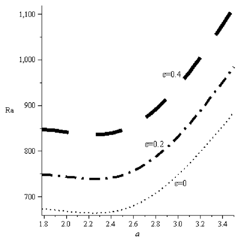
In Fig. 4 graphical representations of the neutral curves
for different values of the scale parameter are given, pointing out its
influence on the stability domain.
6 Conclusions
In this paper a numerical study of a linear hydrodynamic stability problem of a convective flow in the presence of a varying gravity field is carried out. The sixth order eigenvalue problem with Dirichlet and hinged boundary conditions is cast into a second order eigenvalue problem supplied only with Dirichlet boundary conditions. It is solved by some weighted residual methods (Galerkin type) methods as well as by a collocation method. The algorithm is fairly general and its Chebyshev collocation implementation very fast and flexible. Formally this implementation produces some spurious eigenvalues but this fact is explicable and expected. However, the lower part of the spectrum, which is highly important, is accurately approximated. More than that, no scale resolution restrictions are required.
The Chebyshev collocation version of our method was validated in solving the Viola eigenvalue problem. It is a singular eigenvalue problem with high sensitive eigenvalues. About this problem we conjecture that the first eigenvalue as
Acknowledgements
The research of the second author was supported in part by the CEEX Grant 2-CEx06-11-96/19.09.2006. The authors are fairly grateful to the two anonymus referees for their careful reading of the paper and trenchant suggestions for improvement.
References
- [1] Blyth, M. G., Pozrikidis, C., Effect of surfactant on the stability of film flow down an inclined plane, J. Fluid Mech. 521 (2004) 241-250.
- [2] Boyd, J. P., Chebyshev and Fourier spectral methods, 2nd. Ed., Dover, New York, 2000.
- [3] Canuto, C., Hussaini, M.Y., Quarteroni, A., Zang, T.A., Spectral Methods in Fluid Dynamics, Springer Verlag, 1987.
- [4] Chandrasekhar, S., Hydrodynamic and hydromagnetic stability, Oxford Univ. Press, 1961.
- [5] Dongarra, J. J., Straughan, B., Walker, D. W., Chebyshev tau-QZ algorithm methods for calculating spectra of hydrodynamic stability problems, Appl. Numer. Math. 22 (1996) 399-434.
- [6] Dragomirescu, I., Approximate neutral surface of a convection problem for variable gravity field, Rend. Sem. Mat. Univ. Pol. Torino 64 (2006) 331-342.
- [7] Dragomirescu, I., Georgescu, A., Linear stability bounds in a convection problem for variable gravity field, ASM Bull. Matematica 52 (2006) 51-56.
- [8] Dragomirescu, I., A SLP-based method for a convection problem for a variable gravity field, in Proc. of Aplimat 2007, Bratislava, pp. 149-154.
- [9] Dragomirescu, I., Shifted polynomials in a convection problem, Appl. Math. & Inf. Sc. J 2 2 (2008) 163-172.
- [10] Drazin, P.G., Reid, W. H., Hydrodynamic stability, Cambridge University Press, London, 1981.
- [11] Gheorghiu, C. I., Pop, I. S., A Modified Chebyshev-tau Method for a Hydrodynamic Stability Problem, in Proc. ICAOR ’97, vol. II, Transilvania Press, Cluj-Napoca, 1997, pp. 119-126.
- [12] Gheorghiu, C. I., Spectral methods for differential problems, Casa Cartii de Stiinta Publishing House, Cluj-Napoca, 2007.
- [13] Greenberg, L., Marleta, M., Numerical Solution of Non-Self-Adjoint Sturm-Liouville Problems and Related Systems, SIAM J. Numer. Anal. 38 (2001) 1800-1845.
- [14] Heinrichs, W., Improved Condition Number for Spectral Methods, Math. Comput. 53 (1998) 103-119.
- [15] Herron, I., On the principle of exchange of stabilities in Rayleigh-Bénard convection, SIAM J. Appl. Math. 61 (2000) 1362-1368.
- [16] Herron, I., Onset of convection in a porous medium with internal heat source and variable gravity, Int. J Eng. Sci. 39 (2001) 201-208.
- [17] Hill, A.A., Straughan, B., A Legendre spectral element method for eigenvalues in hydromagnetic stability, J Comput. Appl. Math. 193 (2003) 363-381.
- [18] Huang, W., Sloan, D. M., The pseudospectral methods for third-order differential equations, SIAM J. Numer. Anal. 29 (1992) 1626-1647.
- [19] Mason, J.C., Handscomb, D.C., Chebyshev polynomials, Chapman & Hall, 2003.
- [20] Melenk, J. M., Kirkner, N. P., Schwab, V., Spectral Galerkin Discretization for Hydrodynamic Stability Problems, Computing 65 (2000) 97-118.
- [21] Orszag, S., Accurate solutions of Orr-Sommerfeld stability equation, J. Fluid Mech. 50 (1971) 689-703.
- [22] Prakash, K., Raj, H., Effect of variable gravitational field on thermal instability of a rotating fluid layer with magnetic field in porous medium, Czech. J. of Physics 47 (1997) 793-800.
- [23] Pruess, S., Fulton, C.T., Mathematical Software for Sturm-Liouville Problems, ACM Trans. Softw. 19 (1998) 360-376.
- [24] Quarteroni, A., Saleri, F., Scientific Computing with MATLAB and Octave, Second Edition, Springer Verlag, 2006
- [25] Reddy, S. C., Schmid, P. J., Henningson, D., Pseudospectra of Orr-Sommerfeld operator, SIAM J. Appl. Math. 53 (1993) 15-47.
- [26] Shen, J., Efficient spectral-Galerkin method I, Direct solvers of second and fourth order equations by using Legendre polynomials, SIAM J. on Sci. Comput. 15 (1994) 1489-1505.
- [27] Shen, J., Efficient spectral-Galerkin method II, Direct solvers of second and fourth order equations by using Chebyshev polynomials, SIAM J. on Sci. Comput. 16 (1995) 74-87.
- [28] Stewart, G.W., Sun, J.-G., Matrix Perturbation Theory, Academic Press, New York, 1990.
- [29] Straughan, B., The energy method, stability, and nonlinear convection, Springer, Berlin, 2003.
- [30] Trefethen, L.N., Spectral Methods in MATLAB, SIAM Philadelphia, PA, 2000.
- [31] Vekilov, P.G., Protein Crystal Growth – Microgravity Aspects, Advances in Space Research 24 (1999) 1231-1240.
- [32] Weideman, J. A. C., Reddy, S. C., A MATLAB Differentiation Matrix Suite, ACM Trans. on Math. Software 26 (2000) 465-519.
[1] M.G. Blyth, C. Pozrikidis, Effect of surfactant on the stability of film flow down an inclined plane, J. Fluid Mech. 521 (2004) 241–250.
[2] J.P. Boyd, Chebyshev and Fourier Spectral Methods, second ed., Dover, New York, 2000.
[3] C. Canuto, M.Y. Hussaini, A. Quarteroni, T.A. Zang, Spectral Methods in Fluid Dynamics, Springer-Verlag, 1987.
[4] S. Chandrasekhar, Hydrodynamic and Hydromagnetic Stability, Oxford Univ. Press, 1961.
[5] J.J. Dongarra, B. Straughan, D.W. Walker, Chebyshev tau-QZ algorithm methods for calculating spectra of hydrodynamic stability problems, Appl. Numer. Math. 22 (1996) 399–434.
[6] I. Dragomirescu, Approximate neutral surface of a convection problem for variable gravity field, Rend. Sem. Mat. Univ. Politec Torino 64 (2006) 331–342.
[7] I. Dragomirescu, A. Georgescu, Linear stability bounds in a convection problem for variable gravity field, Bul. Acad. Stiinte Repub. Mold. Mat. 52 (2006) 51–66.
[8] I. Dragomirescu, A SLP-based method for a convection problem for a variable gravity field, in: Proc. of Aplimat 2007, Bratislava, pp. 149–154.
[9] I. Dragomirescu, Shifted polynomials in a convection problem, arXiv:0709.2240v1 [math-ph], 2007.
[10] P.G. Drazin, W.H. Reid, Hydrodynamic Stability, Cambridge University Press, London, 1981.
[11] C.I. Gheorghiu, I.S. Pop, A modified Chebyshev-tau method for a hydrodynamic stability problem, in: Proc. ICAOR ’97, vol. II, Transylvania Press, Cluj-Napoca, 1997, pp. 119–126.
[12] C.I. Gheorghiu, Spectral Methods for Differential Problems, Casa Cartii de Stiinta Publishing House, Cluj-Napoca, 2007.
[13] L. Greenberg, M. Marleta, Numerical solution of non-self-adjoint Sturm–Liouville problems and related systems, SIAM J. Numer. Anal. 38 (2001) 1800–1845.
[14] W. Heinrichs, Improved condition number for spectral methods, Math. Comput. 53 (1998) 103–119.
[15] I. Herron, On the principle of exchange of stabilities in Rayleigh–Bénard convection, SIAM J. Appl. Math. 61 (2000) 1362–1368.
[16] A.A. Hill, B. Straughan, A Legendre spectral element method for eigenvalues in hydromagnetic stability, J. Comput. Appl. Math. 193 (2003) 363–381.
[17] W. Huang, D.M. Sloan, The pseudospectral methods for third-order differential equations, SIAM J. Numer. Anal. 29 (1992) 1626–1647.
[18] J.C. Mason, D.C. Handscomb, Chebyshev Polynomials, Chapman & Hall, 2003.
[19] J.M. Melenk, N.P. Kirkner, V. Schwab, Spectral Galerkin discretization for hydrodynamic stability problems, Computing 65 (2000) 97–118.
[20] S. Orszag, Accurate solutions of Orr–Sommerfeld stability equation, J. Fluid Mech. 50 (1971) 689–703.
[21] K. Prakash, H. Raj, Effect of variable gravitational field on thermal instability of a rotating fluid layer with magnetic field in porous medium, Czech. J. Phys. 47 (1997) 793–800.
[22] S. Pruess, C.T. Fulton, Mathematical software for Sturm–Liouville problems, ACM Trans. Softw. 19 (1998) 360–376.
[23] A. Quarteroni, F. Saleri, Scientific Computing with MATLAB and Octave, second ed., Springer-Verlag, 2006.
[24] S.C. Reddy, P.J. Schmid, D. Henningson, Pseudospectra of Orr–Sommerfeld operator, SIAM J. Appl. Math. 53 (1993) 15–47.
[25] J. Shen, Efficient spectral-Galerkin method II, Direct solvers of second and fourth order equations by using Chebyshev polynomials, SIAM J. Sci. Comput. 16 (1995) 74–87.
[26] G.W. Stewart, J.-G. Sun, Matrix Perturbation Theory, Academic Press, New York, 1990.
[27] B. Straughan, The Energy Method, Stability, and Nonlinear Convection, Springer, Berlin, 2003.
[28] L.N. Trefethen, Spectral Methods in MATLAB, SIAM, Philadelphia, PA, 2000.
[29] P.G. Vekilov, Protein crystal growth—microgravity aspects, Advances in Space Research 24 (1999) 1231–1240.
[30] J.A.C. Weideman, S.C. Reddy, A MATLAB differentiation matrix suite, ACM Trans. on Math. Software 26 (2000) 465–519.