Spherical interpolation of scattered data using least squares thin-plate spline and inverse multiquadric functions

3 months ago

(original), approximation of multivariate functions, Approximation Theory, interpolation, ISI/JCR, paper, Shepard, splines

Abstract

We construct some smooth functions defined over a sphere that interpolate large sets of scattered data, using some modified Shepard methods, the least squares thin-plate spline and the inverse multiquadric functions. We illustrate the benefits of our methods in numerical examples for some test functions and some real data applications.

Authors

Teodora Cătinaş
Faculty of Mathematics and Computer Science, Babeş-Bolyai University, Cluj-Napoca, Romania

Andra Malina
Faculty of Mathematics and Computer Science, Babeş-Bolyai University, Cluj-Napoca, Romania
Tiberiu Popoviciu Institute of Numerical Analysis, Romanian Academy, Cluj-Napoca, Romania

Keywords

Interpolation of scattered data; Sphere; Shepard operator; Least squares approximation; Thin plate spline; Inverse multiquadric; Spiral points; Error estimations

Paper coordinates

T. Catinas, A. Malina, Spherical interpolation of scattered data using least squares thin-plate spline and inverse multiquadratic functions, Numerical Algorithms, 2024, https://doi.org/10.1007/s11075-024-01755-6

PDF

About this paper

Journal

Numerical Algorithms

Publisher Name

Springer Link

DOI

https://doi.org/10.1007/s11075-024-01755-6

Print ISSN

1572-9265

Online ISSN

1017-1398

google scholar link

Paper (preprint) in HTML form

Spherical interpolation of scattered data using least squares thin-plate spline and inverse multiquadric functions

Spherical interpolation of scattered data using
least squares thin-plate spline and
inverse multiquadric functions

Teodora Cătinaş¹ and Andra Malina^1,2

Abstract.

Keywords: Interpolation of scattered data, sphere, Shepard operator, least squares approximation, thin plate spline, inverse multiquadric, spiral points, error estimations.

MSC 2020 Subject Classification: 41A05, 41A25, 41A80, 65D05, 65D15, 65D12, 33C55.

¹Babeş-Bolyai University, Faculty of Mathematics and Computer Science, Str. M. Kogălniceanu Nr. 1, RO-400084 Cluj-Napoca, Romania, e-mails: teodora.catinas@ubbcluj.ro (corresponding author), andra.malina@ubbcluj.ro.

²Tiberiu Popoviciu Institute of Numerical Analysis, Romanian Academy, Cluj-Napoca, Romania.

1. Preliminaries

We consider here the problem of interpolating large scattered data sets lying on a sphere by using a Shepard type method and some radial basis functions. This interpolation problem is important as it appears in solving some problems related to some physical phenomenons, such as temperature, rainfall, pressure, ozone or gravitational forces, measured at various points on the surface of the Earth; they could also be applied in modelling closed surfaces in CAGD, see, e.g., [7]. As it is mentioned in [9] and [25], these type of data fitting problems, where the underlying domain is the sphere, arises in many areas, including, e.g., geophysics and meteorology, as, in general, the sphere is taken as a model of the Earth. Many authors have investigated the approximation of functions on the sphere by means of polynomials or radial basis functions (see, e.g, [1], [2], [7]-[12], [17], [19], [25]), the main motivation being the need to approximate geophysical quantities.

The Shepard method, introduced in [24], is one of the best suited methods for approximating large sets of data. It has the advantages of a small storage requirement and an easy generalization to additional independent variables, but it suffers from no good reproduction quality, low accuracy and a high computational cost relative to some alternative methods [22], these being the reasons for finding new methods that improve it (see, e.g., [3]-[6], [13], [20], [27]). The radial basis functions are suitable tools for scattered data, and for data that varies rapidly over short distances.

Our purpose in this paper is to introduce some combined Shepard methods using the least squares thin-plate spline and the inverse multiquadric functions, so our method involves also least squares approximation method, not just radial basis functions as, for example, in [9], [12] and [25].

Combined polynomial and radial basis function approximations have often been studied in the context of radial basis functions constructed from conditionally positive definite kernels, in which case a polynomial part is needed to make the theory work. Here, we restrict our attention to the case of (conditionally) strictly positive definite kernels, including a polynomial component, motivated by the fact that approximations of this kind offer real advantages.

The numerical tests on different types of data prove the efficiency of the method. Moreover, a physical phenomenon is investigated, namely temperature prediction on the Earth’s surface, and the results show that this method is a powerful instrument for solving various problems that model real life phenomena.

2. Combined spherical Shepard method

Following the idea and some notations from [7], we introduce several modifications of the spherical Shepard method using spherical radial basis functions.

Let $S\$ be the unit sphere in $\mathbb{R}^{3}$ centered at the origin. Let us consider the set of distinct nodes $\mathbf{x}_{i}=(x_{i},y_{i},z_{i}),i=1,...,n$ , lying on $S$ and the corresponding function values $f_{i},i=1,...,n$ , with $f:S\to\mathbb{R}$ . For $\mathbf{x}=(x,y,z)\in S$ the modified spherical Shepard operator is defined as (see, e.g., [7])

(2.1)

S(\mathbf{x})=\frac{{\textstyle\sum\limits_{j=1}^{n}}w_{j}(\mathbf{x})f_{j}}{{% \textstyle\sum\limits_{k=1}^{n}}w_{k}(\mathbf{x})},

with

(2.2)

w_{j}\left(\mathbf{x}\right)=\left[\tfrac{(R^{w}_{j}-g(\mathbf{x},\mathbf{x}_{% j}))_{+}}{R^{w}_{j}g(\mathbf{x},\mathbf{x}_{j})}\right]^{2},

and $R_{j}^{w}$ is a radius of influence about the node $j$ and the geodesic distance $g$ between $\mathbf{x}$ and $\mathbf{x}_{j}$ defined as

(2.3)

g(\mathbf{x},\mathbf{x}_{j})=\arccos(\mathbf{x}\cdot\mathbf{x}_{j}),

where $u_{+}=\max\{0,u\}$ and ${}^{\prime\prime}\cdot^{\prime\prime}$ denotes the Euclidean inner product of the two vectors.

For a set of scattered data $X=\{\mathbf{x}_{1},\mathbf{x}_{2},...,\mathbf{x}_{n}\}$ the mesh norm $h_{X}$ is defined by $h_{X}=\sup\limits_{x\in S}g(x,X),$ where $g$ denotes the geodesic distance.

If we denote by (see, e.g., [7])

\overline{w}_{j}(\mathbf{x})=\frac{w_{j}(\mathbf{x})}{{\textstyle\sum\limits_{% k=1}^{n}}w_{k}(\mathbf{x})},

then we have the following properties of the weights:

1.

the cardinality property: $\overline{w}_{j}(\mathbf{x}_{i})=\delta_{ij}$ ;
2.

the partition of unity property: $\sum\limits_{j=1}^{n}\overline{w}_{j}(\mathbf{x})=1$ .

Definition 2.1.

(see, e.g., [19]) Let $\psi:[0,\pi]\to\mathbb{R}$ be a continuous function. We say that $\psi$ is strictly positive definite on $S$ ( $\psi\in$ SPD) if, for any set of $n$ distinct points $\mathbf{x}_{i},\;i=1,...,n,$ lying on $S$ , the quadratic form

(2.4)

\sum\limits_{j=1}^{n}\sum\limits_{k=1}^{n}a_{j}a_{k}\psi(g(\mathbf{x}_{j},% \mathbf{x}_{k}))

is positive on $\mathbb{R}^{n}\setminus\{\mathbf{0}\}$ .

We recall some notions from [19]. A polynomial $p:\mathbb{R}^{3}\to\mathbb{R}$ of degree $d,\;d\geq 0$ is homogeneous of degree $d$ if $p(t\mathbf{x})=t^{d}p(\mathbf{x})$ , for any $\mathbf{x}\in\mathbb{R}^{3}$ and $t>0$ . The polynomial $p$ is harmonic if $\Delta p(\mathbf{x})=0$ , for any $\mathbf{x}\in\mathbb{R}^{3}$ , where $\Delta$ is the Laplace operator, i.e.,

\Delta p=\frac{\partial^{2}p}{\partial x^{2}}+\frac{\partial^{2}p}{\partial y^% {2}}+\frac{\partial^{2}p}{\partial z^{2}}.

So, if $\mathcal{P}_{d}$ is the set of polynomials of degree $d$ in $\mathbb{R}^{3}$ that are harmonic and homogeneous of order $d$ , we can define the set

\mathcal{H}_{d}^{*}(S)=\{p|_{S}:\;p\in\mathcal{P}_{d}\}

of spherical harmonics of exact order $d$ . The dimension of $\mathcal{H}_{d}^{*}(S)$ is

\dim\mathcal{H}_{d}^{*}(S)=2d+1.

Denoting the space of spherical harmonics of maximum order $d$ by $\mathcal{H}_{d}(S)$ , we have

\mathcal{H}_{d}(S)=\oplus_{j=0}^{d}\mathcal{H}_{j}^{*}(S).

It follows that the dimension of $\mathcal{H}_{d}(S)$ is

\dim{H}_{d}(S)=(d+1)^{2}.

Definition 2.2.

(see, e.g., [19]) Let $\psi:[0,\pi]\to\mathbb{R}$ be a continuous function and $m$ a positive integer. We say that $\psi$ is conditionally strictly positive definite on $S$ of order $m$ ( $\psi\in$ CSPD( $m$ )) if, for any set of $n$ distinct points $\mathbf{x}_{i},\;i=1,...,n,$ lying on $S$ , the quadratic form (2.4) is positive on

W_{m-1}=\Big{\{}\mathbf{a}\in\mathbb{R}^{n}\setminus\{\mathbf{0}\}:\sum\limits% _{i=1}^{n}a_{i}y(\mathbf{x}_{i})=0\mbox{ for all }y\in\mathcal{H}_{m-1}(S)\Big% {\}}.

Definition 2.3.

(see, e.g., [7]) For a set of distinct nodes $\mathbf{x}_{i}=(x_{i},y_{i},z_{i}),i=1,...,n$ , lying on $S$ and the corresponding function values $f_{i},i=1,...,n$ , with $f:S\to\mathbb{R}$ , the zonal basis function interpolant $s^{(1)}:S\to\mathbb{R}$ is defined as

(2.5)

s^{(1)}(\mathbf{x})=\sum\limits_{j=1}^{n}a_{j}\psi(g(\mathbf{x},\mathbf{x}_{j}% )),

with the coefficients $a_{j},\;j=1,...,n$ , obtained from the interpolation relations

s^{(1)}(\mathbf{x}_{i})=f_{i},\;i=1,...,n,

where $g(\mathbf{x},\mathbf{x}_{j})$ is the geodesic distance between $\mathbf{x}$ and $\mathbf{x}_{j}$ and $\psi:[0,\pi]\to\mathbb{R}$ is a zonal basis function, i.e., the sphere analogue of the Euclidean radial basis function.

Definition 2.4.

(see, e.g., [8]) For a set of distinct nodes $\mathbf{x}_{i}=(x_{i},y_{i},z_{i}),i=1,...,n$ , lying on $S$ and the corresponding function values $f_{i},i=1,...,n$ , with $f:S\to\mathbb{R}$ , the augmented zonal basis function interpolant $s^{(2)}:S\to\mathbb{R}$ is defined as

(2.6)

s^{(2)}(\mathbf{x})=\sum\limits_{j=1}^{n}a_{j}\psi(g(\mathbf{x},\mathbf{x}_{j}% ))+\sum_{k=1}^{D}A_{k}y_{k}(\mathbf{x}),

with $D=\dim\mathcal{H}_{d}(S)$ , $\{y_{1},...,y_{D}\}$ is a basis for $\mathcal{H}_{d}(S)$ and the coefficients $a_{j},\;j=1,...,n$ , and $A_{k},k=1,...,D$ , obtained from the interpolation conditions

s^{(2)}(\mathbf{x}_{i})=f_{i},\;i=1,...,n,

and by the constraints

\sum\limits_{i=1}^{n}a_{i}y_{k}(\mathbf{x}_{i})=0,\;k=1,...,D.

Definition 2.5.

(see, e.g., [7]) Considering for each node $\mathbf{x}_{j},\;j=1,...,n$ , a set $I_{j}$ that contains the indices of $n_{Z}$ closest neighbours of $\mathbf{x}_{j}$ , we define a local zonal basis function interpolant $s_{j}^{(1)}:S\to\mathbb{R}$ as

(2.7)

s_{j}^{(1)}(\mathbf{x})=\sum\limits_{i\in I_{j}}a_{i}^{j}\psi(g(\mathbf{x},% \mathbf{x}_{j})),

with the coefficients $a_{i}^{j},\;i\in I_{j},\;j=1,...,n$ , obtained from the interpolation relations

s_{j}^{(1)}(\mathbf{x}_{i})=f_{i},\;i\in I_{j},\;j=1,...,n.

Definition 2.6.

(see, e.g., [8]) Considering for each node $\mathbf{x}_{j},\;j=1,...,n$ , a set $I_{j}$ that contains the indices of $n_{Z}$ closest neighbours of $\mathbf{x}_{j}$ , we introduce here the augmented local zonal basis function interpolant $s_{j}^{(2)}:S\to\mathbb{R}$ as

(2.8)

s_{j}^{(2)}(\mathbf{x})=\sum\limits_{i\in I_{j}}a_{i}^{j}\psi(g(\mathbf{x},% \mathbf{x}_{j}))+\sum_{k=1}^{D}A^{j}_{k}y_{k}(\mathbf{x}),

with $D=\dim\mathcal{H}_{d}(S),\;D\leq n_{Z}$ , $\{y_{1},...,y_{D}\}$ basis for $\mathcal{H}_{d}(S)$ and the coefficients $a_{i}^{j},\;i\in I_{j},\;j=1,...,n$ , and $A^{j}_{k},k=1,...,D$ , obtained from the interpolation conditions

s_{j}^{(2)}(\mathbf{x}_{i})=f_{i},\;i\in I_{j},\;j=1,...,n,

and the constraints

\sum\limits_{i\in I_{j}}a_{i}^{j}y_{k}(\mathbf{x}_{i})=0,\;j=1,...,n,\;k=1,...% ,D.

Now we introduce the new local Shepard interpolants,

(2.9)

S_{1}(\mathbf{x})=\frac{{\textstyle\sum\limits_{j=1}^{n}}w_{j}(\mathbf{x})Z_{j% }^{(1)}(\mathbf{x})}{{\textstyle\sum\limits_{k=1}^{n}}w_{k}(\mathbf{x})},

with the local zonal basis function given by

Z_{j}^{(1)}(\mathbf{x})=\sum\limits_{i\in I_{j}}a_{i}^{j}\psi_{1}(g(\mathbf{x}% ,\mathbf{x}_{i}))

and

(2.10)

S_{2}(\mathbf{x})=\frac{{\textstyle\sum\limits_{j=1}^{n}}w_{j}(\mathbf{x})Z_{j% }^{(2)}(\mathbf{x})}{{\textstyle\sum\limits_{k=1}^{n}}w_{k}(\mathbf{x})},

with

Z_{j}^{(2)}(\mathbf{x})=\sum\limits_{i\in I_{j}}a_{i}^{j}\psi_{1}(g(\mathbf{x}% ,\mathbf{x}_{i}))+\sum_{k=1}^{D}A^{j}_{k}y_{k}(\mathbf{x}),

considering the thin-plate spline spherical radial basis function (see, e.g., [2])

\psi_{1}(r)=r^{2}\log r,\;r=2\sin(t/2),\;t=g(\mathbf{x},\mathbf{y})=\arccos(% \mathbf{x}\cdot\mathbf{y}).

Remark 2.7.

[19] Based on Definition 2.2, the thin-plate spline spherical radial basis function $\psi_{1}$ is conditionally strictly positive definite on $S$ of order $2$ .

Similarly, we introduce

(2.11)

S_{3}(\mathbf{x})=\frac{{\textstyle\sum\limits_{j=1}^{n}}w_{j}(\mathbf{x})Z_{j% }^{(3)}(\mathbf{x})}{{\textstyle\sum\limits_{k=1}^{n}}w_{k}(\mathbf{x})},

with the local zonal basis function given by

Z_{j}^{(3)}(\mathbf{x})=\sum\limits_{i\in I_{j}}a_{i}^{j}\psi_{2}(g(\mathbf{x}% ,\mathbf{x}_{i}))

and

(2.12)

S_{4}(\mathbf{x})=\frac{{\textstyle\sum\limits_{j=1}^{n}}w_{j}(\mathbf{x})Z_{j% }^{(4)}(\mathbf{x})}{{\textstyle\sum\limits_{k=1}^{n}}w_{k}(\mathbf{x})},

with

(2.13)

Z_{j}^{(4)}(\mathbf{x})=\sum\limits_{i\in I_{j}}a_{i}^{j}\psi_{2}(g(\mathbf{x}% ,\mathbf{x}_{i}))+\sum_{k=1}^{D}A^{j}_{k}y_{k}(\mathbf{x}),

considering the inverse multiquadric spherical radial basis function (see, e.g., [2])

\psi_{2}(r)=(r^{2}+c^{2})^{-\frac{1}{2}},\;r=2\sin(t/2),\;t=g(\mathbf{x},% \mathbf{y})=\arccos(\mathbf{x}\cdot\mathbf{y}).

Remark 2.8.

[19] Based on Definition 2.1, the inverse multiquadric spherical radial basis function $\psi_{2}$ is strictly positive definite on $S$ .

Using a result from [20], we obtain the following estimations of the errors for the local Shepard operators introduced here.

Theorem 2.9.

Consider a set of distinct nodes $\mathbf{x}_{k},k=1,...,n,$ lying on $S$ and the corresponding function values $f_{k},k=1,...,n$ , with $f:S\to\mathbb{R}$ . For each $\mathbf{x}\in S$ , we have the following approximation of the error of the Shepard operators $S_{i},\;i=1,...,4$ , given by (2.9), (2.10), (2.11) and (2.12):

E_{i}(x)=\left|f(\mathbf{x})-S_{i}(\mathbf{x})\right|\leq\sum\limits_{j=1}^{n}% \overline{w}_{j}(\mathbf{x})e_{j}(\mathbf{x}),\ \ \ i=1,2,3,4,

with $e_{j}(\mathbf{x})=\left|f(\mathbf{x})-Z_{j}^{(i)}(\mathbf{x})\right|$ being the interpolation error of the local basis functions $Z_{j}^{(i)},\;i=1,...,4,$ on the set of nodes $\mathbf{x}_{k},\;k\in I_{j}$ , $I_{j}$ containing the indices of $n_{Z}$ closest neighbours of $\mathbf{x}_{j}$ , $j=1,...,n.$ In addition, we have

\displaystyle E_{i}(\mathbf{x})

\displaystyle\leq\max_{j=1,...,n}e_{j}(\mathbf{x}),\mbox{ for }i=1,...,4,\mbox% { and }\mathbf{x}\in S.

Proof.

	$\displaystyle E_{i}(\mathbf{x})$	$\displaystyle=\left\|f(\mathbf{x})-S_{i}(\mathbf{x})\right\|=\left\|f(\mathbf{x})% \cdot 1-\sum\limits_{j=1}^{n}\overline{w}_{j}(\mathbf{x})Z_{j}^{(i)}(\mathbf{x% })\right\|$
		$\displaystyle=\left\|f(\mathbf{x})\sum\limits_{j=1}^{n}\overline{w}_{j}(\mathbf% {x})-\sum\limits_{j=1}^{n}\overline{w}_{j}(\mathbf{x})Z_{j}^{(i)}(\mathbf{x})% \right\|=\left\|\sum\limits_{j=1}^{n}\overline{w}_{j}(\mathbf{x})\left[f(x)-Z_{j% }^{(i)}(\mathbf{x})\right]\right\|$
		$\displaystyle\leq\sum\limits_{j=1}^{n}\left\|\overline{w}_{j}(\mathbf{x})\left[% f(\mathbf{x})-Z_{j}^{(i)}(\mathbf{x})\right]\right\|=\sum\limits_{j=1}^{n}% \overline{w}_{j}(\mathbf{x})\left\|f(\mathbf{x})-Z_{j}^{(i)}(\mathbf{x})\right\|$
		$\displaystyle=\sum\limits_{j=1}^{n}\overline{w}_{j}(\mathbf{x})e_{j}(\mathbf{x% }),\mbox{ for each }i=1,...,4,\mbox{ and each }\mathbf{x}\in S.$

Since,

\displaystyle E_{i}(\mathbf{x})=\left|f(\mathbf{x})-S_{i}(\mathbf{x})\right|

\displaystyle\leq\sum\limits_{j=1}^{n}\overline{w}_{j}(\mathbf{x})\left|f(% \mathbf{x})-Z_{j}^{(i)}(\mathbf{x})\right|=\sum\limits_{j=1}^{n}\overline{w}_{% j}(\mathbf{x})e_{j}(\mathbf{x}),

we get

\displaystyle E_{i}(\mathbf{x})

\displaystyle\leq\max_{j=1,...,n}e_{j}(\mathbf{x})\sum\limits_{j=1}^{n}% \overline{w}_{j}(\mathbf{x})=\max_{j=1,...,n}e_{j}(\mathbf{x}),\mbox{ for }i=1% ,...,4,\mbox{ and }\mathbf{x}\in S.

∎

Theorem 2.10.

Consider a set of distinct nodes $\mathbf{x}_{i},i=1,...,n,$ lying on $S$ and the corresponding function values $f_{i},i=1,...,n$ , with $f:S\to\mathbb{R}$ . For the Shepard operators $S_{1},\;S_{3}$ given in (2.9) and (2.11), respectively, we have $S_{i}(\mathbf{x})\in C^{1}(S)$ , $i=1,3$ .

Proof.

The proof follows directly from Theorem 1 of [7], considering $p=2$ . ∎

Theorem 2.11.

For $f\in C(S)$ , the following estimation holds:

\displaystyle|S_{i}(\mathbf{x})-f(\mathbf{x})|\leq\sum\limits_{j=1}^{n}% \overline{w}_{j}(\mathbf{x})\cdot|Z_{j}^{(i)}(\mathbf{x})-Z_{j}^{(i)}(\mathbf{% x}_{j})|+\omega(f,h_{X}),\;\mbox{for}\ i=1,...,4,

where $\omega(f,h_{X})$ = $\sup\limits_{d(\mathbf{x},\mathbf{y})\leq h_{X}}|f(\mathbf{x})-f(\mathbf{y})|$ is the modulus of continuity of $f .$

Proof.

	$\displaystyle\|S_{i}(\mathbf{x})-f(\mathbf{x})\|$	$\displaystyle=\left\|\sum\limits_{j=1}^{n}\overline{w}_{j}(\mathbf{x})\cdot Z_{% j}^{(i)}(\mathbf{x})-f(\mathbf{x})\cdot\sum\limits_{j=1}^{n}\overline{w}_{j}(% \mathbf{x})\right\|=\left\|\sum\limits_{j=1}^{n}\overline{w}_{j}(\mathbf{x})% \cdot[Z_{j}^{(i)}(\mathbf{x})-f(\mathbf{x})]\right\|$
		$\displaystyle=\left\|\sum\limits_{j=1}^{n}\overline{w}_{j}(\mathbf{x})\cdot[Z_{% j}^{(i)}(\mathbf{x})-f(\mathbf{x}_{j})+f(\mathbf{x}_{j})-f(\mathbf{x})]\right\|$
		$\displaystyle\leq\sum\limits_{j=1}^{n}\overline{w}_{j}(\mathbf{x})\cdot\|Z_{j}^% {(i)}(\mathbf{x})-f(\mathbf{x}_{j})\|+\sum\limits_{j=1}^{n}\overline{w}_{j}(% \mathbf{x})\cdot\|f(\mathbf{x}_{j})-f(\mathbf{x})\|$
		$\displaystyle\leq\sum\limits_{j=1}^{n}\overline{w}_{j}(\mathbf{x})\cdot\|Z_{j}^% {(i)}(\mathbf{x})-Z_{j}^{(i)}(\mathbf{x}_{j})\|+\omega(f,h_{X}),\ \ i=1,...,4.$

∎

3. Test results

•

Numerical results on test functions

We use the following test functions (see, e.g., [15], [16], [21], [22]) to illustrate the theoretical results:

\begin{array}[c]{ll}f_{1}(x,y,z)&=\frac{3}{4}\exp\left[-\frac{(9x-2)^{2}+(9y-2% )^{2}+(9z-2)^{2}}{4}\right]+\frac{3}{4}\exp\left[-\frac{(9x+1)^{2}}{49}-\frac{% 9y+1}{10}-\frac{9z+1}{10}\right]+\\ &+\frac{1}{2}\exp\left[-\frac{(9x-7)^{2}+(9y-3)^{2}+(9z-5)^{2}}{4}\right]-% \frac{1}{5}\exp\left[-(9x-4)^{2}-(9y-7)^{2}-(9z-5)^{2}\right],\\ f_{2}(x,y,z)&=\frac{\left[1.25+\cos(5.4y)\right]\cdot\cos(6z)}{6+6(3x-1)^{2}},% \\ f_{3}(x,y,z)&=\exp{\left[-\frac{81}{16}\cdot\left((x-0.5)^{2}+(y-0.5)^{2}+(z-0% .5)^{2}\right)\right]}/3,\\ f_{4}(x,y,z)&=\exp{\left[-\frac{81}{4}\cdot\left((x-0.5)^{2}+(y-0.5)^{2}+(z-0.% 5)^{2}\right)\right]}/3.\end{array}

We consider two cases for the choice of nodes and points on which the operators are constructed.

For the first case, we evaluate the operators on 1000 random points on the unit sphere $S$ , using sets of 500, 1000 and 2000 spiral nodes, respectively. These nodes are constructed based on a method proposed in [23]. To describe them, we use their spherical coordinates

\mathbf{x}_{j}=\left(\cos\theta_{j}\sin\varphi_{j},\sin\theta_{j}\sin\varphi_{% j},\cos\varphi_{j}\right),\;1\leq j\leq n,

with

\begin{array}[c]{ll}&\theta_{1}=\theta_{n}=0,\;\theta_{j}=\theta_{j-1}+3.6% \cdot\left[n(1-h_{j}^{2})\right]^{-1/2},\;2\leq j\leq n-1,\\ &\varphi_{j}=\arccos h_{j},\;h_{j}=-1+2(j-1)/(n-1),\;1\leq j\leq n.\end{array}

In Tables 1 and 2 we list the maximum absolute errors (MAEs) and the root mean square errors (RMSEs) for the thin-plate spline case, given in (2.9) and for the inverse multiquadric case, given in (2.11).

The shape parameter $c$ in the inverse multiquadric case, we have computed as $1/(0.815d),$ where $d=\frac{1}{n}\sum\limits_{i=1}^{n}d_{i}$ , with $d_{i}$ being the distance from the node $i$ to its closest neighbour, following the idea proposed by Hardy in [18]. We also used the method proposed in [14, Program 2], but the results are comparable.

We consider also the case of zonal basis functions combined with spherical harmonics. For $S_{2}$ and for $S_{4}$ , given in (2.10) and (2.12), we take the particular cases

Z_{j}^{(2k)}(\mathbf{x})=\sum\limits_{i\in I_{j}}a_{i}^{j}\psi_{k}(g(\mathbf{x% },\mathbf{x}_{i}))+A^{j}x+B^{j}y+C^{j}z,\;k=1,2.

Tables 3 and 4 contain the approximation errors for $S_{2}$ and $S_{4}$ .

Numerical experiments have shown that in our cases, a good value for the number of closest neighbours of a node is $n_{Z}=17$ , but its choice is not an easy task, since there are many factors that could influence the numerical results, as it is also emphasized in [10].

We also show the computational times (CPU) of the methods considered above. Comparing the approximation results, one can see that in most of the cases, the thin-plate spline function is slightly more accurate, although good results were obtained in the case of inverse multiquadric function as well. For both zonal basis functions, the addition of a spherical harmonic produces an improved accuracy in the majority of cases, the computational times being quite equivalent.

	Nr. nodes	MAE	RMSE	CPU (s)
	$500$	$3.2578e-02$	$2.2321e-05$	$117.85$
$f_{1}$	$1000$	$2.2958e-02$	$9.9540e-06$	$314.53$
	$2000$	$1.1860e-02$	$4.6365e-06$	$692.82$
	$500$	$3.1537e-02$	$2.7775e-05$	$109.41$
$f_{2}$	$1000$	$2.6771e-02$	$2.7090e-05$	$314.45$
	$2000$	$2.2190e-02$	$1.7779e-05$	$688.81$
	$500$	$7.3569e-03$	$2.8918e-06$	$115.79$
$f_{3}$	$1000$	$6.0472e-03$	$1.5925e-06$	$315.37$
	$2000$	$2.8635e-03$	$6.5172e-07$	$690.19$
	$500$	$1.7325e-03$	$1.6889e-07$	$111.82$
$f_{4}$	$1000$	$1.8758e-03$	$1.9919e-07$	$320.68$
	$2000$	$6.5981e-04$	$2.5141e-08$	$697.34$

Table 1. MAEs and RMSEs for

S_{1}

1000 random points, spiral nodes.

	Nr. nodes	$c$	MAE	RMSE	CPU (s)
	$500$	$7.79$	$1.8202e-02$	$2.1817e-05$	$116.06$
$f_{1}$	$1000$	$10.99$	$6.6561e-02$	$2.5327e-04$	$310.39$
	$2000$	$15.53$	$7.2750e-03$	$2.5776e-06$	$749.19$
	$500$	$7.79$	$2.4314e-01$	$1.0818e-03$	$119.24$
$f_{2}$	$1000$	$10.99$	$1.1027e-01$	$2.9840e-04$	$304.50$
	$2000$	$15.53$	$1.5101e-01$	$2.2838e-04$	$772.28$
	$500$	$7.79$	$1.5149e-02$	$7.5269e-06$	$120.12$
$f_{3}$	$1000$	$10.99$	$4.2372e-02$	$2.4161e-05$	$304.88$
	$2000$	$15.53$	$4.6122e-03$	$2.6350e-07$	$717.83$
	$500$	$7.79$	$2.9829e-03$	$2.6177e-07$	$118.44$
$f_{4}$	$1000$	$10.99$	$8.8486e-03$	$6.4296e-06$	$306.77$
	$2000$	$15.53$	$2.4603e-03$	$1.8618e-07$	$719.70$

Table 2. MAEs and RMSEs for

S_{3}

1000 random points, spiral nodes.

	Nr. nodes	MAE	RMSE	CPU (s)
	$500$	$1.9314e-02$	$5.5752e-06$	$122.05$
$f_{1}$	$1000$	$1.0302e-02$	$4.7440e-06$	$325.28$
	$2000$	$7.3163e-03$	$1.4137e-06$	$732.32$
	$500$	$3.0368e-02$	$3.0068e-05$	$124.85$
$f_{2}$	$1000$	$2.4868e-02$	$1.9924e-05$	$313.66$
	$2000$	$2.3958e-02$	$1.9921e-0$ 5	$726.74$
	$500$	$2.8178e-03$	$6.1637e-07$	$133.43$
$f_{3}$	$1000$	$4.1202e-03$	$8.0461e-07$	$322.11$
	$2000$	$2.0158e-03$	$1.6570e-07$	$748.56$
	$500$	$6.5754e-04$	$2.8497e-08$	$126.62$
$f_{4}$	$1000$	$2.7432e-03$	$2.2982e-07$	$317.47$
	$2000$	$4.4006e-04$	$4.3163e-09$	$740.68$

Table 3. MAEs and RMSEs for

S_{2}

1000 random points, spiral nodes.

	Nr. nodes	$c$	MAE	RMSE	CPU (s)
	$500$	$7.79$	$1.9915e-02$	$2.0435e-05$	$123.83$
$f_{1}$	$1000$	$10.99$	$4.0497e-02$	$1.3859e-05$	$316.01$
	$2000$	$15.53$	$1.4464e-02$	$4.0249e-06$	$755.33$
	$500$	$7.79$	$1.4447e-01$	$5.4102e-04$	$122.07$
$f_{2}$	$1000$	$10.99$	$1.0639e-01$	$2.7742e-04$	$318.14$
	$2000$	$15.53$	$4.4779e-01$	$1.3011e-03$	$753.00$
	$500$	$7.79$	$1.4584e-02$	$6.0139e-06$	$123.95$
$f_{3}$	$1000$	$10.99$	$7.8427e-03$	$2.9137e-06$	$333.27$
	$2000$	$15.53$	$2.3339e-03$	$3.2443e-07$	$864.04$
	$500$	$7.79$	$2.5051e-03$	$1.8973e-07$	$122.34$
$f_{4}$	$1000$	$10.99$	$9.7760e-03$	$4.8077e-06$	$326.46$
	$2000$	$15.53$	$4.9442e-03$	$7.1491e-07$	$794.43$

Table 4. MAEs and RMSEs for

S_{4}

1000 random points, spiral nodes.

In the second case, for a fair distribution of points on the sphere, as proposed in [7], we evaluate the operator on a set of 600 spiral points, using sets of 1000, 2000, 5000 Halton nodes, respectively. The Halton nodes are constructed following the method proposed in [26]. The approximation errors for the operators $S_{1}$ , $S_{3}$ are displayed in Tables 5 and 6 and the results for the particular case of operators combined with a spherical harmonic $S_{2}$ and $S_{4}$ are given in Tables 7 and 8. The same advantages as in the first case can be observed.

	Nr. nodes	MAE	RMSE
	$1000$	$7.4316e-02$	$1.7509e-05$
$f_{1}$	$2000$	$8.4188e-02$	$1.4907e-05$
	$5000$	$6.3510e-02$	$1.8522e-05$
	$1000$	$5.6039e-02$	$3.7727e-05$
$f_{2}$	$2000$	$5.0967e-02$	$3.9249e-05$
	$5000$	$4.3811e-02$	$3.6163e-05$
	$1000$	$3.5525e-02$	$9.1690e-06$
$f_{3}$	$2000$	$3.5480e-02$	$5.7143e-06$
	$5000$	$2.7195e-02$	$1.5453e-05$
	$1000$	$3.7610e-02$	$2.5880e-06$
$f_{4}$	$2000$	$4.6500e-02$	$3.5632e-06$
	$5000$	$2.4349e-02$	$2.9733e-06$

Table 5. MAEs and RMSEs for

S_{1}

600 spiral points, Halton nodes.

	Nr. nodes	$c$	MAE	RMSE
	$1000$	$16.86$	$1.9497e-01$	$1.1405e-04$
$f_{1}$	$2000$	$23.18$	$2.2827e-01$	$9.9974e-05$
	$5000$	$37.97$	$5.2255e-02$	$2.9773e-05$
	$1000$	$16.86$	$1.5185e-01$	$4.1688e-04$
$f_{2}$	$2000$	$23.18$	$7.1859e-0$ 2	$2.1580e-04$
	$5000$	$37.97$	$8.5831e-01$	$2.0718e-02$
	$1000$	$16.86$	$5.9248e-02$	$2.1246e-05$
$f_{3}$	$2000$	$23.18$	$3.4550e-02$	$8.5223e-06$
	$5000$	$37.97$	$3.3702e-02$	$3.7609e-05$
	$1000$	$16.86$	$1.2690e-01$	$4.1630e-05$
$f_{4}$	$2000$	$23.18$	$4.0462e-02$	$5.1387e-06$
	$5000$	$37.97$	$1.8915e-02$	$2.7590e-06$

Table 6. MAEs and RMSEs for

S_{3}

600 spiral points, Halton nodes.

	Nr. nodes	MAE	RMSE
	$1000$	$7.0038e-02$	$1.1291e-05$
$f_{1}$	$2000$	$7.5987e-02$	$1.0503e-05$
	$5000$	$5.9442e-02$	$8.0161e-06$
	$1000$	$4.4536e-02$	$2.5508e-05$
$f_{2}$	$2000$	$4.1134e-02$	$2.0341e-05$
	$5000$	$2.9308e-02$	$1.5827e-05$
	$1000$	$1.9029e-02$	$1.8374e-06$
$f_{3}$	$2000$	$2.0527e-02$	$1.6900e-06$
	$5000$	$1.2587e-02$	$1.0525e-06$
	$1000$	$3.4529e-02$	$2.1881e-06$
$f_{4}$	$2000$	$4.0937e-02$	$2.6213e-06$
	$5000$	$2.2381e-02$	$1.1738e-06$

Table 7. MAEs and RMSEs for

S_{2}

600 spiral points, Halton nodes.

	Nr. nodes	$c$	MAE	RMSE
	$1000$	$16.86$	$3.2990e-01$	$2.7518e-04$
$f_{1}$	$2000$	$23.18$	$2.5271e-01$	$1.1180e-04$
	$5000$	$37.97$	$9.2228e-02$	$3.7367e-05$
	$1000$	$16.86$	$1.0212e-01$	$1.6366e-04$
$f_{2}$	$2000$	$23.18$	$3.8079e-01$	$1.9570e-04$
	$5000$	$37.97$	$1.9549e-01$	$1.4872e-03$
	$1000$	$16.86$	$3.3626e-01$	$1.0873e-04$
$f_{3}$	$2000$	$23.18$	$2.1943e-02$	$2.8096e-06$
	$5000$	$37.97$	$1.8473e-02$	$7.6410e-06$
	$1000$	$16.86$	$2.7218e-01$	$1.3480e-04$
$f_{4}$	$2000$	$23.18$	$4.0405e-02$	$6.2197e-06$
	$5000$	$37.97$	$1.4059e-02$	$1.9787e-06$

Table 8. MAEs and RMSEs for

S_{4}

600 spiral points, Halton nodes.

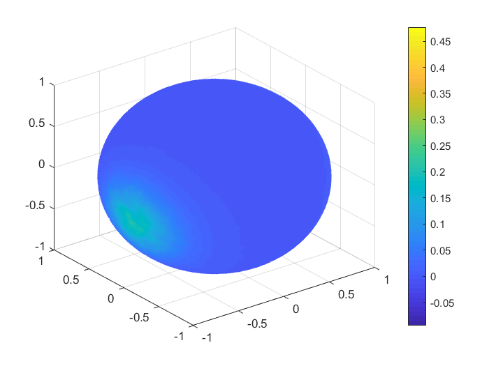
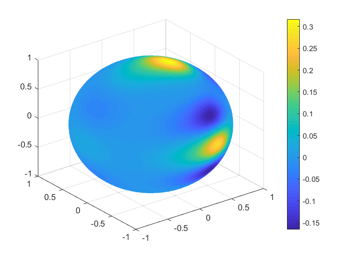
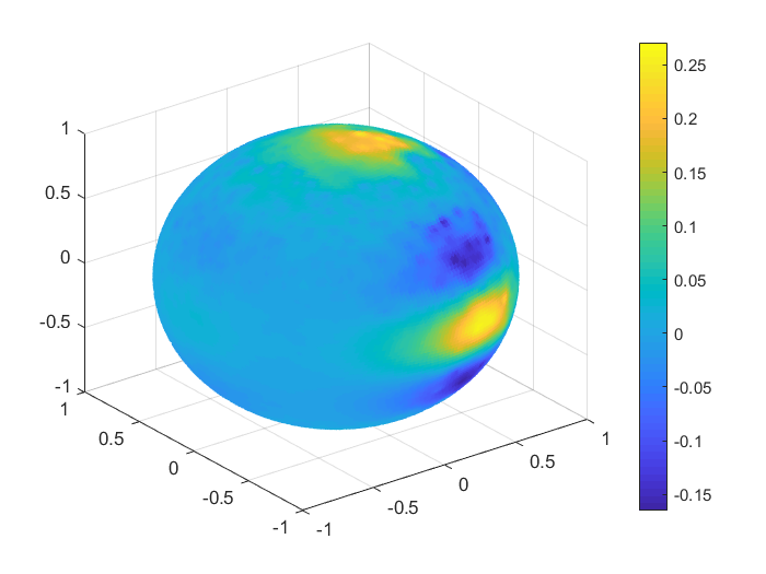
To obtain a real visualisation effect of the numerical results, in Figures 1, 2 we plot the functions values $f_{i}$ , $i=1,2$ , and the values of the corresponding Shepard interpolants $S_{1}f_{i}$ and $S_{3}f_{i}$ , $i=1,2$ , considering 1000 Halton nodes and 20000 spiral points on the unit sphere. In Table 9 we list the MAEs and the RMSEs in this case, for all the functions $f_{i},\;i=1,...,4$ .

	MAE	RMSE
$S_{1}f_{1}$	$1.2166e-01$	$2.5642e-05$
$S_{3}f_{1}$	$2.2525e-01$	$6.4609e-05$
$S_{1}f_{2}$	$5.8937e-02$	$3.8955e-05$
$S_{3}f_{2}$	$2.0732e-01$	$2.1672e-04$
$S_{1}f_{3}$	$4.3426e-02$	$1.0547e-05$
$S_{3}f_{3}$	$1.1625e-01$	$2.2429e-05$
$S_{1}f_{4}$	$3.7645e-02$	$2.0534e-06$
$S_{3}f_{4}$	$2.9282e-01$	$4.1192e-05$

Table 9. MAEs and RMSEs for the graphical representations,

20.000 spiral points, 1000 Halton nodes.

Finally, we compared our results with the ones obtained in the case of the modified spherical Shepard operator $S$ , defined in (2.1). In Table 10 we have the MAEs and RMSEs for the case of spiral nodes and 1000 random points and in Table 11 we have the errors for the case of Halton nodes and 600 spiral points. Comparing the results, one can observe the benefits of choosing the combined operators with the zonal basis functions, since in the majority of cases, the interpolation results are more accurate.

	Nr. nodes	MAE	RMSE
	$500$	$4.9021e-02$	$4.8743e-05$
$f_{1}$	$1000$	$6.0353e-02$	$5.5633e-05$
	$2000$	$3.4329e-02$	$1.7559e-05$
	$500$	$8.7878e-02$	$2.7945e-04$
$f_{2}$	$1000$	$7.2557e-02$	$1.5679e-04$
	$2000$	$6.4732e-02$	$1.1091e-04$
	$500$	$3.1649e-03$	$5.7100e-07$
$f_{3}$	$1000$	$4.2330e-03$	$1.0176e-06$
	$2000$	$3.2662e-03$	$3.5713e-07$
	$500$	$2.0344e-04$	$1.1985e-09$
$f_{4}$	$1000$	$9.3249e-04$	$3.5749e-08$
	$2000$	$3.5708e-04$	$3.0553e-09$

Table 10. MAEs and RMSEs for the spherical Shepard op.

S

1000 random points, spiral nodes.

	Nr. nodes	MAE	RMSE
	$1000$	$1.4804e-01$	$7.0893e-05$
$f_{1}$	$2000$	$1.5724e-01$	$5.6844e-05$
	$5000$	$1.4251e-01$	$3.9716e-05$
	$1000$	$1.0668e-01$	$1.7301e-04$
$f_{2}$	$2000$	$1.0233e-01$	$1.4494e-04$
	$5000$	$7.0956e-02$	$1.1105e-04$
	$1000$	$5.8005e-02$	$1.9582e-05$
$f_{3}$	$2000$	$6.9905e-02$	$2.0165e-05$
	$5000$	$5.0078e-02$	$1.3893e-05$
	$1000$	$7.6027e-02$	$1.0435e-05$
$f_{4}$	$2000$	$8.6042e-02$	$1.1769e-05$
	$5000$	$5.3431e-02$	$6.2977e-06$

Table 11. MAEs and RMSEs for the spherical Shepard op.

S

600 spiral points, Halton nodes.

The experiments were performed in Matlab.

•

Numerical results in a real data application

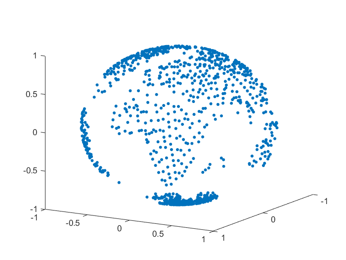
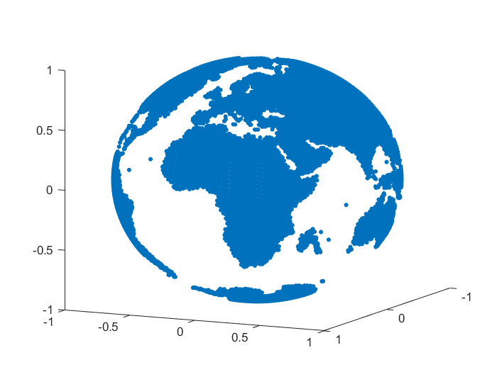
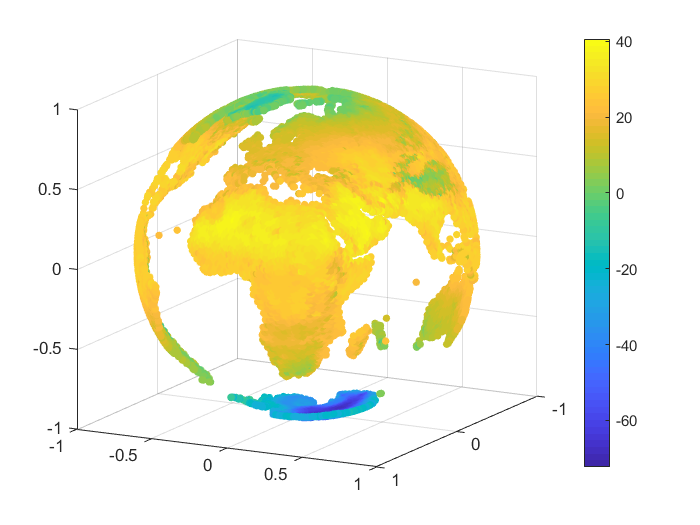
We consider an example of approximation for some real data, namely the monthly-mean temperatures on the Globe in January 2010 and June 2010. The set of data was selected from [28]. For our numerical tests we considered $1073$ nodes and we reconstructed the temperature values for $21449$ points on the Globe, after we projected the latitude and longitude of each point onto the unit sphere $S$ . A representation for the sets of nodes and points is given in Figure 3.

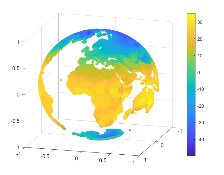
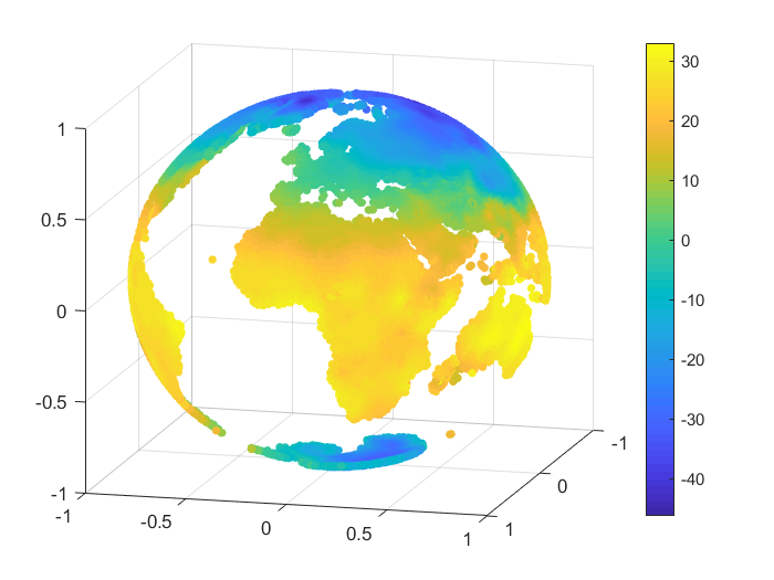
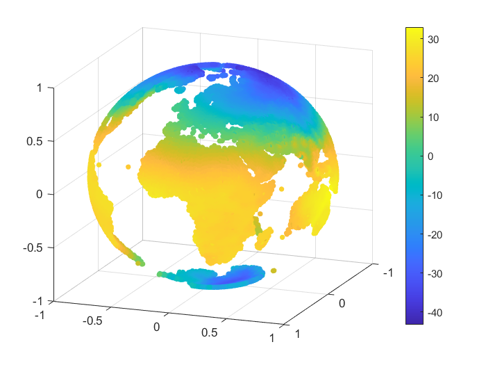
To handle the global part, we considered the case of zonal basis functions combined with a spherical harmonic, $S_{2}$ and $S_{4}$ . For the inverse multiquadric case, we computed the parameter $c$ as in the previous numerical tests (see, e.g., [18]). The value obtained was $c=35.26$ . In Table 12 there are given the mean absolute errors (MAEs) and the root mean square errors (RMSEs). Figures 4, 5 present the graphical results for the temperatures in January 2010 and June 2010, respectively. Studying the results obtained for this example, there are observed and confirmed the advantages of using the previously introduced combined Shepard operators to real data applications.

	January		June
	$S_{2}$	$S_{4}$	$S_{2}$	$S_{4}$
MAE	$2.08^{\circ}C$	$2.63^{\circ}C$	$2.11^{\circ}C$	$2.75^{\circ}C$
RMSE	$5.31^{\circ}C$	$7.61^{\circ}C$	$5.09^{\circ}C$	$7.81^{\circ}C$

Table 12. Errors for mean global temperatures in

January 2010 and June 2010.

Data availability. All data generated or analysed during this study are included in this published article.

Conflict of interest. The authors have no conflict of interests to declare that are relevant to the content of this article.

Ethical Approval. Not applicable.

Availability of supporting data. Not applicable.

Competing interests. Not applicable.

Funding. Not applicable.

Authors’ contributions. Equal contributions.

Acknowledgments. We are grateful to the referees for the careful reading and for their valuable suggestions that improved the manuscript.

References

[1] Allasia, G., Cavoretto, R., De Rossi, A.: Hermite-Birkhoff interpolation on scattered data on the sphere and other manifolds. Appl. Math. Comput. 318, 35–50 (2018)
[2] Baxter, B.J.C., Hubbert, S.: Radial basis functions for the sphere. In: Recent Progress in Multivariate Approximation, Witten-Bommerholz, 2000. Internat. Ser. Numer. Math., vol. 137, pp. 33–47. Birkhäuser, Basel (2001)
[3] Cătinaş, T.: The combined Shepard-Abel-Goncharov univariate operator. Rev. Anal. Numér. Théor. Approx. 32, 11–20 (2003)
[4] Cătinaş, T.: The combined Shepard-Lidstone bivariate operator. In: Trends and Applications in Constructive Approximation. International Series of Numerical Mathematics (de Bruin, M.G. et al. (eds.)), 151, pp. 77–89, Springer Group-Birkhäuser Verlag (2005)
[5] Cătinaş, T.: Bivariate interpolation by combined Shepard operators. In: Proceedings of $17^{th}$ IMACS World Congress, Scientific Computation, Applied Mathematics and Simulation (Borne, P., Benrejeb, M., Dangoumau, N., Lorimier, L. (eds.)), 7 pp., Paris, July 11–15 (2005)
[6] Cătinaş, T.: The bivariate Shepard operator of Bernoulli type. Calcolo 44(4), 189–202 (2007)
[7] De Rossi, A.: Spherical interpolation of large scattered data sets using zonal basis functions. In: Mathematical Methods for Curves and Surfaces (Daehlen, M., Morken, K., Schumaker, L. (eds.)), pp. 125–134, Trømso 2004. Nashboro Press (2005)
[8] De Rossi, A.: Hybrid spherical approximation. arXiv:1404.1475 (2014)
[9] Cavoretto, R., De Rossi, A.: Fast and accurate interpolation of large scattered data sets on the sphere. J. Comput. Appl. Math. 234, 1505–1521 (2010)
[10] Cavoretto, R., De Rossi, A.: Numerical comparison of different weights in Shepard’s interpolants on the sphere. Appl. Math. Sci. 4, 3425–3435 (2010)
[11] Cavoretto, R., De Rossi, A.: Spherical interpolation using the partition of unity method: An efficient and flexible algorithm. Appl. Math. Lett. 25, 1251–1256 (2012)
[12] Cavoretto, R., De Rossi, A.: Achieving accuracy and efficiency in spherical modelling of real data. Math. Methods Appl. Sci. 37, 1449–1459 (2014)
[13] Farwig, R.: Rate of convergence of Shepard’s global interpolation formula. Math. Comp. 46, 577–590 (1986)
[14] Fasshauer, G.E., Zhang J.G.: On choosing “optimal” shape parameters for RBF approximation. Numer. Algor. 45, 345–368 (2007)
[15] Franke, R.: Scattered data interpolation: tests of some methods. Math. Comp. 38, 181–200 (1982)
[16] Franke, R., Nielson, G.: Smooth interpolation of large sets of scattered data. Int. J. Numer. Meths. Engrg. 15, 1691–1704 (1980)
[17] Le Gia, Q.T., Sloan, I. H., Wendland, H.: Multiscale analysis in Sobolev spaces on the sphere. SIAM J. Numer. Anal. 48(6), 2065–2090 (2010)
[18] Hardy, R.L.: Multiquadric equations of topography and other irregular surfaces. J. Geophys. Res. 76, 1905–1915 (1971)
[19] Hubbert, S., Le Gia, Q.T., Morton, T.: Spherical Radial Basis Functions, Theory and Applications. Springer (2015)
[20] Lazzaro, D., Montefusco, L.B.: Radial basis functions for multivariate interpolation of large scattered data sets. J. Comput. Appl. Math. 140, 521–536 (2002)
[21] Renka, R.J., Cline, A.K.: A triangle-based $C^{1}$ interpolation method. Rocky Mountain J. Math. 14, 223–237 (1984)
[22] Renka, R.J.: Multivariate interpolation of large sets of scattered data. ACM Trans. Math. Software 14, 139–148 (1988)
[23] Saff, E.B., Kuijlaars, A.B.J.: Distributing many points on a sphere. Math. Intelligencer. 19, 5–11 (1997)
[24] Shepard, D.: A two dimensional interpolation function for irregularly spaced data. In: Proceedings of the 1968 23rd ACM National Conference, pp. 517–523. ACM (1968)
[25] Sloan, I.H., Sommariva, A.: Approximation on the sphere using radial basis functions plus polynomials. Adv. Comput. Math., 29, 147–177 (2008)
[26] Wong, T.T., Luk, W.S., Heng, P.A.: Sampling with Hammersley and Halton Points. J. Graph. Tools, 2(2), 9-24 (1997)
[27] Zuppa, C.: Error estimates for moving least square approximations. Bull. Braz. Math. Soc. (N.S), 34(2), 231–249 (2003)
[28] https://www.kaggle.com/datasets/shishu1421/global-temperature?select=air_temp.2010

[1] Allasia, G., Cavoretto, R., De Rossi, A., Hermite-Birkhoff interpolation on scattered data on the sphere and other manifolds. Appl. Math. Comput. 318, 35–50 (2018), MathSciNet Google Scholar

[2] Baxter, B.J.C., Hubbert, S., Radial basis functions for the sphere. In: Recent Progress in Multivariate Approximation, Witten-Bommerholz, 2000. Internat. Ser. Numer. Math., vol. 137, pp. 33-47. Birkhäuser, Basel (2001)

[3] Cătinaş, T., The combined Shepard-Abel-Goncharov univariate operator. Rev. Anal. Numér. Théor. Approx. 32, 11–20 (2003), Article Google Scholar

[4] Cătinaş, T., The combined Shepard-Lidstone bivariate operator. In: Trends and Applications in Constructive Approximation. International Series of Numerical Mathematics (de Bruin, M.G. et al. (eds.)), 151, pp. 77–89, Springer Group-Birkhäuser Verlag (2005)

[5] Cătinaş, T., Bivariate interpolation by combined Shepard operators. In: Proceedings of 17^{th} $17^{t h}$ IMACS World Congress, Scientific Computation, Applied Mathematics and Simulation (Borne, P., Benrejeb, M., Dangoumau, N., Lorimier, L. (eds.)), 7 pp., Paris, July 11–15 (2005)

[6] Cătinaş, T., The bivariate Shepard operator of Bernoulli type. Calcolo 44(4), 189–202 (2007), Article MathSciNet Google Scholar

[7] De Rossi, A., Spherical interpolation of large scattered data sets using zonal basis functions. In: Mathematical Methods for Curves and Surfaces (Daehlen, M., Morken, K., Schumaker, L. (eds.)), pp. 125–134, TrØmso 2004. Nashboro Press (2005)

[8] De Rossi, A., Hybrid spherical approximation. arXiv:1404.1475 (2014)

[9] Cavoretto, R., De Rossi, A., Fast and accurate interpolation of large scattered data sets on the sphere. J. Comput. Appl. Math. 234, 1505–1521 (2010), Article MathSciNet Google Scholar

[10] Cavoretto, R., De Rossi, A., Numerical comparison of different weights in Shepard’s interpolants on the sphere. Appl. Math. Sci. 4, 3425–3435 (2010), MathSciNet Google Scholar

[11] Cavoretto, R., De Rossi, A., Spherical interpolation using the partition of unity method: an efficient and flexible algorithm. Appl. Math. Lett. 25, 1251–1256 (2012), Article MathSciNet Google Scholar

[12] Cavoretto, R., De Rossi, A., Achieving accuracy and efficiency in spherical modelling of real data. Math. Methods Appl. Sci. 37, 1449–1459 (2014), Article MathSciNet Google Scholar

[13] Farwig, R., Rate of convergence of Shepard’s global interpolation formula. Math. Comp. 46, 577–590 (1986), MathSciNet Google Scholar

[14] Fasshauer, G.E., Zhang, J.G., On choosing “optimal’’ shape parameters for RBF approximation. Numer. Algor. 45, 345–368 (2007), Article MathSciNet Google Scholar

[15] Franke, R., Scattered data interpolation: tests of some methods. Math. Comp. 38, 181–200 (1982), MathSciNet Google Scholar

[16] Franke, R., Nielson, G., Smooth interpolation of large sets of scattered data. Int. J. Numer. Meths. Engrg. 15, 1691–1704 (1980), Article MathSciNet Google Scholar

[17] Le Gia, Q.T., Sloan, I.H., Wendland, H., Multiscale analysis in Sobolev spaces on the sphere. SIAM J. Numer. Anal. 48(6), 2065–2090 (2010), Article MathSciNet Google Scholar

[18] Hardy, R.L., Multiquadric equations of topography and other irregular surfaces. J. Geophys. Res. 76, 1905–1915 (1971), Article Google Scholar

[19] Hubbert, S., Le Gia, Q.T., Morton, T., Spherical radial basis functions. Springer, Theory and Applications (2015), Book Google Scholar

[20] Lazzaro, D., Montefusco, L.B., Radial basis functions for multivariate interpolation of large scattered data sets. J. Comput. Appl. Math. 140, 521–536 (2002), Article MathSciNet Google Scholar

[21] Renka, R.J., Cline, A.K., A triangle-based C¹ $C^{1}$ interpolation method. Rocky Mountain J. Math. 14, 223–237 (1984), Article MathSciNet Google Scholar

[22] Renka, R.J., Multivariate interpolation of large sets of scattered data. ACM Trans. Math. Software 14, 139–148 (1988), Article MathSciNet Google Scholar

[23] Saff, E.B., Kuijlaars, A.B.J., Distributing many points on a sphere. Math. Intelligencer. 19, 5–11 (1997), Article MathSciNet Google Scholar

[24] Shepard, D., A two dimensional interpolation function for irregularly spaced data. In: Proceedings of the 1968 23rd ACM National Conference, pp. 517–523. ACM (1968)

[25] Sloan, I.H., Sommariva, A., Approximation on the sphere using radial basis functions plus polynomials. Adv. Comput. Math. 29, 147–177 (2008), Article MathSciNet Google Scholar

[26] Wong, T.T., Luk, W.S., Heng, P.A., Sampling with Hammersley and Halton Points. J. Graph. Tools 2(2), 9–24 (1997), Article Google Scholar

[27] Zuppa, C.: Error estimates for moving least square approximations. Bull. Braz. Math. Soc. (N.S) 34(2), 231–249 (2003), Article MathSciNet Google Scholar

2024

Recovering and posting started for the older annual reports, 1951-1989

8 Feb at 10:01 am

Properties of positive linear operators connected with squared fundamental functions

11 Mar at 7:41 am

Testing Weyl geometric gravity with the SPARC galactic rotation curves database

12 Feb at 10:52 am

	$\displaystyle E_{i}(\mathbf{x})$	$\displaystyle=\left\|f(\mathbf{x})-S_{i}(\mathbf{x})\right\|=\left\|f(\mathbf{x})% \cdot 1-\sum\limits_{j=1}^{n}\overline{w}_{j}(\mathbf{x})Z_{j}^{(i)}(\mathbf{x% })\right\|$
		$\displaystyle=\left\|f(\mathbf{x})\sum\limits_{j=1}^{n}\overline{w}_{j}(\mathbf% {x})-\sum\limits_{j=1}^{n}\overline{w}_{j}(\mathbf{x})Z_{j}^{(i)}(\mathbf{x})% \right\|=\left\|\sum\limits_{j=1}^{n}\overline{w}_{j}(\mathbf{x})\left[f(x)-Z_{j% }^{(i)}(\mathbf{x})\right]\right\|$
		$\displaystyle\leq\sum\limits_{j=1}^{n}\left\|\overline{w}_{j}(\mathbf{x})\left[% f(\mathbf{x})-Z_{j}^{(i)}(\mathbf{x})\right]\right\|=\sum\limits_{j=1}^{n}% \overline{w}_{j}(\mathbf{x})\left\|f(\mathbf{x})-Z_{j}^{(i)}(\mathbf{x})\right\|$
		$\displaystyle=\sum\limits_{j=1}^{n}\overline{w}_{j}(\mathbf{x})e_{j}(\mathbf{x% }),\mbox{ for each }i=1,...,4,\mbox{ and each }\mathbf{x}\in S.$

	$\displaystyle\|S_{i}(\mathbf{x})-f(\mathbf{x})\|$	$\displaystyle=\left\|\sum\limits_{j=1}^{n}\overline{w}_{j}(\mathbf{x})\cdot Z_{% j}^{(i)}(\mathbf{x})-f(\mathbf{x})\cdot\sum\limits_{j=1}^{n}\overline{w}_{j}(% \mathbf{x})\right\|=\left\|\sum\limits_{j=1}^{n}\overline{w}_{j}(\mathbf{x})% \cdot[Z_{j}^{(i)}(\mathbf{x})-f(\mathbf{x})]\right\|$
		$\displaystyle=\left\|\sum\limits_{j=1}^{n}\overline{w}_{j}(\mathbf{x})\cdot[Z_{% j}^{(i)}(\mathbf{x})-f(\mathbf{x}_{j})+f(\mathbf{x}_{j})-f(\mathbf{x})]\right\|$
		$\displaystyle\leq\sum\limits_{j=1}^{n}\overline{w}_{j}(\mathbf{x})\cdot\|Z_{j}^% {(i)}(\mathbf{x})-f(\mathbf{x}_{j})\|+\sum\limits_{j=1}^{n}\overline{w}_{j}(% \mathbf{x})\cdot\|f(\mathbf{x}_{j})-f(\mathbf{x})\|$
		$\displaystyle\leq\sum\limits_{j=1}^{n}\overline{w}_{j}(\mathbf{x})\cdot\|Z_{j}^% {(i)}(\mathbf{x})-Z_{j}^{(i)}(\mathbf{x}_{j})\|+\omega(f,h_{X}),\ \ i=1,...,4.$

Spherical interpolation of scattered data using least squares thin-plate spline and inverse multiquadric functions

Abstract

Authors

Keywords

Paper coordinates

PDF

About this paper

Journal

Publisher Name

DOI

Print ISSN

Online ISSN

Paper (preprint) in HTML form

Spherical interpolation of scattered data using least squares thin-plate spline and inverse multiquadric functions

Abstract.

1. Preliminaries

2. Combined spherical Shepard method

Definition 2.1.

Definition 2.2.

Definition 2.3.

Definition 2.4.

Definition 2.5.

Definition 2.6.

Remark 2.7.

Remark 2.8.

Theorem 2.9.

Proof.

Theorem 2.10.

Proof.

Theorem 2.11.

Proof.

3. Test results

References

References

Related Posts

Spherical interpolation of scattered data using
least squares thin-plate spline and
inverse multiquadric functions