Abstract
In this paper we introduce a Stancu-Schurer type extension of higher order of the Cheney-Sharma operators. Starting from the operators studied by Bostanci and Ba\c scanbaz-Tunca, respectively by C\u atina\c s and Buda (in the form of a Stancu operator with generalized Bernstein polynomials) we extend the convex combination of two terms which appears in the expression of the operator to a convex combination of $m$ terms, where $m\in\mathbb{N}$, with $m\geq 1$. We called these new operators the Stancu-Schurer type extension of order $m$ of the Cheney-Sharma operators (of first, respectively second kind). For these operators we study some approximation and convexity properties, modulus of continuity and Korovkin-type theorems.
Authors
Eduard Stefan Grigoriciuc
Faculty of Mathematics and Computer Science, Babeş-Bolyai University, Cluj-Napoca, Romania
Tiberiu Popoviciu Institute of Numerical Analysis, Romanian Academy, Cluj-Napoca, Romania
Andra Malina
Faculty of Mathematics and Computer Science, Babeş-Bolyai University, Cluj-Napoca, Romania
Tiberiu Popoviciu Institute of Numerical Analysis, Romanian Academy, Cluj-Napoca, Romania
Keywords
Cheney-Sharma operator, Stancu-Schurer operator, Jensen inequality, modulus of continuity, Korovkin theorem
Paper coordinates
E.S. Grigoriciuc, A. Malina, A Stancu-Schurer type extension of higher order of the Cheney-Sharma operators, Math. Slovaca (2026), to appear (DOI: 10.1515/ms-2025-1155)
??
About this paper
Print ISSN
1337-2211
Online ISSN
google scholar link
Paper (preprint) in HTML form
A Stancu-Schurer type extension of higher order of the Cheney-Sharma operators
Abstract.
In this paper we introduce a Stancu-Schurer type extension of higher order of the Cheney-Sharma operators. Starting from the operators studied by Bostanci and Başcanbaz-Tunca, respectively by Cătinaş and Buda (in the form of a Stancu operator with generalized Bernstein polynomials) we extend the convex combination of two terms which appears in the expression of the operator to a convex combination of terms, where , with . We called these new operators the Stancu-Schurer type extension of order of the Cheney-Sharma operators (of first, respectively second kind). For these operators we study some approximation and convexity properties, modulus of continuity and Korovkin-type theorems.
Key words and phrases:
Cheney-Sharma operator, Stancu-Schurer operator, Jensen inequality, modulus of continuity, Korovkin theorem2010 Mathematics Subject Classification:
Primary 41A35, 41A36, 47A581. Introduction
For and , Bernstein introduced in [6] the following linear and positive operators
| (1.1) |
with the basis polynomials given by
| (1.2) |
for , and . Later on, using a probabilistic approach, Stancu introduced in [29] another type of linear and positive operators, defined as
| (1.3) |
with the polynomials given by (1.2), , and a non-negative integer such that , for every .
Over time, various generalizations of this operator have been made. Among the generalized operators that have been introduced and studied, we mention here only the Bernstein-Stancu operator (see e.g. [28]), the Stancu-Schurer operator (see e.g [21], [25]), the Brass-Stancu operator (see e.g. [8] and [10]), the Stancu-Kantorovich operator (see e.g. [18]). In each of these generalizations (as well as in others studied but not mentioned here), the fundamental polynomials are multiplied by values of the function , respectively linear combinations of values of the function . The novelty of the generalization presented in this paper consists in the use of higher-order combinations, as can be seen in the following definition.
Definition 1.
Consider , . Also, let be such that , where . Then, for every function , we define the generalized Stancu operator of order by
| (1.4) |
where the polynomials are given by (1.2).
In order to generalize the previous operator, a small modification can be made in its definition. Similarly to what was done in [25] (see also [16], [24]), we consider with and the space of continuous functions in the interval .
Remark 1.
It is not difficult to observe that is the classical Stancu operator (of order one) defined by (1.3) and is the classical Stancu-Schurer operator defined in [25].
Remark 2.
Using the above notations, the Cheney-Sharma operator of the first kind is given as (see [19])
| (1.10) |
while the Cheney-Sharma operator of the second kind is defined as (see [19])
| (1.11) |
for any function . Note that, recently, the Cheney-Sharma operators have been studied on different domains in higher dimensions. In [11] and [12] the authors present some extensions of these operators on a triangle with straight sides, respectively with one curved side. Other properties on such domains are studied in [14] and [15] in terms of iterates of multivariate Cheney-Sharma type operators.
Lemma 1.1.
We end this introductory section by bringing together already known results and innovative ideas that open the way for the study of the operators introduced in this paper. The primary elements that we will use in the construction of the new operators are the generalized Stancu-Schurer operator of order given by (1.5) and the Cheney-Sharma polynomials and given by (1.8), respectively by (1.9).
Using these types of operators, respectively, basis polynomials, we can construct a new generalization of the Stancu-Schurer and Cheney-Sharma operators. Taking into account that Cheney and Sharma defined two types of operators, i.e., of the first, respectively the second kind, we can define the Stancu-Schurer type extension of order for both cases. These two operators will be defined and rigorously studied in the following sections.
In Section 2 we present the definitions of our new operators, denoted by , respectively , where with and . The next two sections are dedicated to the study of the operator . In Section 3 we include some properties related to the moments, approximation and convexity of the operator . On the other hand, in Section 4 we discuss Korovkin-type theorems for the same operator . Finally, Section 5 contains some results related to the operator , less studied in this paper, but which will be addressed in a subsequent study. The paper ends with a section of conclusions and further research directions.
2. Extensions of higher orders of the Cheney-Sharma operators
In this section, based on the ideas presented above, we construct new operators of Cheney-Sharma type, considering a Stancu-Schurer extension of higher order. Particular cases of the operators introduced in this section have been studied by Bostanci and Başcanbaz-Tunca in [7], respectively by Cătinaş and Buda in [13]. Hence, inspired by the results obtained in the foundational work of Bostanci and Başcanbaz-Tunca and also Cătinaş and Buda we study some general properties of our newly formulated operators.
For these operators, moment calculations, approximation and convexity properties are studied (see Section 3, respectively Section 5). In addition, for the Stancu-Schurer type extension of order of the second Cheney-Sharma operator we study the modulus of continuity and prove some relevant Korovkin-type results (see Section 4).
Definition 2.
Consider , and . Let be such that , where . Then, for every continuous function , we define:
It is clear that is the generalized Stancu-Schurer operator of order defined by (1.5). Moreover, if and , then and are the Stancu type extensions of the Cheney-Sharma operators of the first (respectively, the second) kind studied by Cătinaş and Buda in [13], respectively by Bostanci and Başcanbaz-Tunca in [7].
In addition, one can easily see that if and , then and are the Cheney-Sharma operators of the first and second kind, respectively, given in (1.10) and (1.11), respectively, both reducing to the Bernstein operator (1.2) when .
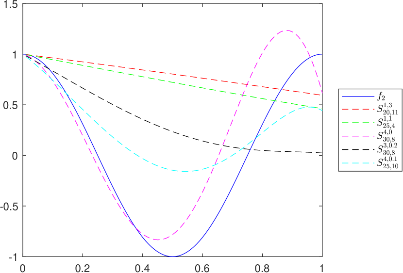
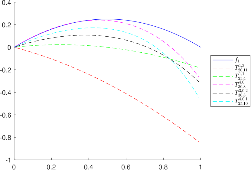
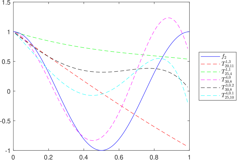
Example 1.
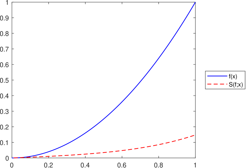
To graphically illustrate the operators and , given in (2.1) and (2.2), respectively, we consider the functions (see e.g. [8])
The graphs of the functions and , together with those of the corresponding operators and , are presented in Figures 1 and 2, respectively, for several choices of the parameters appearing in the definitions of the operators.
3. Properties of the operator
In this section we focus our attention on the properties of the second-type extension operator . We study the expressions of the moments of and some properties related to them. Finally, we study approximation and convexity results. The proofs of our results follow the ideas presented in [30] (see also [7], [19] and [22]) for the particular case .
3.1. Moments of and their properties
Theorem 3.1.
Consider , and . Let be such that , where . Also, let , for every and . Then
-
a)
;
-
b)
, for .
In particular, , for all .
Proof.
Following the ideas presented in [30] (see also [7] and [22]), we can give a complete proof of the previous two relations.
- a)
-
b)
For the second case, let , for all . Also, for simplicity, let us denote by . Then
in view of the first part of this result, where we denoted by
(3.1) Since the first term of the sum is zero, we obtain that
Next, let us denote . Then B_λ(x)=λn ∑_j=0^λ-1(λ-1 j) x[x+(j+1)β]j(1-x)[1-x+(λ-j-1) β]λ-j-2(1+ λβ)λ-1. If we denote the index of summation by and take into account that x+(k+1)β=(1+λβ)-[1-x+(λ-k-1)β], then
according to relation (1.7) for , and . Finally, we obtain that
where and this completes the proof.
∎
Remark 3.
It is clear that , for every , where is replaced by , respectively by in formula (1.11). Hence, the previous proof can be particularized for the Cheney-Sharma operator (see [19]). Indeed, if , then Theorem 3.1 reduces to the results obtained by Cheney and Sharma in [19], respectively by Bostanci and Başcanbaz-Tunca in [7] (see Lemma 1.1).
Remark 4.
For all and any , we can prove the following immediate properties:
-
a)
;
-
b)
. In particular, if , then .
Lemma 3.1.
Consider , and . Let be such that , where . If , then
| (3.2) |
where , for all . The equality holds if and only if .
Proof.
According to Theorem 3.1, we know that
where . If , then the inequality (3.2) is obvious, since and .
Next, let us consider such that . Simple computations show then that (3.2) is equivalent to
| (3.3) |
where , and . In order to obtain the inequality (3.3), it is sufficient that all the coefficients of be non-negative, i.e., and , but this is true in view of our hypothesis. Hence, , for all and this completes the proof. ∎
Lemma 3.2.
Consider , and . Let be such that , where . If and , then
| (3.4) |
where , for all .
Proof.
Remark 5.
Next, we state an auxiliary result (see [7, Lemma 2.1]), which we shall use in the sequel.
Lemma 3.3.
Following the ideas presented by Cheney and Sharma in [19] (see also [7]), we can prove the following result related to the expression of on .
Theorem 3.2.
Consider , and . Let be such that , where . Also, let , for every and . Then
where is given by the formula
| (3.9) |
for all and with
| (3.10) |
and
| (3.11) |
Next, we give a detailed proof of the previous result. A sketch of the ideas used in this proof has been presented in [19] (see also [7]).
Proof.
Let , for all . Then
For simplicity, let us denote by and by . Then
According to the proof of Theorem 3.1 we have that
where (see the first part of Theorem 3.1), is given by (3.1) and
| (3.12) |
for all . The next important step in our proof is to compute the expression of given by (3.12). We have that
It is not difficult to observe that the second sum reduces to , where is given by (3.1) and then
Moreover,
If we compute separately the sum in the last member of the previous equality, we obtain
where we replaced by . According to Lemma 3.3, the expression on the right hand side of the previous equality reduces to given by (3.6). Hence,
Based on relation (3.8) for , and , we have that
Finally, if we denote
and
then
and this completes the proof. ∎
Remark 6.
If , then , hence , for any .
Another important result presented in this section explores the norm of the operator applied on a continuous function defined on the interval .
Proposition 3.3.
For every , we have that
where denotes the uniform norm on the space .
3.2. Convexity properties of the operator
Inspired by the property presented in [26, Theorem 3] (see also [5, Theorem 3] and [22, Proposition 12]), we can prove an important result related to the operator . Although the inequality relation does not apply to , it nevertheless generalizes the results obtained for other operators (for example, if and , then Proposition 3.4 reduces to [22, Proposition 12] for the extremal case ).
Proposition 3.4.
If is convex on , then , for all .
Proof.
Based on (2.2), we have that:
For simplicity of notation, we denote by with and by . The operator can now be written as
Hence,
| (3.13) |
for all . ∎
Remark 7.
Proposition 3.5.
If and is an increasing convex function on , then , for all .
Proof.
In view of Propostion 3.4 we know that if is convex on , then
| (3.14) |
Since is increasing on , it follows that for any two points with we have that . In particular, for and , we know (see Lemma 3.1) that
for all . Hence,
| (3.15) |
In view of relations (3.14) and (3.15) we deduce that , for all and this completes the proof. ∎
Remark 8.
It is important to observe that the convexity property imposed in Proposition 3.5 is essential in order to obtain the inequality , for all . To illustrate this fact, let us consider the following example in which the function is not convex on its domain.
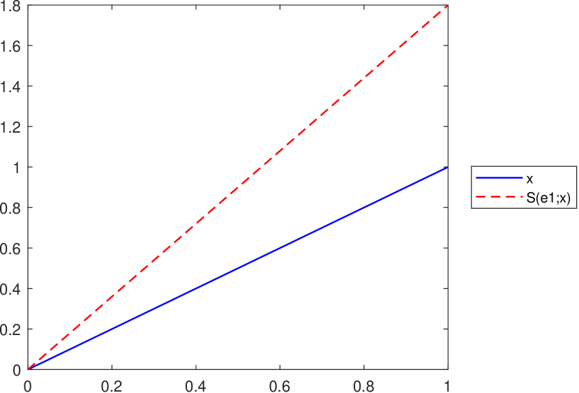
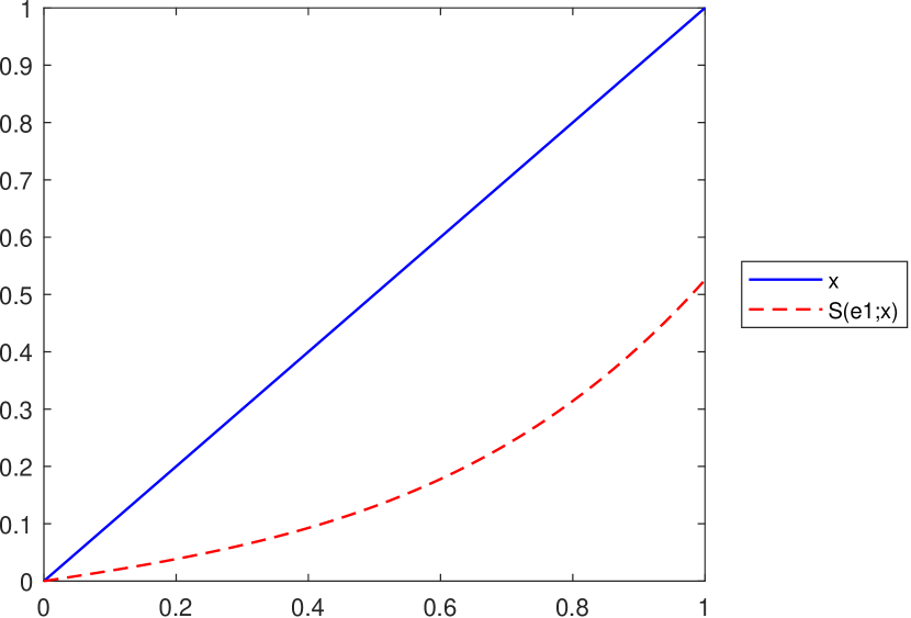
Example 2.
Let be given by , for all . Since is not convex on , we obtain the following counterexamples of Proposition 3.5:
-
•
Let . According to Lemma 3.1 and Remark 5 we know that , for all . However, since is not convex on , we have that , for all , as it can be observed in Figure 4 and Figure 4.
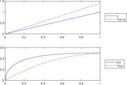
Figure 3. , , , and . 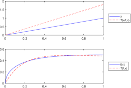
Figure 4. , , , and . -
•
Let . In this case, , for all only if (see Lemma 3.1). Although this condition can be easily fulfilled by choosing a suitable number , since the function is not convex, we do not obtain the inequality from Proposition 3.5. This important remark is illustrated in Figure 6, respectively in Figure 6. In each case we consider , , , , , and .
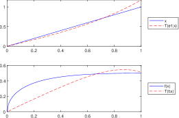
Figure 5. . 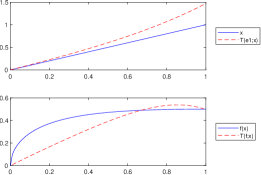
Figure 6. .
Similar examples can be obtained for different values of constants , and non-convex functions defined on .
4. Korovkin type theorems for the operator
In this section we study some approximation results based on the modulus of continuity and show that the operator satisfies the conditions of the Korovkin-type theorem (see [3], [20], [27], [31]). In order to prove the first result of this section, we introduce the following auxiliary lemma.
Lemma 4.1.
[31]
Considering and the modulus of continuity associated to ,
, there exists a positive constant such that
| (4.1) |
where is given as
with and .
We can now prove the following result.
Theorem 4.1.
Consider , and . Let be such that , where , with . If we denote by
and by
then
Proof.
Since the operator is linear, we have that
Now, using Proposition 3.3, we obtain
| (4.2) |
Since , applying Lagrange theorem, we have that there exists a point between and such that
Applying the linear operator , we get
and for
Substituting this into (4.2), we obtain
Taking the infimum over all , by relation (4.1), we get that
which completes the proof. ∎
Theorem 4.2.
If , the operator satisfies the following relation
| (4.3) |
5. Properties of the operator
In this section we direct our attention to the first-type extension operator . As for the previous operator, we study the expressions of the moments and some approximation results. Although not all the properties of the operator carry over directly to , as shown in this section through some examples, several others can be established for .
Theorem 5.1.
Consider , and . Let be such that , where and denote by . Also, let , for every and . Then
-
a)
;
-
b)
, where
(5.1) - c)
Proof.
- a)
- b)
-
c)
Following the ideas of the proof of Theorem 3.2, we have that S^m,β_n,p(e_2;x) = 1n2 (r_1^2 x + r_2^2 x^2 + …+ r_m^2 x^m ) + 2 λ(r1x + r2x2+ …rmxm)n2 ~M_λx + ~C_λ(x), with
(5.6) Applying now a result presented in [13, Lemma 3], we have that ∑_k=0^λ k2λ2 a_λ.k^β(x) = λ-1λ [x(x+2 β) ~A_λ + x(λ-2)β^2 ~B_λ ] + 1λ ~M_λx, hence ~C_λ(x) = λ(λ-1)n2 [x(x+2 β) ~A_λ + x(λ-2)β^2 ~B_λ ] + λn2 ~M_λx, with , and given in (5.3), (5.4) and (5.1), respectively.
∎
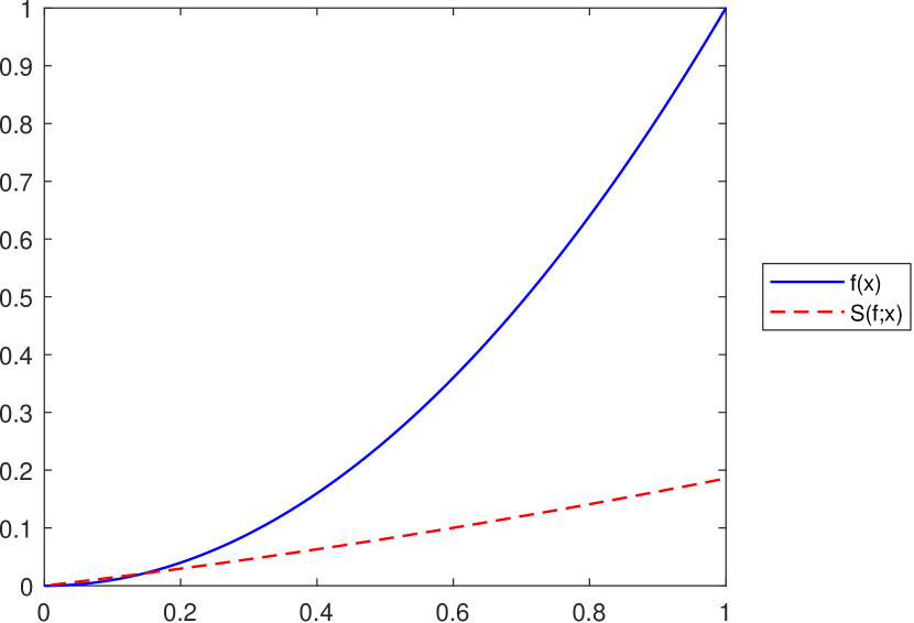
Remark 9.
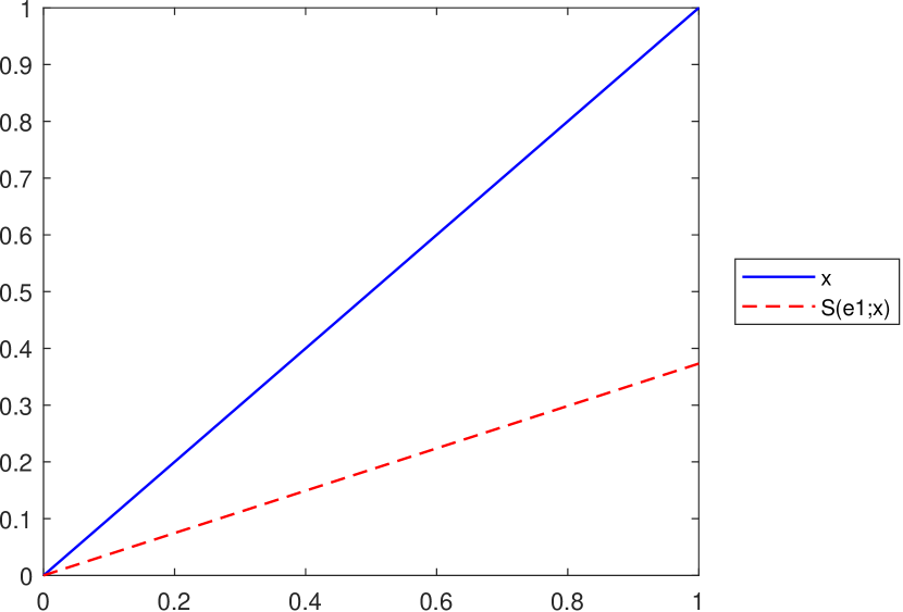
As pointed out in Lemma 3.1, the inequality , for all is satisfied if , where and . However, in the case of the operator this is not always true, as illustrated in Figure 7.
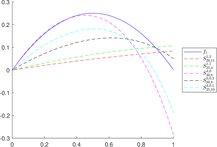
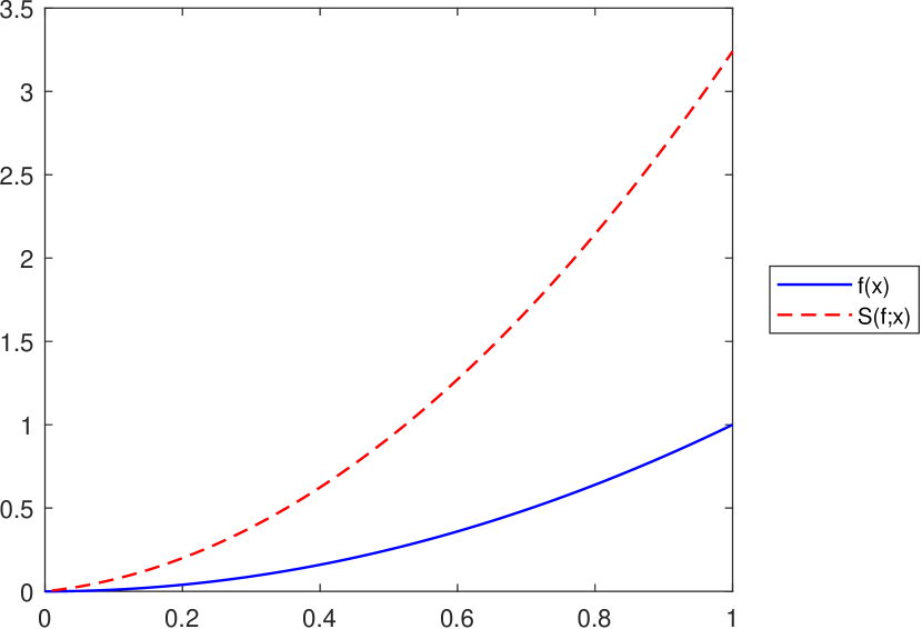
Remark 10.
As mentioned at the end of Section 4, the operator does not satisfy an inequality of the form for all , with being an increasing convex function on , as was proved in Proposition 3.5 for the operator . This is illustrated in Figure 8, considering the function on and various values for the operator’s parameters.
Remark 11.
If , then , hence and we can apply a Korovkin-type result as in Theorem 4.2 for the operator .
Proposition 5.2.
For every , we have that
where denotes the uniform norm on the space .
Proof.
It is similar to the result proven in Proposition 3.3. ∎
6. Conclusions and future work
We end this paper with a short comparative analysis of the operators and with analogous operators presented in the literature. We will point out the main distinctions and possible advantages of the operators introduced in this paper. It is clear that the closest family of operators is that of shifted-knot Bernstein-Stancu operators (the classical generalization where the evaluation nodes and weights are shifted by parameters). However, in our case, the operators use multiple shifts with different weights . Moreover, the weighted combination depends on powers of , and this gives us more flexibility and local adaptation. Our operators remain in the Bernstain-Stancu family, but enrich it via multiple shifts and weighted combination of evaluations, without changing to an integral-based or multivariate framework. In contrast with Bernstein-Stancu operators with shifted knots (see e.g. [1], [4], [23], [32]), Baskakov-Kantorovich operators (see e.g. [9], [33]), or Baskakov-Schurer-Stancu generalizations that use single shifts (see e.g. [2], [9]), the operators introduced in this paper stand out by using multiple shifted evaluations per basis node, weighted by powers of . Again, this particular property offers more local flexibility and adjusatable approximation at different regions through .
It is clear that other important properties can be obtained for the operators , respectively in (e.g., the preservation of the Lipschitz property, extensions of Chlodovsky type, the case of three parameters, the multivariate case of the Cheney-Sharma operators). Different extensions and results were recently obtained by Başcanbaz-Tunca in [4], Başcanbaz-Tunca, Erençin and Taşdelen in [5] and [32], Miclăuş in [24], or Söylemez and Taşdelen in [26] and [27]. An interesting problem would be to study how such results can be adapted or generalized to the operators introduced in our paper.
On the other hand, Çetin and Mutlu have recently obtained extensions of the classical results in the complex plane (see [16] and [17]). Taking into account their ideas, it will be of interest to prove similar results for and in (extension results and preservation of geometric properties of the original function such as univalence, starlikeness, convexity and spirallikeness).
Acknowledgments
The authors thank the referees for carefully reading the manuscript and providing helpful suggestions.
References
- [1] AGRATINI, O.: Stancu modified operators revisited, Rev. Anal. Numér. Théor. Approx. 31(1), 9–16, 2002.
- [2] AGRAWALA, P.N.—GOYALA, M.: Generalized Baskakov Kantorovich Operators Filomat 31(19), 6131–6151, 2017.
- [3] ALTOMARE, F.—CAMPITI, M.: Korovkin-type approximaton theory and its applications, Walter de Gruyter, Berlin-New York, 1994.
- [4] BAŞCANBAZ-TUNCA, G.: A note on Stancu operators with three parameters, Bull. Transilv. Univ. Braşov Ser. III. Math. Comput. Sci. 5(67), 55–70, 2025.
- [5] BAŞCANBAZ-TUNCA, G.—ERENÇIN, A.—TAŞDELEN, F.: Some properties of Bernstein type Cheney and Sharma operators, General Mathematics 24(1-2), 17–25, 2016.
- [6] BERNSTEIN, S.N.: Démonstration du théoréme de Weierstrass fondée sur le calcul des probabilités, Commun. Kharkov Math. Soc. 13, 1–2, 1912/1913.
- [7] BOSTANCI, T.—BAŞCANBAZ-TUNCA, G.: A Stancu type extension of Cheney and Sharma operator, J. Numer. Anal. Approx. Theory 47(2), 124–134, 2018.
- [8] BODUR, M.—BOSTANCI, T., BAŞCANBAZ-TUNCA, G.: On Kantorovich variant of Brass-Stancu operators Demonstratio Mathematica 57(1), pp. 20240007, 2024.
- [9] BUSTAMANTE, J.: Baskakov-Kantorovich operators reproducing affine functions Stud. Univ. Babeş-Bolyai Math. 66(4), 739–756, 2021.
- [10] BRASS, H.: Eine Verallgemeinerung der Bernsteinschen Operatoren Abh. Math. Sem. Univ. Hamburg 38, 111–122. 1971.
- [11] CĂTINAŞ, T.: Extension of some Cheney-Sharma type operators to a triangle with one curved side, Miskolc Math. Notes 21, 101–111, 2020.
- [12] CĂTINAŞ, T.: Cheney–Sharma type operators on a triangle with straight sides, Symmetry 14(11), 2446, 2022.
- [13] CĂTINAŞ, T.—BUDA, I.: An extension of the Cheney-Sharma operator of the first kind, J. Numer. Anal. Approx. Theory 52(2), 172–181, 2023.
- [14] CĂTINAŞ, T.—OTROCOL, D.: Iterates of multivariate Cheney-Sharma operators, J. Comput. Anal. Appl. 15(7), 1240–1246, 2013.
- [15] CĂTINAŞ, T.—OTROCOL, D.: Iterates of Cheney-Sharma type operators on a triangle with curved side, J. Comput. Anal. Appl. 28(4), 737–744, 2020.
- [16] ÇETIN, N.: A new complex generalized Bernstein-Schurer operator, Carpathian J. Math. 37(1), 81–89, 2021.
- [17] ÇETIN, N.—MUTLU, N.M.: Complex generalized Stancu-Schurer operators, Math. Slovaca 74(5), 1215–1232, 2024.
- [18] ÇETIN, N.—MUCURTAY, A.—BOSTANCI, T.: A new generalization of Kantorovich operators depending on a non-negative integer, 2nd International E-Conference on Mathematical and Statistical Science: A Selçuk Meeting (ICOMMS’23 https://icomss23.selcuk.edu.tr).
- [19] CHENEY, E.W.—SHARMA, A.: On a generalization of Bernstein polynomials, Riv. Mat. Univ. Parma 2, 77–84, 1964.
- [20] GADJIEV, A.D.: The convergence problem for a sequence of positive linear operators on unbounded sets and theorems analogues to that of P.P. Korovkin, Dokl. Akad. Nauk 218, 1974.
- [21] GONSKA, H.H.—MEIER, J.: Quantitative theorems on approximation by Bernstein Stancu operators, Calcolo, 21, pp. 317335, 1984.
- [22] GRIGORICIUC, E.Ş.: A Stancu type extension of the Cheney-Sharma Chlodovsky operators, J. Numer. Anal. Approx. Theory 53(1), 103–117, 2024.
- [23] HOLHOŞ, A.: Uniform approximation of functions by Bernstein-Stancu operator, Carpathian J. Math. 31(2), 205–212, 2015.
- [24] MICLĂUŞ, D.: The generalization of some results for Schurer and Schurer-Stancu operators, Rev. Anal. Numer. Theor. Approx. 40(1), 52–63, 2011.
- [25] SCHURER, F.: Linear positive operators in approximation theory, Math. Inst. Techn. Univ. Delft Report, 1962.
- [26] SÖYLEMEZ, D.—TAŞDELEN, F.: On Cheney-Sharma Chlodovsky operators, Bull. Math. Anal. Appl. 11(1), 36–43, 2019.
- [27] SÖYLEMEZ, D.—TAŞDELEN, F.: Approximation by Cheney-Sharma Chlodovsky operators, Hacet. J. Math. Stat. 49(2), 512–522, 2020.
- [28] STANCU, D.D.: Approximation of functions by a new class of linear polynomial operators, Rev. Roumaine Math. Pures Appl. 8, 1173–1194, 1968.
- [29] STANCU, D.D.: Quadrature formulas constructed by using certain linear positive operators, In: Hämmerlin, G. (eds) Numerical Integration. ISNM 57: International Series of Numerical Mathematics 57, Birkhäuser, Basel, 241–251, 1981.
- [30] STANCU, D.D.—CISMAŞIU, C.: On an approximating linear positive operator of Cheney Sharma, Rev. Anal. Numér. Théor. Approx. 26, 221–227, 1997.
- [31] STANCU, D.D.—COMAN, GH.—AGRATINI, O.—TRÎMBIŢAŞ, R.T.—BLAGA, P.—CHIOREAN, I.: Analiză numerică și teoria aproximării, Presa Universitară Clujeană, 2001 (in Romanian).
- [32] TAŞDELEN, F.—BAŞCANBAZ-TUNCA, G.—ERENÇIN, A.: On a new type Bernstein-Stancu operators, Fasc. Math. 48, 119–128, 2012.
- [33] ZHANG, C.—ZHU, Z.: Preservation properties of the Baskakov-Kantorovich operators, Comput. Math. Appl. 57(9), 1450–1455, 2009.
AGRATINI, O.: Stancu modified operators revisited, Rev. Anal. Numér. Théor. Approx. 31(1), 9–16, 2002.
AGRAWALA, P.N.—GOYALA, M.: Generalized Baskakov Kantorovich Operators Filomat 31(19), 6131–6151, 2017.
ALTOMARE, F.—CAMPITI, M.: Korovkin-type approximaton theory and its applications, Walter de Gruyter, Berlin-New York, 1994.
BAȘCANBAZ-TUNCA, G.: A note on Stancu operators with three parameters, Bull. Transilv. Univ. Brașov Ser. III. Math. Comput. Sci. 5(67), 55–70, 2025.
BAȘCANBAZ-TUNCA, G.—ERENČIN, A.—TAȘDELEN, F.: Some properties of Bernstein type Cheney and Sharma operators, General Mathematics 24(1-2), 17–25, 2016.
BERNSTEIN, S.N.: Démonstration du théorème de Weierstrass fondée sur le calcul des probabilités, Commun. Kharkov Math. Soc. 13, 1–2, 1912/1913.
BOSTANCI, T.—BAȘCANBAZ-TUNCA, G.: A Stancu type extension of Cheney and Sharma operator, J. Numer. Anal. Approx. Theory 47(2), 124–134, 2018.
BODUR, M.—BOSTANCI, T., BAȘCANBAZ-TUNCA, G.: On Kantorovich variant of Brass-Stancu operators Demonstratio Mathematica 57(1), pp. 20240007, 2024.
BUSTAMANTE, J.: Baskakov-Kantorovich operators reproducing affine functions Stud. Univ. Babeș-Bolyai Math. 66(4), 739–756, 2021.
BRASS, H.: Eine Verallgemeinerung der Bernsteinschen Operatoren Abh. Math. Sem. Univ. Hamburg 38, 111–122. 1971.
CĂTINĂȘ, T.: Extension of some Cheney-Sharma type operators to a triangle with one curved side, Miskolc Math. Notes 21, 101–111, 2020.
CĂTINĂȘ, T.: Cheney–Sharma type operators on a triangle with straight sides, Symmetry 14(11), 2446, 2022.
CĂTINĂȘ, T.—BUDA, I.: An extension of the Cheney-Sharma operator of the first kind, J. Numer. Anal. Approx. Theory 52(2), 172–181, 2023.
CĂTINĂȘ, T.—OTROCOL, D.: Iterates of multivariate Cheney-Sharma operators, J. Comput. Anal. Appl. 15(7), 1240–1246, 2013.
CĂTINĂȘ, T.—OTROCOL, D.: Iterates of Cheney-Sharma type operators on a triangle with curved side, J. Comput. Anal. Appl. 28(4), 737–744, 2020.
ÇETIN, N.: A new complex generalized Bernstein-Schurer operator, Carpathian J. Math. 37(1), 81–89, 2021.
ÇETIN, N.—MUTLU, N.M.: Complex generalized Stancu-Schurer operators, Math. Slovaca 74(5), 1215–1232, 2024.
ÇETIN, N.—MUCURTAY, A.—BOSTANCI, T.: A new generalization of Kantorovich operators depending on a non-negative integer, 2nd International E-Conference on Mathematical and Statistical Science: A Selçuk Meeting (ICOMMS’23 https://icomss23.selcuk.edu.tr).
CHENEY, E.W.—SHARMA, A.: On a generalization of Bernstein polynomials, Riv. Mat. Univ. Parma 2, 77–84, 1964.
GADJIEV, A.D.: The convergence problem for a sequence of positive linear operators on unbounded sets and theorems analogues to that of P.P. Korovkin, Dokl. Akad. Nauk 218, 1974.
GONSKA, H.H.—MEIER, J.: Quantitative theorems on approximation by Bernstein Stancu operators, Calcolo, 21, pp. 317–335, 1984.
GRIGORICIUC, E.Ș.: A Stancu type extension of the Cheney-Sharma Chlodovsky operators, J. Numer. Anal. Approx. Theory 53(1), 103–117, 2024.
HOLHOȘ, A.: Uniform approximation of functions by Bernstein-Stancu operator, Carpathian J. Math. 31(2), 205–212, 2015.
MICLĂUȘ, D.: The generalization of some results for Schurer and Schurer-Stancu operators, Rev. Anal. Numer. Theor. Approx. 40(1), 52–63, 2011.
SCHURER, F.: Linear positive operators in approximation theory, Math. Inst. Techn. Univ. Delft Report, 1962.
SÖYLEMEZ, D.—TAȘDELEN, F.: On Cheney-Sharma Chlodovsky operators, Bull. Math. Anal. Appl. 11(1), 36–43, 2019.
SÖYLEMEZ, D.—TAȘDELEN, F.: Approximation by Cheney-Sharma Chlodovsky operators, Hacet. J. Math. Stat. 49(2), 512–522, 2020.
STANCU, D.D.: Approximation of functions by a new class of linear polynomial operators, Rev. Roumaine Math. Pures Appl. 8, 1173–1194, 1968.
STANCU, D.D.: Quadrature formulas constructed by using certain linear positive operators, In: Hämmerlin, G. (eds) Numerical Integration. ISNM 57: International Series of Numerical Mathematics 57, Birkhäuser, Basel, 241–251, 1981.
STANCU, D.D.—CIMAȘIU, C.: On an approximating linear positive operator of Cheney Sharma, Rev. Anal. Numér. Théor. Approx. 26, 221–227, 1997.
STANCU, D.D.—COMAN, GH.—AGRATINI, O.—TRÎMBIȚAȘ, R.T.—BLAGA, P.—CHIOREAN, I.: Analiză numerică și teoria aproximării, Presa Universitară Clujeană, 2001 (in Romanian).
TAȘDELEN, F.—BAȘCANBAZ-TUNCA, G.—ERENČIN, A.: On a new type Bernstein-Stancu operators, Fasc. Math. 48, 119–128, 2012.
ZHANG, C.—ZHU, Z.: Preservation properties of the Baskakov-Kantorovich operators, Comput. Math. Appl. 57(9), 1450–1455, 2009.