
Abstract
We consider the problem of approximating scattered datasets on the sphere by using a modified form of the Shepard operator, improved by its combination with polynomials obtained using the least squares method. The theoretical results are supported by several numerical experiments. The effectiveness of the operator in solving real-data problems is demonstrated through numerous practical applications, such as the approximation of atmospheric pressure, temperature, wind speed and precipitation.
Authors
Teodora Cătinaş
Faculty of Mathematics and Computer Science, Babeş-Bolyai University, Cluj-Napoca, Romania
Andra Malina
Faculty of Mathematics and Computer Science, Babeş-Bolyai University, Cluj-Napoca, Romania
Tiberiu Popoviciu Institute of Numerical Analysis, Romanian Academy, Cluj-Napoca, Romania
Keywords
Approximation of scattered data; interpolation on the sphere; Shepard operator; error estimations; least squares polynomials
Paper coordinates
A. Malina, T. Cătinaș, A spherical Shepard operator constructed using the least squares method, Numer. Algorithms, https://doi.org/10.1007/s11075-026-02544-z, accepted.
??
About this paper
Journal
Numerical Algorithms
Publisher Name
Springer Link
Print ISSN
Online ISSN
1017-1398
Paper (preprint) in HTML form
A spherical Shepard operator constructed using the least squares method
Abstract
We consider the problem of approximating scattered datasets on the sphere by using a modified form of the Shepard operator, improved by its combination with polynomials obtained using the least squares method. The theoretical results are supported by several numerical experiments. The effectiveness of the operator in solving real-data problems is demonstrated through numerous practical applications, such as the approximation of atmospheric pressure, temperature, wind speed and precipitation.
keywords
Approximation of scattered data, interpolation on the sphere, Shepard operator, error estimations, least squares polynomials1 Introduction
One of the most important tools in data interpolation problems is the method introduced by Shepard in [23], together with many refinements of the method presented, for example, in [14], [15], [16], [18], [21], [22], [28].
The problem of approximating large sets of scattered data on the sphere is an active research subject due to its high applicability in practical problems where the sphere is considered to be a model of the Earth (see, e.g., [17], [19], [20]). These reasons led to the study of different spherical operators by means of Shepard-like methods. Some papers that address this problem are, for example, [1], [5]–[10], [13], [26], [27].
Let denote the unit sphere in , centered at the origin,
and let be a set of nodes , such that the values of an unknown function are available on .
The classical spherical Shepard operator is defined for a point as
| (1) |
with the basis functions given by
| (2) |
for and representing the geodesic distance between and , i.e.,
| (3) |
with denoting the dot product of and .
One drawback of the operator in this form is its global nature, which can lead to low accuracy. To address this problem, a local variant has been introduced, which ensures that only the interpolation nodes that are located in the neighborhood of the evaluation point influence the construction of the operator. In this sense, the so-called modified spherical Shepard operator is defined by [13]
| (4) |
with
| (5) |
The weights are defined as
| (6) |
considering a radius of influence about the node and the geodesic distance (3) between and .
It is important to note that the basis functions are nonnegative and form a partition of unity, i.e.,
To increase the degree of exactness of the spherical operator and its accuracy, the function values can be replaced by the values of an interpolation operator (see, e.g., [1], [6]) or by those of a radial basis function (see, e.g., [5], [10], [13]).
The purpose of this paper is to introduce a new local operator constructed using least squares polynomials obtained in the tangent planes at the given nodes. Unlike other methods proposed before, such as those in [1] or [6], this operator does not require partial derivatives in its construction. Moreover, although the interpolation properties are not preserved by using the least squares method, the advantages of this technique in terms of robustness to noisy or scattered data are well known in the literature.
The construction of the operator and the theoretical study of the approximation error are detailed in Section 2. Numerical tests performed on different datasets are presented in Section 3. The practical applicability of this class of operators is demonstrated through real-data problems involving the approximation of temperature, atmospheric pressure, wind speed, and precipitation. These applications are presented in Section 4.
2 A modified version of the Shepard operator constructed using the least squares technique
In the first part of this section, we propose a technique for constructing a new local spherical Shepard operator combined with least squares polynomials. The method consists of two steps. First, for each node , , we construct a local polynomial approximation of total degree in the tangent plane at , using the least squares method. To construct this polynomial, only the nearest neighbors of are considered. Second, for each point , we define the Shepard operator using these local polynomials. The section ends with theoretical results regarding the approximation error of the proposed operator.
2.1 Construction of local least squares polynomials
Let be the set of given nodes. For each node , denote by the local polynomial of total degree , constructed using the least squares method in the tangent plane at . The construction of involves the following steps:
- 1.
Let be the set of neighbors for and initialize it with the closest nodes to , where is the dimension of the bivariate polynomial space , to ensure that the approximation polynomial can be constructed.
- 2.
Project all the nodes in onto the tangent plane at . Following some ideas from [12], the projection of a point onto the tangent plane at is obtained in the following manner:
- (a)
Construct the normal vector at . Since , it follows that ;
- (b)
Construct two orthonormal vectors in the tangent plane at , i.e., vectors perpendicular to , such that :
- (c)
Obtain the coordinates of the projection of the point onto the tangent plane at as , where the function is given as in [12], i.e.,
(7)
Note that in the above writing, represents the inner product in and represents the cross product in .
- (a)
- 3.
Construct the matrix of the polynomial basis of degree :
(8) where and the columns correspond to all monomials with .
- 4.
If the condition number , where is a fixed value, add to the next nearest node and repeat Steps 2-4, until the conditioning criterion is met, ensuring in this way numerical stability.
- 5.
Construct the local polynomial as , with
(9) The coefficients , are found by solving the following least squares problem:
(10) where represents the values of the function at the nodes in .
- 6.
Store the radius of influence of , i.e., , to subsequently use it in the construction of the modified Shepard operator.
2.2 Construction of the modified Shepard operator
For an evaluation point , the modified Shepard operator combined with a least squares polynomial is defined as
| (11) |
with representing the local least squares polynomial associated with the node and given by (9), and being the basis function defined in (5).
This method ensures that only the closest nodes to the evaluation point have an influence on the construction of the operator, and thus on the approximation results.
Remark 1.
For the preprocessing phase (construction of the local polynomials), the computational cost for each node is about , since we have to compute the distances to all the nodes, sort them, and solve a least squares system of small dimension on the resulting local patch. In total, the cost for all nodes at this phase is . For evaluating the Shepard operator at one point, the cost is about , so the cost for evaluation points is . The overall computational cost of the proposed algorithm is . This cost can be reduced by replacing the brute-force nearest-neighbor search with a spatial data structure suited to the sphere, which we believe represents a natural direction for future work to improve the method’s efficiency (see, e.g., [7] – [10]).
2.3 Error estimations
Theorem 1.
Let , be a set of given nodes and denote by the fill distance and by the separation distance. Assuming that:
- (A1)
such that (quasi-uniformity of the nodes),
- (A2)
Each matrix , given in (8) has full-column rank,
- (A3)
, for every ,
- (A4)
such that ,
then, for the Shepard operator introduced in (11) there exists a constant , depending only on and the geometry of , such that, for every
| (12) |
Proof.
Let . For any , based on the partition of unity property of the basis functions and their nonnegativity, we have that
| (13) |
We need an estimate for , with fixed. To this end, let be the neighborhood of the node that has been used in the construction of the least squares polynomial in Subsection 2.1. Let , be the projection function defined in (7) and set the projection onto the tangent plane at of the neighborhood corresponding to .
According to [12], the mapping is a homeomorphism, so there exists . Defining the maps and on , we have that
| (14) |
for with .
The polynomial is the least squares polynomial corresponding to . Let be the least squares operator in . From (A2), it follows that the set , which contains the nodes used in the construction of the least squares polynomial, is unisolvent for (i.e., the only polynomial with , for all , is the zero polynomial). Then, according to [4], is a linear operator and it reproduces polynomials of degree , hence:
where denotes the Taylor polynomial of degree around the origin (because ) and is the corresponding remainder term.
For the Taylor remainder, we have the following bound [24]
Since the geodesic distance can be expressed in terms of the Euclidean distance , i.e., , and, conversely, , after an asymptotic expansion, it follows that the difference between the two distances can be very small for sufficiently close points (for more details, one can refer to [1, Section 5.1.]). Based on this observation and on assumption (A4), we get that
| (16) | ||||
By the multivariate Faà di Bruno formula, any partial derivative of of order () is a linear combination of the partial derivatives of evaluated at multiplied by products of bounded partial derivatives of .
Hence, we can find a constant depending only on , the sphere’s curvature and such that
| (17) |
We now show that is bounded. By (A3), we have that . In particular, we consider , where , , and denote, respectively, the Moore-Penrose pseudoinverse, the largest singular value, and the smallest singular value of . Since , where is the usual canonical vector, and since the first column of has all entries equal to , it follows, after some straightforward computations, that . Hence, .
Now recall that , which can be written as , for and . Because the coefficients are the solution of the least squares problem (10), they are obtained as , so . Since is bounded, general norm inequalities and norm equivalence yield , for some . Letting , relation (18) becomes
3 Numerical results on test functions
We begin this section by recalling the definitions of Halton and Leja points, which serve as nodes in our numerical experiments performed on various test functions.
3.1 Halton points
The Halton points are pseudo-random points defined in [25]. Their construction is based on the expansion using a prime base of a natural number ,
and on the function
When , one obtains the sequence for , which is called the Van der Corput sequence.
The spherical Halton points are obtained by applying the following mappings to two -adic Van der Corput sequences with different prime bases:
The first mapping represents a linear scaling to a cylindrical domain, , , and the second one is a -preserving radial projection from the unit cylinder to the unit sphere , as emphasized in [25].
3.2 Leja points
Leja points are known to be suitable for polynomial interpolation and were extensively studied in [2]. We first recall some notions and definitions that appear in the construction of these points.
Let be a compact set and a compact subset of . Consider also an admissible mesh of , that is, a sequence of finite discrete subsets of such that the following polynomial inequality
holds for a constant . Here, represents the space of polynomials in variables of total degree at most on , and the cardinal of grows at most polynomially in . Another way to construct good low-cardinality meshes for polynomial approximation, according to [4], is to use weakly admissible meshes, which use a non-constant that increases at most polynomially in .
Letting and be an ordered set of basis polynomials of , the sequence of Leja points is defined as follows (see, e.g., [2], [3]):
As noted in [2], a computationally less expensive approach to obtain the points is by choosing , an admissible mesh, with sufficiently large, resulting in the so-called discrete Leja points. To construct these points, the authors proposed in [2] a greedy algorithm for discrete maximization on (weakly) admissible meshes, using the LU factorization with partial (row) pivoting.
3.3 Numerical results
To illustrate the theoretical results, we compute the approximation errors of the operator introduced in (11), considering a second-degree least squares polynomial, i.e., . According to (9), this polynomial has the form
where denotes the coordinates of the projection of onto the tangent plane at and , are obtained by solving the least squares problem (10), for each .
We consider two sets of nodes, namely the Halton nodes and the Leja points, whose construction was described at the beginning of this section. For each node type, we use sets of nodes and evaluate the operator on and spiral points, offering in this way a fair representation of the sphere. The maximum absolute errors (), mean absolute errors () and root mean square errors () are displayed in Tables 1 and 2 for the Halton-nodes case and in Tables 3 and 4 for the Leja-nodes case. Both choices of nodes deliver good numerical results, even if the number of nodes is less than or equal to the number of evaluation points. As expected, in most cases, a greater number of nodes produces better approximation results.
| 500 nodes | 1000 nodes | 2000 nodes | ||
|---|---|---|---|---|
| CPU (s) | ||||
| CPU (s) | ||||
| CPU (s) | ||||
| CPU (s) | ||||
| CPU (s) | ||||
| CPU (s) | ||||
| CPU (s) | ||||
| CPU (s) |
| 500 nodes | 1000 nodes | 2000 nodes | ||
|---|---|---|---|---|
| CPU (s) | ||||
| CPU (s) | ||||
| CPU (s) | ||||
| CPU (s) | ||||
| CPU (s) | ||||
| CPU (s) | ||||
| CPU (s) | ||||
| CPU (s) |
| 500 nodes | 1000 nodes | 2000 nodes | ||
|---|---|---|---|---|
| CPU (s) | ||||
| CPU (s) | ||||
| CPU (s) | ||||
| CPU (s) | ||||
| CPU (s) | ||||
| CPU (s) | ||||
| CPU (s) | ||||
| CPU (s) |
| 500 nodes | 1000 nodes | 2000 nodes | ||
|---|---|---|---|---|
| CPU (s) | ||||
| CPU (s) | ||||
| CPU (s) | ||||
| CPU (s) | ||||
| CPU (s) | ||||
| CPU (s) | ||||
| CPU (s) | ||||
| CPU (s) |
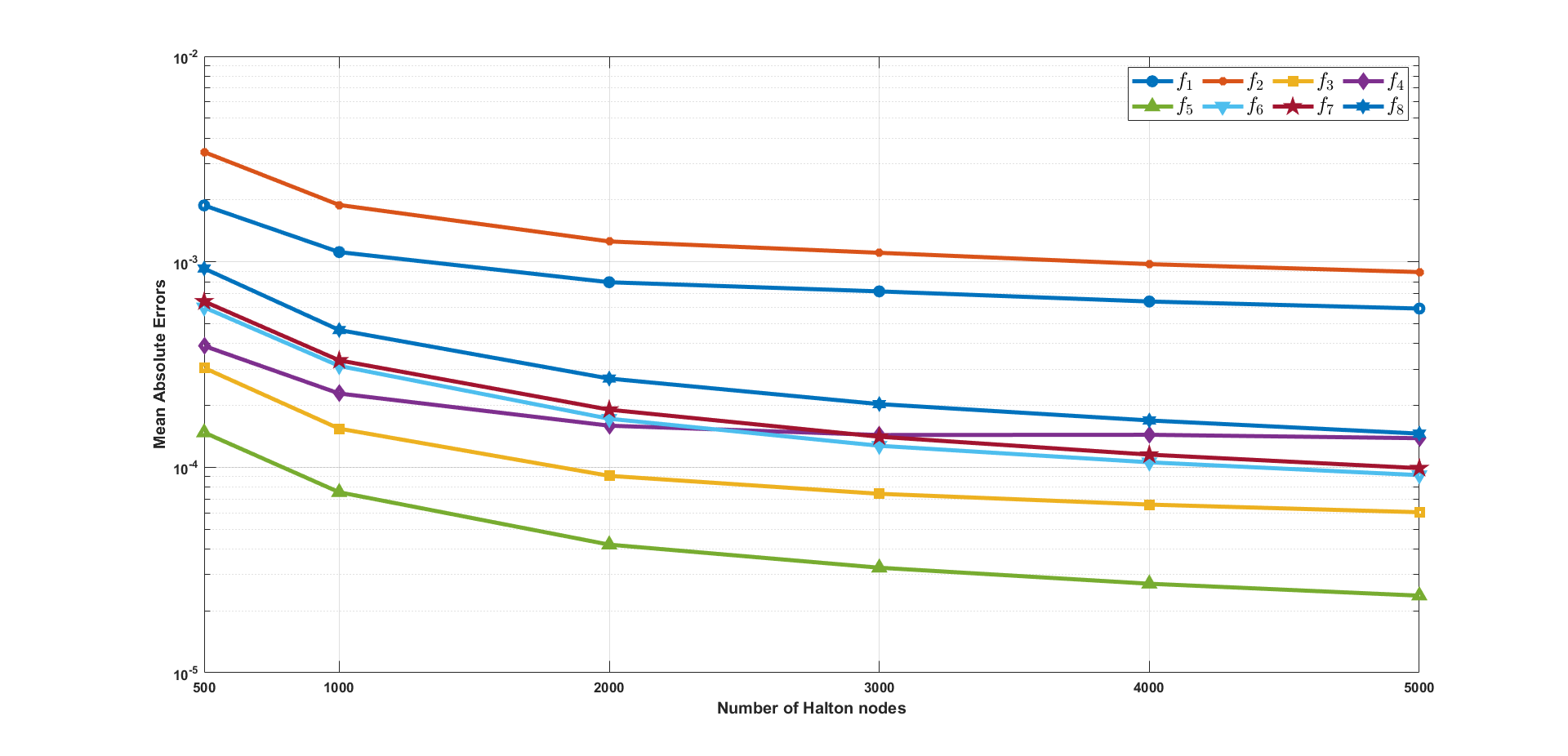
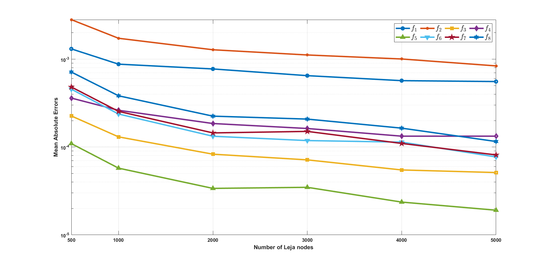
We also plot the mean absolute errors (), considering , nodes (see Halton case in Figure 1 and Leja case in Figure 2) to evaluate the operator on spiral points.
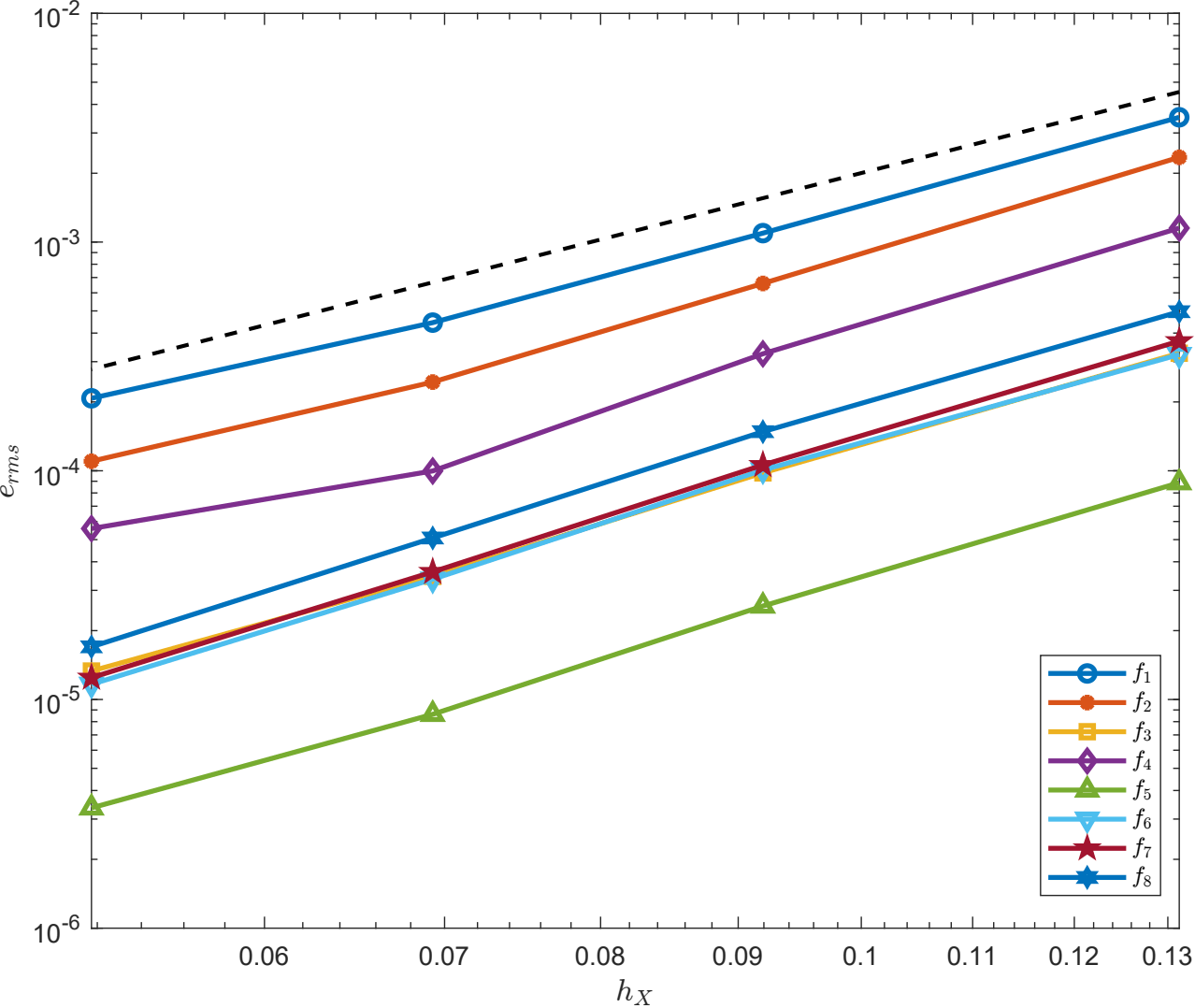
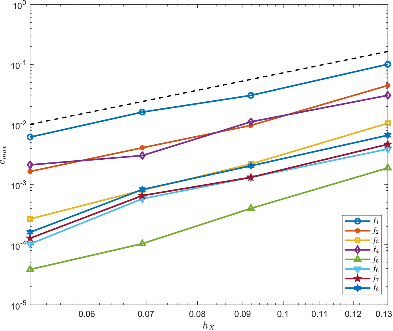
We now present, in Figure 3, the log-log plots of the root mean square error () and the maximum error () versus the fill distance , obtained using Halton nodes and all eight test functions, evaluated at spiral points. For reference, the black dashed line indicates the theoretical cubic trend.
Next, we compare the operator , introduced in (11) with several operators from the literature: the classical spherical Shepard operator given in (1), the modified variant defined in (4), the Shepard-Bernoulli operator introduced in [6], and the augmented Shepard operators and , constructed using the thin-plate spline and inverse multiquadric spherical radial basis functions (SBFs) [5].
The Shepard-Bernoulli operator of order is defined in Eq. (4.4) in [6]. Here, we consider the case , since higher orders also require the partial derivatives of the function. Consider the Delaunay triangulation of the sphere and the number of triangles that form the triangulation. We let denote a triangle from the triangulation, with vertices , such that each node is a vertex of at least one triangle, i.e.,
Consider also for a point , its barycentric coordinates relative to , which are defined as
with representing the signed area of the triangle with vertices .
The Shepard-Bernoulli operator of order is given as
| (19) |
with
and
The augmented spherical radial basis function operators and are defined in Eq. (2.10) and Eq. (2.12) in [5], respectively, as
| (20) |
Here, the augmented local zonal basis function is of the following particular form
for and with being defined in the thin-plate spline case as and in the inverse multiquadric case as .
The index set contains the nearest neighbors of the node and the coefficients are obtained by imposing general interpolation conditions and constraints from the radial basis function theory. For more details, one can consult [5] and the references therein.
We considered spiral evaluation points and two sets of nodes: Halton nodes and Leja nodes. The maximum absolute errors (), mean absolute errors (), root mean square errors (), and CPU times are presented in Table 5 for the Halton-nodes case and in Table 6 for the Leja-nodes case. We can observe that the proposed operator outperforms the classical and modified variants of the Shepard operator, as well as the variants based on spherical radial basis functions, in terms of approximation accuracy. It is also faster than both SBF-augmented variants. Compared with the Bernoulli variant, the errors of the two operators are, in most cases, of the same order, while the operator introduced in this paper requires less CPU time. Nonetheless, the Bernoulli variant is constructed somewhat differently from the least squares spherical Shepard operator, since it relies on the Delaunay triangulation of the sphere and different basis functions.
| CPU(s) | |||||||
|---|---|---|---|---|---|---|---|
| CPU(s) | |||||||
| CPU(s) | |||||||
| CPU(s) | |||||||
| CPU(s) | |||||||
| CPU(s) | |||||||
| CPU(s) | |||||||
| CPU(s) |
| CPU(s) | |||||||
|---|---|---|---|---|---|---|---|
| CPU(s) | |||||||
| CPU(s) | |||||||
| CPU(s) | |||||||
| CPU(s) | |||||||
| CPU(s) | |||||||
| CPU(s) | |||||||
| CPU(s) |
4 Applications to real-data problems
To illustrate the practical benefits of the method introduced in this paper, we apply the proposed operator to reconstruct meteorological data. We use a dataset downloaded from https://www.kaggle.com/datasets/jakubkrasuski/global-weather-data-conditions-for-209579-cities, which contains current weather conditions for cities around the world (the dataset used is from February 2025). As noted by the authors, the dataset includes numerous measurements of meteorological variables such as temperature, pressure, humidity, wind characteristics, cloudiness, and precipitation. We randomly selected sample points from the dataset as nodes and reconstructed the corresponding values at evaluation points. Although the nodes were randomly selected, we ensured that they remained sufficiently uniformly distributed such that no geographic regions were left unsampled. However, in cases where certain evaluation points were located far away from all other nodes (i.e., no neighboring node lay within a radius of ), we treated them as outliers and excluded them from the error analysis, since an accurate reconstruction is not possible in the absence of nearby supporting data. The percentage of discarded points was very small (at most for nodes and at most for nodes), and it did not meaningfully influence the results. Below, we present different practical applications of the Shepard operator introduced in (11). The operator is constructed using local quadratic polynomials , as described in (9), and various choices for the number of nodes and evaluation points. In each case, we compute the mean absolute error () and the root mean square error ().
4.1 Pressure approximation
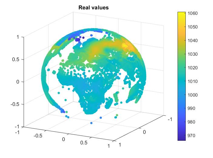
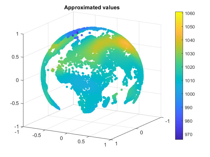
We first consider the problem of reconstructing atmospheric pressure values in different zones on Earth. The dataset contains values between and . The errors are displayed in Table 7 and a graphical representation of the actual and approximated values in the case of nodes and evaluation points is presented in Figure 4. The relative error in all the cases is .
| () | ||||||
|---|---|---|---|---|---|---|
| () | ||||||
4.2 Temperature approximation
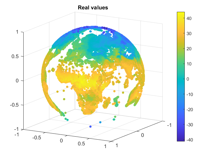
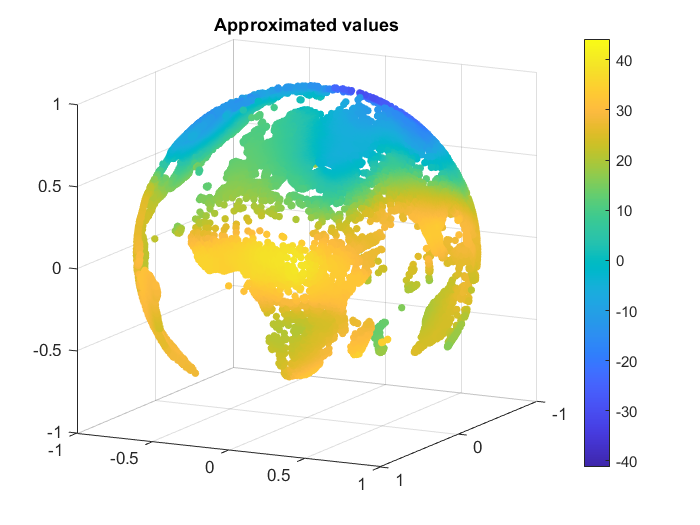
We next consider the problem of reconstructing temperature values on the globe. The minimum temperature in the dataset is and the maximum temperature is . The errors are displayed in Table 8, and a graphical representation of the actual and approximated values in the case of nodes and evaluation points is presented in Figure 5. The relative error in all the cases is .
| () | ||||||
|---|---|---|---|---|---|---|
| () | ||||||
4.3 Wind speed approximation
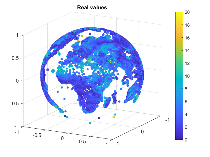
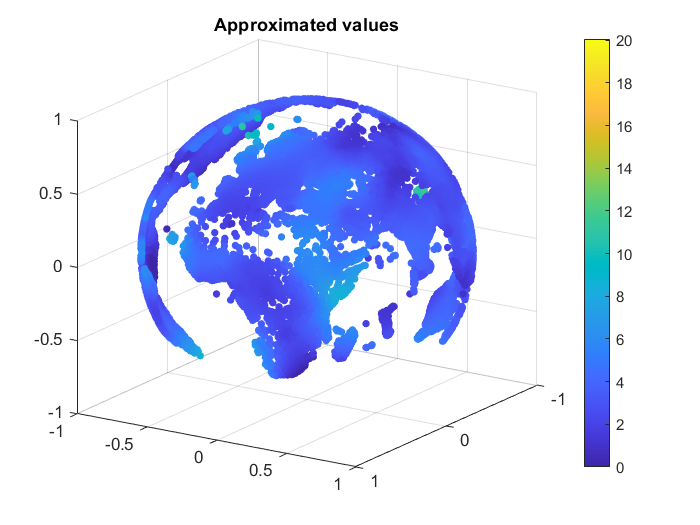
We now investigate the problem of wind speed approximation. The values are given in , with a range between and . Table 9 displays the approximation errors and Figure 6 shows the graphical representation of the real and approximated values.
| () | ||||||
|---|---|---|---|---|---|---|
| () | ||||||
4.4 Rainfall approximation
The last practical application of the operator introduced in (11) that we study in this paper is the approximation of rainfall amounts (precipitation) in mm measured in an hour. We considered only the non-zero values, which left us with values between and . Table 10 presents the approximation errors for different choices of the number of nodes () and evaluation points ().
| () | ||||||
|---|---|---|---|---|---|---|
| () | ||||||
Finally, we study the behavior of the operators presented above in reconstructing the data associated with the phenomena discussed in this section. The operators investigated are the following: the Shepard-type operator proposed in this paper and defined in (11), the classical Shepard operator given in (1), the modified variant defined in (4), the Shepard-Bernoulli operator of order , , defined in (19), and the variant combined with the thin-plate spline spherical radial basis function, , from (20). We consider evaluation points and use sets of and nodes. The corresponding results are presented in Table 11 and Table 12, respectively.
We can observe that, for wind speed and precipitation, the best approximation results are given by the simple operators, classical and modified . For pressure, the Shepard-Bernoulli operator achieves the lowest errors among all the operators considered. For temperature, the results are mixed, but achieves the smallest root mean square error in both tables. Overall, and are comparable, with performing better for wind speed and, in most cases, for precipitation, while performs better for pressure and, with respect to the mean absolute error, for temperature. However, has an advantage in terms of computational time. The proposed operator outperforms in the majority of the cases considered. Besides requiring less computational time than the combined operators and in these experiments, the proposed operator has an advantage over higher-order Shepard-Bernoulli operators: its local polynomials, even when a higher polynomial degree is used, can be constructed from observed function values alone, without requiring partial derivatives, which are generally unavailable in meteorological and other observational datasets. Nevertheless, the numerical results in the preceding two sections show that the dataset influences the outcome, as is known to happen in this kind of problem.
| Pressure () | ||||||
|---|---|---|---|---|---|---|
| CPU(s) | ||||||
| Temperature () | ||||||
| CPU(s) | ||||||
| Wind speed () | ||||||
| CPU(s) | ||||||
| Precipitation () | ||||||
| CPU(s) |
| Pressure () | ||||||
|---|---|---|---|---|---|---|
| CPU(s) | ||||||
| Temperature () | ||||||
| CPU(s) | ||||||
| Wind speed () | ||||||
| CPU(s) | ||||||
| Precipitation () | ||||||
| CPU(s) |
References
- [1] Allasia, G., Cavoretto, R., De Rossi, A.: Hermite-Birkhoff interpolation on scattered data on the sphere and other manifolds. Appl. Math. Comput. 318, 35–50 (2018)
- [2] Bos, L., De Marchi, S., Sommariva, A., Vianello, M.: Computing multivariate Fekete and Leja points by numerical linear algebra. SIAM J. Numer. Anal. 48(5), 1984–1999 (2010)
- [3] Bos, L., De Marchi, S., Sommariva, A., Vianello, M.: On multivariate Newton interpolation at discrete Leja points. Dolomites Res. Notes Approx. 4, 15–20 (2010)
- [4] Calvi, J.P., Levenberg, N.: Uniform approximation by discrete least squares polynomials, J. Approx. Theory 152, 82–100 (2008)
- [5] Cătinaş, T., Malina, A.: Spherical interpolation of scattered data using least squares thin-plate spline and inverse multiquadric functions. Numer. Algor. 97, 1397–1414 (2024)
- [6] Cătinaş, T., Malina, A.: Spherical Shepard-Bernoulli operator. J. Appl. Math. Comput. 71, 1267–1283 (2025)
- [7] Cavoretto, R., De Rossi, A.: Fast and accurate interpolation of large scattered data sets on the sphere. J. Comput. Appl. Math. 234, 1505–1521 (2010)
- [8] Cavoretto, R., De Rossi, A.: Numerical comparison of different weights in Shepard’s interpolants on the sphere. Appl. Math. Sci. 4, 3425–3435 (2010)
- [9] Cavoretto, R., De Rossi, A.: Spherical interpolation using the partition of unity method: An efficient and flexible algorithm. Appl. Math. Lett. 25, 1251–1256 (2012)
- [10] Cavoretto, R., De Rossi, A.: Achieving accuracy and efficiency in spherical modelling of real data. Math. Methods Appl. Sci. 37, 1449–1459 (2014)
- [11] Cheney, E.W., Light, W.A.: A Course in Approximation Theory, vol. 101. American Mathematical Soc. (2009)
- [12] Davydov, O., Schumaker, L.L.: Scattered data fitting on surfaces using projected Powell-Sabin splines. In: Martin, R., Sabin, M., Winkler, J. (eds) Mathematics of Surfaces XII. Mathematics of Surfaces 2007. Lecture Notes in Computer Science, vol 4647. Springer, Berlin, Heidelberg (2007)
- [13] De Rossi, A.: Spherical interpolation of large scattered data sets using zonal basis functions. In: Daehlen, M., Morken, K., Schumaker, L. (eds.) Mathematical Methods for Curves and Surfaces Trømso 2004, Nashboro Press, 125–134 (2005)
- [14] Farwig, R.: Rate of convergence of Shepard’s global interpolation formula. Math. Comp. 46, 577–590 (1986)
- [15] Franke, R.: Scattered data interpolation: tests of some methods. Math. Comp. 38, 181–200 (1982)
- [16] Franke, R., Nielson, G.: Smooth interpolation of large sets of scattered data. Int. J. Numer. Meths. Engrg. 15, 1691–1704 (1980)
- [17] Le Gia, Q., Sloan, I., Wendland, H.: Multiscale analysis in Sobolev spaces on the sphere. SIAM J. Numer. Anal. 48, 2065–2090 (2010)
- [18] Little, F.: Convex combination surfaces. In: Barnhill, R.E., Boehm, W. (eds) Surfaces in Computer Aided Geometric Design, Amsterdam: North-Holland, 99–107 (1983)
- [19] Nielson, G., Ramaraj, R.: Interpolation over a sphere based upon a minimum norm network. Comput. Aided Geom. Design 4, 41–57 (1987)
- [20] Renka, R.J.: Interpolation of data on the surface of a sphere. ACM Trans. Math. Software 10, 417–436 (1984)
- [21] Renka, R.J., Cline, A.K.: A triangle-based interpolation method. Rocky Mountain J. Math. 14, 223–237 (1984)
- [22] Renka, R.J.: Multivariate interpolation of large sets of scattered data. ACM Trans. Math. Software 14, 139–148 (1988)
- [23] Shepard, D.: A two dimensional interpolation function for irregularly spaced data. In: Proceedings of the 1968 23rd ACM National Conference, 517–523. ACM (1968)
- [24] Wendland, H.: Scattered Data Approximation. Cambridge University Press (2004)
- [25] Wong, T.T., Luk, W.S., Heng, P.A.: Sampling with Hammersley and Halton Points. J. Graph. Tools, 2(2), 9–24 (1997)
- [26] Zerroudi, B., Tayeq, H., El Harrak, A.: Effective interpolation of scattered data on a sphere through a Shepard-like method. Math. Model. Comput. 10(4), 1174–1186 (2023)
- [27] Zerroudi, B., Tayeq, H., El Harrak, A.: Scattered data interpolation on the 2-dimensional surface through Shepard-like technique. Math. Model. Comput. 11(1), 277–289 (2024)
- [28] Zuppa, C.: Error estimates for moving least square approximations. Bull. Braz. Math. Soc. 34(2), 231–249 (2003)
[1] Allasia, G., Cavoretto, R., De Rossi, A.: Hermite-Birkhoff interpolation on scattered data on the sphere and other manifolds. Appl. Math. Comput. 318, 35–50 (2018)
[2] Bos, L., De Marchi, S., Sommariva, A., Vianello, M.: Computing multivariate Fekete and Leja points by numerical linear algebra. SIAM J. Numer. Anal. 48(5), 1984–1999 (2010)
[3] Bos, L., De Marchi, S., Sommariva, A., Vianello, M.: On multivariate Newton interpolation at discrete Leja points. Dolomites Res. Notes Approx. 4, 15–20 (2010)
[4] Calvi, J.P., Levenberg, N.: Uniform approximation by discrete least squares polynomials, J. Approx. Theory 152, 82–100 (2008)
[5] Cătinaș, T., Malina, A.: Spherical interpolation of scattered data using least squares thin-plate spline and inverse multiquadric functions. Numer. Algor. 97, 1397–1414 (2024)
[6] Cătinaș, T., Malina, A.: Spherical Shepard-Bernoulli operator. J. Appl. Math. Comput. 71, 1267–1283 (2025)
[7] Cavoretto, R., De Rossi, A.: Fast and accurate interpolation of large scattered data sets on the sphere. J. Comput. Appl. Math. 234, 1505–1521 (2010)
[8] Cavoretto, R., De Rossi, A.: Numerical comparison of different weights in Shepard’s interpolants on the sphere. Appl. Math. Sci. 4, 3425–3435 (2010)
[9] Cavoretto, R., De Rossi, A.: Spherical interpolation using the partition of unity method: An efficient and flexible algorithm. Appl. Math. Lett. 25, 1251–1256 (2012)
[10] Cavoretto, R., De Rossi, A.: Achieving accuracy and efficiency in spherical modelling of real data. Math. Methods Appl. Sci. 37, 1449–1459 (2014)
[11] Cheney, E.W., Light, W.A.: A Course in Approximation Theory, vol. 101. American Mathematical Soc. (2009)
[12] Davydov, O., Schumaker, L.L.: Scattered data fitting on surfaces using projected Powell-Sabin splines. In: Martin, R., Sabin, M., Winkler, J. (eds) Mathematics of Surfaces XII. Mathematics of Surfaces 2007. Lecture Notes in Computer Science, vol 4647. Springer, Berlin, Heidelberg (2007)
[13] De Rossi, A.: Spherical interpolation of large scattered data sets using zonal basis functions. In: Daehlen, M., Morken, K., Schumaker, L. (eds.) Mathematical Methods for Curves and Surfaces Trømso 2004, Nashboro Press, 125–134 (2005)
[14] Farwig, R.: Rate of convergence of Shepard’s global interpolation formula. Math. Comp. 46, 577–590 (1986)
[15] Franke, R.: Scattered data interpolation: tests of some methods. Math. Comp. 38, 181–200 (1982)
[16] Franke, R., Nielson, G.: Smooth interpolation of large sets of scattered data. Int. J. Numer. Meths. Engrg. 15, 1691–1704 (1980)
[17] Le Gia, Q., Sloan, I., Wendland, H.: Multiscale analysis in Sobolev spaces on the sphere. SIAM J. Numer. Anal. 48, 2065–2090 (2010)
[18] Little, F.: Convex combination surfaces. In: Barnhill, R.E., Boehm, W. (eds) Surfaces in Computer Aided Geometric Design, Amsterdam: North-Holland, 99–107 (1983)
[19] Nielson, G., Ramaraj, R.: Interpolation over a sphere based upon a minimum norm network. Comput. Aided Geom. Design 4, 41–57 (1987)
[20] Renka, R.J.: Interpolation of data on the surface of a sphere. ACM Trans. Math. Software 10, 417–436 (1984)
[21] Renka, R.J., Cline, A.K.: A triangle-based C1 interpolation method. Rocky Mountain J. Math. 14, 223–237 (1984)
[22] Renka, R.J.: Multivariate interpolation of large sets of scattered data. ACM Trans. Math. Software 14, 139–148 (1988)
[23] Shepard, D.: A two dimensional interpolation function for irregularly spaced data. In: Proceedings of the 1968 23rd ACM National Conference, 517–523. ACM (1968)
[24] Wendland, H.: Scattered Data Approximation. Cambridge University Press (2004)
[25] Wong, T.T., Luk, W.S., Heng, P.A.: Sampling with Hammersley and Halton Points. J. Graph. Tools, 2(2), 9–24 (1997)
[26] Zerroudi, B., Tayeq, H., El Harrak, A.: Effective interpolation of scattered data on a sphere through a Shepard-like method. Math. Model. Comput. 10(4), 1174–1186 (2023)
[27] Zerroudi, B., Tayeq, H., El Harrak, A.: Scattered data interpolation on the 2-dimensional surface through Shepard-like technique. Math. Model. Comput. 11(1), 277–289 (2024)
[28] Zuppa, C.: Error estimates for moving least square approximations. Bull. Braz. Math. Soc. 34(2), 231–249 (2003)