Abstract
We are concerned with stable spectral collocation solutions to non-periodic Benjamin Bona Mahony (BBM), modified BBM and Benjamin Bona Mahony-Burgers (BBM-B) initial value problems on the real axis. The spectral collocation is based alternatively on the scaled Hermite and sinc functions. In order to march in time we use several one step and linear multistep finite difference schemes such that the method of lines (MoL) involved is stable in sense of Lax. The method based on Hermite functions ensures the correct behavior of the solutions at large spatial distances and in long time periods. In order to prove the stability we use the pseudospectra of the linearized spatial discretization operators. The extent at which the energy integral of BBM model is conserved over time is analyzed for Hermite collocation along with various finite difference schemes. This analysis has been fairly useful in optimizing the scaling parameter. The effectiveness of our approach has been confirmed by some numerical experiments.
Authors
Călin-Ioan Gheorghiu
(Tiberiu Popoviciu Institute of Numerical Analysis, Romanian Academy)
Keywords
References
See the expanding block below.
Paper coordinates
C.I. Gheorghiu, Stable spectral collocation solutions to a class of Benjamin Bona Mahony initial value problems. Appl. Math. Comp., 273 (2016) 1090-1099
doi: 10.1016/j.amc.2015.10.078
About this paper
Print ISSN
0096-3003
Online ISSN
Google Scholar Profile
google scholar link
Paper (preprint) in HTML form
Stable Spectral Collocation Solutions to a Class of Benjamin Bona Mahony Initial Value Problems
Abstract
We are concerned with stable spectral collocation solutions to non-periodic Benjamin Bona Mahony (BBM), modified BBM and Benjamin Bona Mahony-Burgers (BBM-B) initial value problems on the real axis. The spectral collocation is based alternatively on the scaled Hermite and sinc functions. In order to march in time we use several one step and linear multistep finite difference schemes such that the method of lines (MoL) involved is stable in sense of Lax. The method based on Hermite functions ensures the correct behavior of the solutions at large spatial distances and in long time periods. In order to prove the stability we use the pseudospectra of the linearized spatial discretization operators. The extent at which the energy integral of BBM model is conserved over time is analyzed for Hermite collocation along with various finite difference schemes. This analysis has been fairly useful in optimizing the scaling parameter. The effectiveness of our approach has been confirmed by some numerical experiments.
Key words: regularized long wave equation; scaled Hermite collocation; method of lines; Lax stability; energy conservation;
1 Introduction
The purpose of this paper is the analysis and practical development of the method of lines (MoL for short) based on spectral collocation and various finite difference schemes as an efficient tool to solve the Cauchy’s problem attached to a class of Benjamin Bona Mahony (BBM for short) equations. The most representative equation reads
| (1) |
whose solution is considered in a class of non-periodic functions defined on and
For and the equation (1) is called Benjamin Bona Mahony or the regularized long-wave equation. It has been introduced by the above mentioned mathematicians in the early ’70 (see [1]) as a counterpart of the well known Korteweg-de Vries (KdV) equation
| (2) |
When and the equation (1) will be called modified BBM equation and for and we will refer at (1) as to the Benjamin Bona Mahony-Burgers (BBM-B for short) one.
In (1), as well as in the formulation of (2), represents the vertical displacement of the surface of the liquid (ideal fluid) from its equilibrium position, is the time and is the horizontal coordinate which increases in the direction of waves propagation. Both equations are in dimensionless form with the length scale taken to be the unperturbed depth of the liquid and time scale be is the gravity constant.
The authors of [1] compare in various ways their regularized long-wave equation with KdV and argue that the latter has some shortcomings which makes that an unsuitable posed model for long waves (see also [2]). We do not want to get involved into the details of this debate but we observe that the BBM model has received less attention from numerical point of view than the KdV one.
One of the purposes of this work is to try to fill this gap providing reasonable numerical wave solutions without an artificial (empirical) truncation of the domain or periodicity assumptions.
For a model equation for long waves, periodic solutions have been obtained in the early era of modern computational mathematics by Galerkin method in [19]. On a finite interval, an initial-(Dirichlet) boundary value problem attached to BBM has been solved by Galerkin method in [13] and by a Crank-Nicolson-type finite difference method in [14].
A kind of Hermite spectral method has been used in [11] in order to solve KdV, a modified KdV and the nonlinear Schroedinger equations. The so called KdV solitons of Boyd have been detected this way. However, in [3] it is observed that the Hermite functions are the exact eigenfunctions of quantum mechanics harmonic oscillator and are the asymptotic eigenfunctions for Mathieu’s equation, the prolate spheroidal wave equation, the associated Legendre equation, and Laplace’s Tidal equation. This close connection with the physics makes Hermite functions a fairly natural choice of basis functions for various fields of science and engineering.
In a recent laborious study [4] the authors extend the framework of the finite volume methods to dispersive water wave models, in particular to Boussinesq type systems.
In this context, we focus in this paper on the mathematical aspects of the spectral collocation methods, mainly based on Hermite functions, as an efficient tool in modeling the dispersion of long waves. Along with some implicit time schemes, the involved MoL, accurately conserves a quadratic invariant of the flow and resolves correctly the asymptotic behavior of the solutions at large distances.
Specifically, we will be concerned in the first instance with the Cauchy’s problem
| (3) |
where the initial data satisfies the conditions
-
1.
-
2.
Then the problem (3) has a solution At any the solution and its derivative along with all their derivatives with respect to are asymptotically null i.e.,
| (4) |
Additionally, is conserved over time, i.e., where
| (5) |
With respect to the first condition on the initial data the authors of [1] observe that in fact an element of and its first derivative , both converge to at The functional introduced with (5) is called energy integral although it is not necessarily identifiable with the energy in the original physical problems.
In order to describe the smoothness of solution the authors quoted above introduce the space of continuous functions on equipped with the maximum norm and its subspace of functions such that for and equipped with the subsequent norm. The space is the usual Sobolev space of functions over with generalized first derivative which is also function.
We will heavily rely on this analytical result. Moreover this fundamental result on the existence, uniqueness and asymptotic behavior of non-periodic solutions to (3) has suggested a collocation approach of the spatial dependence using Hermite (HC for short) as well as sinc functions (SC for short). In this context fairly accurate differentiation matrices corresponding to these functions are needed. They are available in [5] and in the seminal paper [20].
Actually, the HC method is used in the same spirit in which the Laguerre collocation (LC) has been successfully used in our previous papers [6] and [7]. With LC, as well as with HC, we avoid the frequently used empirical treatment of boundary value problems defined on the infinite domains based on the arbitrary truncation of the domain.
In order to march in time we have used gradually one step explicit methods such as Runge-Kutta (RK) methods of orders , and and linear multistep methods such as Adams-Bashforth (AB for short), Adams-Moulton (AM for short) and leap frog schemes. The regions of stability of all these finite differences formulas along with the spectral properties of Hermite and sinc differentiation matrices of moderate orders , i.e., have assured the numerical stability of MoL. The necessary and sufficient conditions of Lax-stability formulated in [9] and [16] have been rigorously observed.
A particular attention is paid to the conservation of energy integral over time. The time marching schemes as well as the spatial collocation schemes are evaluated with respect to this aspect. More precisely, the scaling parameter involved in the HC has been adjusted in order to optimize the conservation of this invariant. Meantime this scaling factor has also been chosen in order to enlarge the spatial interval of integration. This way we have succeeded in capturing the evolution of the initial front on fairly long time intervals. Some differences between HC and SC methods have been noticed in this context.
The paper is organized as follows. In Section 2 we solve the BBM problem as well as a modified BBM problem by Hermite and sinc spectral collocation methods along with Runge-Kutta method of order 4. Then we show the stability of this MoL as well as of the MoL based on the other finite difference schemes mentioned above. The last subsection is devoted to the conservation of the energy invariant. As we do not have a general rule to establish a correct value of the scaling parameter, this conservation process is in fact the key in its optimal choosing. The Section 3 parallelizes, up to some point, the previous one corresponding to the BBM-B problem. Actually, in both sections the normality of the differentiation matrices as well as of the linearized spatial discretization operators have been quantified using a scalar measure, i.e., the Henrici’s number and their pseudospectra. Then we make use of the Trefethen’s rule of thumb, which states: a MoL is stable if the eigenvalues of the (linearized) spatial discretization operator, scaled by , lie in the stability region of the time-discretization operator (see [18], p. 103). Fortunately, the matrices involved in the problems at hand are not far from normal and thus this rule makes accurate predictions. In some way the rule can be thought of as an analogue of the well known CFL condition. Section 4 reviews our main results.
2 The MoL for BBM initial value problem
In order to solve problem (3) we rewrite the differential equation in the following convenient form
| (6) |
2.1 The HC method
The interpolant of a map reads
| (7) |
where
is the Hermite polynomial of degree defined by the three term recurrence formula
with
The nodes are the roots of indexed in the ascending order. The Hermite differentiation matrices will be denoted by for They are provided along with the above roots by the MATLAB code herdif from [20]. Actually, we work with the scaled roots and consequently the differentiation matrices correspond to these scaled nodes. The Hermite differentiation process is exact for functions of the form
where is a polynomial of degree or less, assuming exact arithmetic. The scaling factor will be exploited in our numerical experiments in some respects.
However, the rate of convergence theory for Hermite functions is now well established for a fixed ( independent) scale factor (see [3], § 17.4 ”Hermite functions”). This rate depends not only on the location of singularities, as it is true for all spectral expansions, but also upon the rate at which a given function decays as
The MoL applied to problem (3) along with HC means to approximate the solution of this problem (using the form (6)) with
| (8) |
Thus, the conditions (4) are satisfied and the problem is transformed into the Cauchy’s problem for the following system of ODE
| (9) |
where is the unit matrix of order , and
The ”mass” matrix is nonsingular and independent of and , so this system is fairly amenable to be solved by some ode built-in functions of MATLAB. The period character in the r. h. s. of the semidiscretized problem (9) signifies the array power of vector
In order to assert the Lax stability of this MoL we have to analyze the linearized spatial discretization operator attached to (9). This is in fact the matrix
| (10) |
The Frobenius norm conditioning and the Henrici’s number of the matrices and are displayed in Table 1.
Remember that for a square matrix the Henrici’s number is defined by
where stands for the Frobenius norm of and is the conjugate transpose of Thus a matrix is normal iff and ( see for instance our contribution [8]).
The sinc differentiation matrices are symmetric or skew-symmetric for even respectively odd values of the cut off parameter The Hermite differentiation matrices look worse from this point of view but are still closed to the normality.
| Matrices | ||||||
|---|---|---|---|---|---|---|
| Method | Hermite | sinc | Hermite | sinc | Hermite | sinc |
| Conditioning | 9.44e+01 | 6.29e+01 | 6.35e+03 | 4.09e+03 | 4.67e+01 | 7.78e+02 |
| Henrici | 1.39e-01 | 0 | 2.94e-02 | 0 | 2.27e-02 | 8.69e-01 |
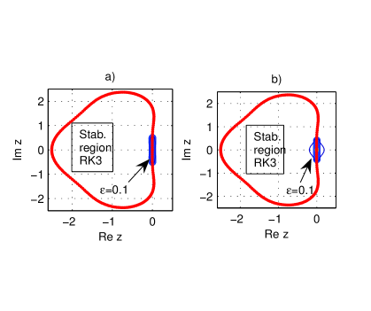
The pseudospectra of are depicted in Fig. 1 for two values of scaling parameter. The eigenvalues of lie on the right hand side boundary of the stability region of RK3. For the operator is almost normal. This statement is based on its pseudospectrum from Fig. 1 a) and its Henrici’s number (the bold value in Tab. 1). Even for a larger value of scaling factor, i.e. half of the largest contour of the pseudospectrum, i.e., corresponding to is situated inside the stability region and the other half lies within a distance of order for ”small” and approaching
This is the first reason in working with
In accordance with the above quoted Trefethen’s rule of thumb, this assures the numerical stability of MoL based on RK3 and HC.
A similar and even better situation occurs when instead of RK3 a higher order method, namely RK4 is used. Fairly clear and explicit figures concerning the stability regions corresponding to various RK, AB and AM methods are available for instance in [15] p.215.
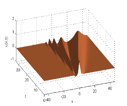
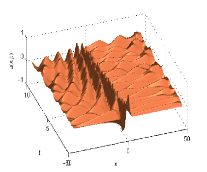
The solution to BBM (3) when is depicted in Fig. 2. The scaling factor has been chosen equal to In this way we enlarge the span of evolution of initial data. A second reason for a scaling factor less than unity.
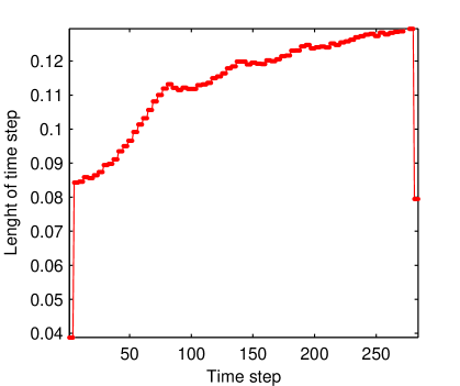
In order to implement the Runge-Kutta method we have used the MATLAB built-in function ode45. In spite of the large integration time no floating point overflow has been observed. The whole computation involves some seconds and 284 time steps on our HP xw8400 workstation with clock speed of 3.2 Ghz.
The evolution of the time steps length is illustrated in Fig. 3.
From physical point of view, it appears from Fig. 2 that, as time proceeds, new solitary waves have emerged from the initial profile. More exactly, the first wave emerged immediately from the initial one and the fourth one still had considerable evolution to undergo before it could reasonably be said to have established its asymptotic form. This development over time is perfectly identical with that described in [2] p. 265. In this paper the initial front has the form
It is also fairly important to mention that the numerical value of the ”energy” functional oscillates with largest errors of order during the integration time (see Section 2.3). For the above initial front we have the estimation
We have also carried out numerical experiments with the following initial fronts: and All these functions are continuous ones but not continuously differentiable. They, along with their first derivatives, approach as Thus they do not satisfy the first requirement of smoothness for the initial data imposed in the existence theorem quoted in Introduction. In spite of this lack of smoothness, for each front above, a solution to problem (9) and consequently to the problem (3) has been produced. As natural, all these solutions inherit the defect of smoothness of their initial fronts.
A MATLAB animation can be easily set up in order to show the breaking up of the initial front into subsequent solitary waves.
2.2 The SC method
In order to apply this method we use equidistant nodes with spacing symmetric with respect the origin, namely
The interpolant for a real valued function reads
where the sinc or ”Whittaker cardinal” functions are
Like the Hermite method, the sinc method contains a free parameter, namely the step size The typical estimate for is for some constant independent of Unfortunately the information provided in [17] for this constant is rather poor. In this work the author analyzes the application of various methods (Galerkin and collocation) based on sinc functions in solving a large variety of equations. It is interesting to remark that he solves differential boundary value problems only on finite intervals but otherwise with endpoint singularities.
The sinc expansion is the easiest of all pseudospectral methods to program and to understand (see [3], § ”Whittaker Cardinal or ”Sinc” Functions”). Unfortunately, its success is assured only for the so called band-limited functions. Another weakness, shared with the Hermite functions, is that the sinc series is useful only when it approximates a function which decays exponentially as Unlike the Hermite functions, they do not provide the exact solution to any classical eigenvalue problem.
The sinc differentiation matrices are available in [20]. The linearized spatial discretization operator attached to (9) in this case is defined by
| (11) |
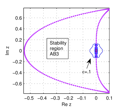
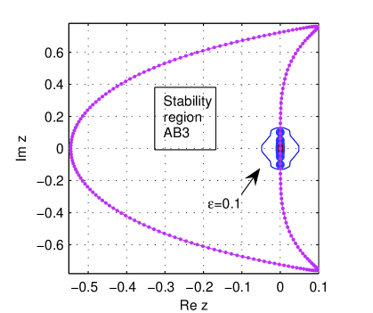
From the last two columns of Table 1 it is apparent that is better conditioned and more normal than The pseudospectrum for is depicted in Fig. 4. In order to advocate the versatility of MoL for BBM type equations we overlapped this pseudospectrum with the stability region AB of order 3.
2.3 Conservation of the energy integral
It is fairly important to observe to what extent various finite difference schemes along with the scaled HC method generate a MoL which conserves the ”energy” over time, i.e., the integral (5) is indeed an invariant of the physical system.
In Fig. 5 a) for a scaling factor and in Fig. 5 b) for the outcomes provided by MATLAB codes ode45, ode23 and ode15s in solving (9) are compared. We mention that the codes ode45, ode23 implement respectively RK4 and RK2 schemes and ode15s implements a variable order solver based on the numerical differentiation formulas (NDF).
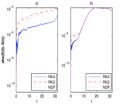
The RK4 used along with performs the best. Actually, this is the main reason we have worked with . In our numerical experiments this value of has been proved to be the most suitable.
We have to emphasize that these errors in conserving the energy, as well as the solution itself strongly depend on the scaling factor. All our numerical experiments revealed the necessity for such a factor to be less than unity. In this way for the outmost scaled Hermite roots we have the estimation
Thus, with we extend the span for the wave propagation and we can follow the wave for larger time intervals.
It is also worth mentioning that our numerical estimations satisfy the inequality (see also Fig. 2)
| (12) |
which is in perfect accordance with the analytical results reported in [1]. The estimation is independent of and for and .
In order to compute the integral we have used the Gauss-Hermite quadrature rule (see for instance [12], § 3.5 ”Quadrature: Gauss–Hermite Formula”). The term in the integrand was estimated using the first order Hermite differentiation matrix .
Unfortunately, for sinc collocation, due to the distribution of the collocation nodes such strategy is rather impossible. This is the main explanation for the fact that in spite of the well defined MoL based on these functions our numerical experiments restrict to the Hermite case. Roughly speaking, it seems that the evolution of some large waves can not be detected using band-limited functions.
3 The MoL for the modified BBM initial value problem
The linearizations of this problem look identical with (10) and (11) respectively. An usual computation (multiplication with and integration by parts) shows that must be conserved over time independent of in the BBM equation. For the situation is illustrated in Fig. 6 and comparing with Fig. 5 it is clear that the conservation process is at least as accurate as that in BBM problem.
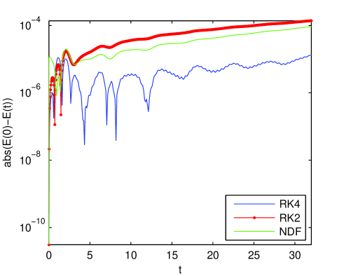
The solution of the modified BBM problem with this value of looks fairly similar with that depicted in Fig. 2, i.e., certain classes of initial data evolve into a sequence of solitary waves followed by a dispersive wave train. Thus we skip such a picture. In Fig. 6 we use the same notations as in Fig. 5.
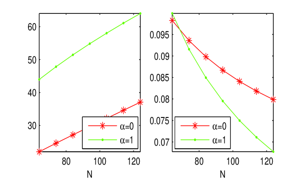
One important remark about the linearized operators is well suited at this moment. The conditioning of is increasing with the parameter and the order of approximation (see the left panel in Fig. 7). This is a fairly intuitive aspect. With respect to the normality of this operator the situation is reversed, namely the Henrici number of slightly decreases when as well as the order of approximation increases for a fixed value of the scaling parameter . The latter aspect could partially explain the success of the HC method.
4 The MoL for BBM-B initial value problem
It is again convenient to write the (1) equation in the following form
| (14) |
The MoL based on the HC for to the initial value problem attached to the equation (14) reads
| (15) |
The corresponding linearized spatial discretization operator for (15) is now
The spectral properties of and depending on the diffusion parameter are summarized in Table 2. At a first glance it is clear that for decreasing the properties of the Hermite operator are better than those of the sinc one.
| Method | Hermite | sinc | Hermite | sinc |
| Conditioning | 1.64e+01 | 1.20e+00 | 4.64e+01 | 9.29e+01 |
| Henrici | 9.54e-02 | 2.79e-02 | 2.27e-02 | 8.29e-01 |
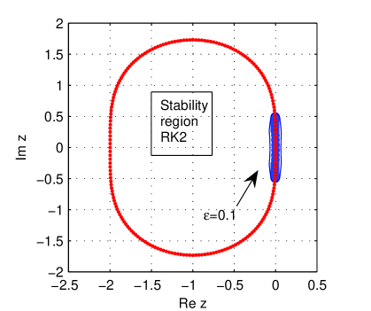
In order to validate the MoL for stiff problems we have depicted in Fig. 8 the pseudospectrum of corresponding to Thus we can conclude that MoL remains stable.
The same conclusion remains valid when the problem (15) is solved by SC coupled with Runge-Kutta higher than or AB of order . The pseudospectrum for is provided in Fig. 9.
The numerical solution for BBM-B problem (15) with the same initial data as above is depicted in Fig. 10.
It is rather difficult to compare Fig. 2 and Fig. 10 in order to grasp the meaning of the diffusive term on the wave propagation. However, a breaking up phenomenon of the initial wave persists despite the lost of the solution smoothness. From numerical point of view the stiffness introduced by this term makes the time marching process more slow.
We conclude this section with two remarks. Firstly, the spectra of the discrete operators and are almost rectilinear sets of points lying on the ordinate axis, or very close to it, and well included in the interval But this interval is the stability region for the leap frog scheme. Thus, this scheme is a possible candidate for a stable MoL.
Secondly, the above strategy extends directly to the more general equations of the form
where the linear operator belongs to a class of pseudo-differential operators and to BBM equation supplied with a forcing term or with slightly modified asymptotic conditions for the initial front.
5 Concluding remarks
In a sense, this study has succeeded in illustrating numerically the well established analytical and physical work [1]. Thus we have carried out solutions to a class of BBM Cauchy’s problems which inherit the smoothness properties of the initial front, conserve the energy invariant, are uniformly bounded over time and numerically stable.
We have used neither the domain truncation nor the periodicity hypothesis as is usually done. Instead, we have exploited the advantages offered by the scaling factor attached to HC method. Thus, with an ”optimal” scaling factor the accuracy at which the energy integral is satisfied, at least for MoL based on scaled HC and RK4, has been considerably improved. The spectral properties of the linearized spatial discretization operator have been tuned up in order to justify the stability of the MoL algorithm. Eventually the space-time domain has been enlarged such that the wave evolution is plainly observable. Additionally, the time integration period has been arbitrarily large which is fairly important from practical point of view.
Consequently, we honestly believe that we have added two important examples which confirm the fact that the Trefethen’s rule of thumb provides accurate predictions at least in the case of quasi normal matrices. We also believe that we have provided a solid argument for the validity of the BBM equation as a physical approximation of the dispersion of long waves.
References
- [1] Benjamin, T.B., Bona, J.L., Mahony, J.J., Model Equations for Long Waves in Nonlinear Dispersive Systems, Philos. Trans. Roy. Soc. London Ser.A., 272(1972) 47-78
- [2] Bona, J.L., Pritchard, W.G., Scott, L.R., Comparison of Two Model Equations for Long Waves, AMS Lectures in Applied Mathematics, 20(1983) 235-267
- [3] Boyd, J.P., Chebyshev and Fourier Spectral Methods, 2nd Ed., DOVER, 2000
- [4] D., Dutykh, T., Katsaounis, D., Mitsotakis, Finite volume schemes for dispersive wave propagation and runup, J. Comput. Phys., 230 (2011), 3035-3061
- [5] Funaro, D., Polynomial Approximation of Differential Equations, Springer Verlag, Berlin, 1992
- [6] Gheorghiu, C.I.: Laguerre collocation solutions to boundary layer type problems. Numer. Algor. 64, 385-401 (2013)
- [7] Gheorghiu, C.I.: Pseudospectral Solutions to some Singular Nonlinear BVPs. Applications in Nonlinear Mechanics. Numer. Algor. doi: 10.1007/s11075-014-9834-z
- [8] Gheorghiu, C.I., Spectral Methods for Non-Standard Eigenvalue Problems. Fluid and Structural Mechanics and Beyond, Springer Briefs in Mathematics, 2014
- [9] Higham, D.J., Trefethen, L.N., Stifness of ODEs, BIT, 33(1993) 285-303
- [10] Kassam, A-K., Trefethen, L.N., Fourth-Order Time Stepping for Stiff PDEs, SIAM J. Sci. Comp., 26 (2005) 1214–1233.
- [11] Marshall, H.G., Boyd, J.P., Solitons in a Continuously Stratified Equatorial Ocean, J. Phys. Oceanogr., 17 (1987) 1016-1031
- [12] Olver, F. W. J., Lozier, D. M., Boisvert, R. F., Clark, C. W., eds. , NIST Handbook of Mathematical Functions, Cambridge University Press, 2010
- [13] Omrani, K., The convergence of fully discrete Galerkin approximations for the Benjamin-Bona-Mahony (BBM) equation, Appl. Math. Comput., 180 (2006) 614-621
- [14] Omrani, K., Ayadi, M., Finite Difference Discretization of the Benjamin-Bona-Mahony-Burgers Equation, Numer. Methods Partial Differential Eq., 24 (2008) 239-248
- [15] Quarteroni, A., Saleri, F., Scientific Computing with MATLAB and Octave, 2nd Ed., Springer, 2006
- [16] Reddy, S.C., Trefethen, L.N., Stability of the method of lines, Numer. Math., 62(1992) 235-267
- [17] Stenger, F., Summary of Sinc numerical methods, J. Comput. Appl. Math., 121(2000) 379-420
- [18] Trefethen, L.N., Spectral Methods in MATLAB, SIAM, 2000
- [19] Wahlbin, L., Error estimates for a Galerkin method for a class of model equations for long waves, Numer. Math. 23 (1975) 289-303
- [20] Weideman, J.A.C., Reddy, S. C., A MATLAB Differentiation Matrix Suite, ACM Trans. on Math. Software, 26 (2000) 465–519
[1] T.B. Benjamin, J.L. Bona, J.J. Mahony, Model equations for long waves in nonlinear dispersive systems, Philos. Trans. Roy. Soc. London Ser.A. 272 (1972) 47–78.
[2] J.L. Bona, W.G. Pritchard, L.R. Scott, Comparison of two model equations for long waves, AMS Lect. Appl. Math. 20 (1983) 235–267.
[3] J.P. Boyd, Chebyshev and Fourier Spectral Methods, 2nd, DOVER, 2000.
[4] D. Dutykh, T. Katsaounis, D. Mitsotakis, Finite volume schemes for dispersive wave propagation and runup, J. Comput. Phys. 230 (2011) 3035–3061.
[5] D. Funaro, Polynomial Approximation of Differential Equations, Springer Verlag, Berlin, 1992.
[6] C.I. Gheorghiu, Laguerre collocation solutions to boundary layer type problems, Numer. Algor. 64 (2013) 385–401.
[7] C.I. Gheorghiu, Pseudospectral solutions to some singular nonlinear BVPs, Appl. Nonlinear Mech. Numer. Algorithm. (2015), doi:10.1007/s11075-014-9834-z
[8] C.I. Gheorghiu, Spectral Methods for Non-Standard Eigenvalue Problems. Fluid and Structural Mechanics and Beyond, Springer Briefs in Mathematics, Springer, Cham Heidelberg New York Dordrecht London, 2014.
[9] D.J. Higham, L.N. Trefethen, Stifness of ODEs, BIT 33 (1993) 285–303.
[10] A.-K. Kassam, L.N. Trefethen, Fourth-order time stepping for stiff PDEs, SIAM J. Sci. Comp. 26 (2005) 1214–1233.
[11] H.G. Marshall, J.P. Boyd, Solitons in a continuously stratified equatorial ocean, J. Phys. Oceanogr. 17 (1987) 1016-1031.
[12] F.W.J. Olver, D.M. Lozier, R.F. Boisvert, C.W. Clark (Eds.), NIST Handbook of Mathematical Functions, Cambridge University Press, 2010.
[13] K. Omrani, The convergence of fully discrete Galerkin approximations for the Benjamin-Bona-Mahony (BBM) equation, Appl. Math. Comput. 180 (2006) 614–621.
[14] K. Omrani, M. Ayadi, Finite difference discretization of the Benjamin-Bona-Mahony-Burgers Equation, Numer. Methods Partial Differential Eq. 24 (2008) 239–248.
[15] A. Quarteroni, F. Saleri, Scientific Computing with MATLAB and Octave, 2nd Ed., Springer, Springer-Verlag Berlin Heidelberg, 2006.
[16] S.C. Reddy, L.N. Trefethen, Stability of the method of lines, Numer. Math. 62 (1992) 235–267.
[17] F. Stenger, Summary of Sinc numerical methods, J. Comput. Appl. Math. 121 (2000) 379–420.
[18] L.N. Trefethen, Spectral methods in MATLAB, SIAM (2000).
[19] L. Wahlbin, Error estimates for a Galerkin method for a class of model equations for long waves, Numer. Math. 23 (1975) 289–303.
[20] J.A.C. Weideman, S.C. Reddy, A MATLAB differentiation matrix suite, ACM Trans. Math. Software 26 (2000) 465–519.