Abstract
The paper is devoted to obtaining accurate numerical solutions to some third-order nonlinear boundary problems on the real semi-axis of Blasius type. It aims to address these issues more accurately as boundary value problems rather than converting them into initial value problems. The Blasius boundary layer problem with slip and nonslip boundary conditions, the Sakiadis and FalknerSkan problems, a pseudoplastic boundary layer problem, etc, are solved using the Chebyshev technology, in the form of Chebfun, along with the domain truncation. The choice of this method is justified vis-à-vis the difficulties of solving some singular and nonlinear third-order boundary value problems. The convergence rate and the convergence order of Newton’s method in solving the nonlinear algebraic system obtained by discretisation are established. The shear stress is accurately estimated along with the first and second derivatives of the solutions. Some comments on the stability of numerical outcomes concerning the length of the integration domain are provided. The results are presented graphically and tabulated for the most challenging case (non-linearity involving fractional power). The method correctly captures the large gradients of the solution.
Authors
Calin-Ioan Gheorghiu
Tiberiu Popoviciu Institute of Numerical Analysis, Romanian Academy, Romania
Keywords
accurate; chebfun; solutions; third-order; nonlinear; BVPs; Chebyshev collocation
Paper coordinates
C.I. Gheorghiu, Accurate Chebfun solutions to third-order nonlinear BVPs on the half-line. Applications in boundary layer theory, Physica Scripta, 2025, https://doi.org/10.1088/1402-4896/adc51a
About this paper
Print ISSN
1402-4896
Online ISSN
google scholar link
Paper (preprint) in HTML form
Accurate Chebfun Solutions to Third-Order Nonlinear BVPs on the Half-Line. Applications in Boundary Layer Theory.
Abstract
The paper is devoted to obtaining accurate numerical solutions to some third-order nonlinear boundary problems on the real semi-axis of Blasius type. It aims to address these issues more accurately as boundary value problems rather than converting them into initial value problems. The Blasius boundary layer problem with slip and nonslip boundary conditions, the Sakiadis and Falkner-Skan problems, a pseudoplastic boundary layer problem, etc. are solved using the Chebyshev technology, in the form of Chebfun, along with the domain truncation. The choice of this method is justified vis-à-vis the difficulties of solving some singular and nonlinear third-order boundary value problems. The method’s convergence rate and the convergence order of Newton’s method in solving the nonlinear algebraic system obtained by discretisation are established. The shear stress is accurately estimate along with solutions’ first and second derivatives. Some comments on the stability of numerical outcomes with respect to the length of the integration domain are provided. The results are presented graphically and tabulated for the most challenging case (non-linearity involving fractional power). The method correctly captures the large gradients of the solution.
Keywords: Blasius equation, fractional power non-linearity, Chebyshev collocation, Chebfun, convergence, accuracy, shear stress.
1 Introduction
”Never solve a PDE when an ODE will do, and never solve a boundary value problem when an initial value problem will do”, a very interesting opinion expressed in the paper [1] and valid until the beginning of this century at the latest.
However, high-order (accuracy) numerical methods, such as spectral collocation, based on Chebyshev or other polynomials, encourage us to contradict at least the second part of this statement.
This is also the purpose of this paper, to show that boundary value problems (BVP), even if they are nonlinear and defined on an unbounded domain (the real semi-axis), can be solved without having to transform them into initial value problems (IVP). Moreover, we will establish the convergence of these methods, which have done little by reducing BVP to IVP. For this purpose, we will solve a set of seven problems that have challenging Blasius’ equation as a central model.
It is well-known that accurate numerical methods for solving BVPs are in high demand in various branches of physics and engineering. This aspect is well argued by a physicist in the paper [2]. Physicists and engineers are looking for accurate methods for solving singular BVPs that capture sharp and rapid changes in flow fields. We will try to answer at least partially to these desires. The BVPs below model viscous flows over various obstacles in which some physicochemical effects may also occur.
There are three essential difficulties in solving Blasius-type problems. The first consists of the introduction of the double boundary condition in origin, the second is given by the poor conditioning of the third-order differentiation matrices when using FD, FEM or conventional (classical) spectral collocation methods and finally, the slowness of the Newton iterations when solving nonlinear algebraic systems with full matrices.
These difficulties have been signalized and analyzed in turn by Wornom [3] (1978), Streett, Zang and Hussaini [4] (1984) and Canuto, Hussaini, Quarteroni and Zang (1988) [5] p. 188.
On the other hand, Chebfun by construction, just like the Chebyshev tau method, makes the introduction of any linear boundary condition a trivial matter. Most importantly, the Chebfun (chebop) system takes the next step and overloads linear operators via lazy evaluation (a functional programming facility) of spectral differentiation matrices. The consequences are better-conditioned systems such that Newton’s iterations can generally go faster.
We don’t even talk about shooting methods because they simply became obsolete after a long period in which they produced some results.
How Chebfun solves the three difficulties exposed above makes it attractive and broadens its applicability to practically BVP of any order. This is also the motivation we choose this strategy to the detriment of more known others.
It is important to note that conventional (classical) spectral collocation methods work traditionally, i.e. truncate the solution at a given resolution and then solve the problem. On the other hand, Chebfun works the other way around, uses larger and larger resolutions and truncates the solution only when the desired accuracy is reached, usually close to the precision of the computing machine.
It should also be noted that we have successfully approached by Chebfun some singular second-order BVPs in the paper [6] and the study of fourth-order BVPs is in visible progress.
Taking into account the shape of the integration domain, in our previous paper [7] we tried to solve various Blasius-type systems by Laguerre collocation (LC), Laguerre Gauss Radau collocation (LGRC), and Chebyshev mapping. The results were only partially satisfactory. Collocation was implemented in this work in the conventional (classical) sense. From what we will see below, the Chebfun results are superior.
To implement Chebfun we will do a truncation of the domain to the finite domain . We will comment on optimising the length of the integration domain in Subsection 2.2.
It is unanimously accepted that FD methods, particularly FEM have difficulties dealing with nonlinearities of the form or By contrast, Chebfun treats these nonlinearities with appreciable accuracy, mainly due to the lazy evaluations of differentiation matrices.
The remainder of the paper is as follows. The next section introduces the typical mathematical problem and provides some fundamental aspects of the strategy of the Chebfun programming environment. Section 3 is divided into six subsections, each devoted to a specific problem. These problems can differ in the equations that define them and sometimes the attached boundary conditions. Section 4 is devoted to solving a nonlinear system of two equations, the first of order three and the second of order two, modelling the flow in a boundary layer of a viscous incompressible fluid in a magnetic field. Finally, Section 5 states our belief that BVPs, even if they are non-linear and defined on unbounded domains, can be more accurately solved without transforming them into IVPs and then solved by various obsolete shooting algorithms. Some other conclusions that can be drawn from the paper and a brief perspective of its future are displayed in this Section.
2 On the Chebfun strategy
2.1 Mathematical formulation of the problem
Mathematically, we will have to solve the following nonlinear boundary value problem:
| (1) |
where is a third-order nonlinear differential operator of the form,
which may also possibly depend on some real parameters. The right-hand side member is a continuous function of all its arguments, and , and are specified constants.
Each smooth solution to the problem (1) is mapped to the interval and represented by an expansion in Chebyshev polynomials of the form
| (2) |
where is a natural number, the so called the resolution, and are the well known Chebyshev polynomials.
When constructing a solution (Chebfun object), the system computes the coefficients by interpolating the target function at Chebyshev’s extreme points,
| (3) |
The polynomial degree is automatically determined so that the above representation is as accurate as possible in double-precision arithmetic.
Polynomial interpolation in Chebyshev nodes is known to be near-optimal for approximating functions that are smooth, converging geometrically for analytic functions. The Fast Fourier transforms (FFTs) can be used to map function values to coefficients and vice versa, in operations.
The construction process actually begins by sampling the target function at points, with . The optimal degree is then determined such that is close to zero, relative to the coefficient of largest magnitude, for all
2.2 On the Chebfun programming environment
Chebfun is quite thoroughly described in the monographs of L. N. Trefethen and his students [8] and [9] (see also http://www.chebfun.org ). The motto under which this programming environment is further built is ”feel symbolic but run at the speed of numerics”. The aim of this open-source object-oriented MATLAB package is to achieve for functions what floating-point arithmetic achieves for numbers.
The fundamental principle of the Chebfun system is to evaluate functions in sufficiently many Chebyshev nodes (3) for a polynomial interpolant to be accurate to machine precision. Whenever the function of interest is only defined implicitly, as the solution of a differential equation, Chebfun works similarly with MATLAB based on collocation in the Chebyshev nodes and lazy evaluation of the associated spectral differentiation matrices.
This programming environment has proven to be very performing but sometimes encounters difficulties when the analyzed non-linearity contains rational (fractional) powers. To overcome this inconvenience, we initiated a method of continuation, that is, we solved simpler samples that do not contain such powers, whose solutions then became initial data for more complex problems.
To prove the convergence of the solution it is very valuable the estimation
| (4) |
which gives us a measure of how accurately Chebfun performed. Final error estimates for differential equations and boundary conditions are provided separately. They are generally better than the error defined by (4).
The error introduced with the formula (4) will help us to find an optimal length of the integration interval. This will be done for each example below without explicitly mentioning it.
To have precise definitions for classifying the rate of convergence of Chebfun in solving various problems, we refer to the well-known monograph of [10] (Section 2.3). Roughly, an expansion (series) of type (2) is said to have the property of supergeometric, geometric, or subgeometric convergence depending upon whether;
| (5) |
In a log-linear plot, vs., it is relatively simple to distinguish between these three types of convergence. We will do this for each of the examples below.
A very useful example of Chebfun’s code is found in our contribution [11]. There we solved a singular nonlinear BVP of the third order that accepts a prime integral and comes from the simulation of the large-scale circulation in an ocean (the Gulf Stream).
3 Blasius boundary layer type problems
3.1 Blasius equation along with nonslip boundary conditions
Let us consider the Blasius equation
| (6) |
along with the impermeability of the wall, the nonslip and the free stream velocity outside the boundary layer, respectively, boundary conditions
| (7) |
where the primes denote differentiation concerning the independent variable
Here we merely note that the function represents, after suitable normalization, the fluid velocity parallel to the wall (the Ox axis) and stands for normalized stream function. This problem is frequently dealt with in fluid dynamics textbooks but very rarely solved as a BVP.
Roughly, this problem describes the steady two-dimensional laminar boundary layer that forms on a semi-infinite plate which is held parallel to a constant unidirectional flow.
As a member of the Chebfun team, the author of [12] shows that the solution to this problem is a smooth, monotonically increasing function that rapidly converges to a linear polynomial away from the origin. The singularity of this solution is established at .
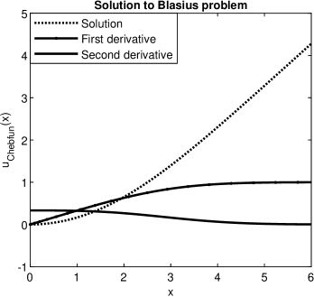
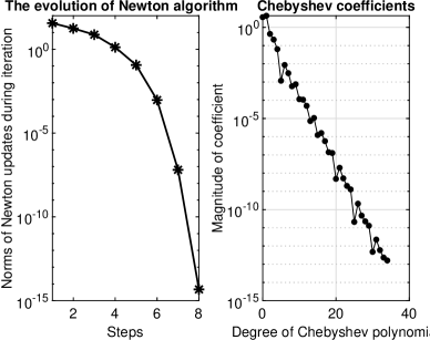
Our Chebfun solution along with its first two derivatives is depicted in Fig. 1. From the left panel of Fig.2 we infer that Newton’s method has second order and from the right panel of the same figure we can state that the convergence of spectral method tends to a geometric one. How the coefficients decrease is a correct indication of the convergence of the solution.
However, from the fifth line of Table 1 we see that the numerical value of the second derivative of solution in origin, the so-called the local shear stress, reaches the exact value computed in [13].
3.2 Blasius equation along with slip boundary conditions
We now attach to the Blasius equation (6) the following slip boundary condition
| (8) |
where is a non-dimensional parameter.
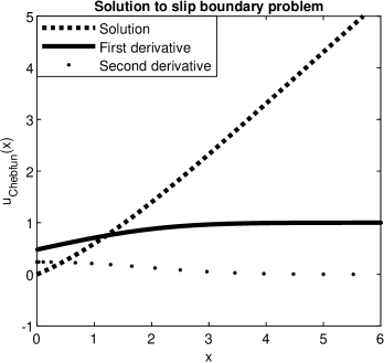
In our computations, we have used and obtained local shear stress Chebfun needed a modest resolution and provided the solution with an accuracy of order in iterations.
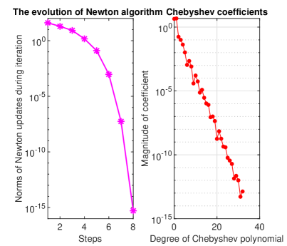
The solution to this problem is depicted in Fig. 3 and the convergence is argued in Fig. 4. It is visible from the second figure that the Newton method is second-order and the convergence of the solution is clearly geometric.
The length of the integration domain has been but for in the range we have obtained almost identical numerical results, i.e., that differs by less than
It is really surprising to note that the behaviour of a certain type of electromechanical energy converter (EMEC) is governed by the same Blasius equation (6) (see [14]). However, the behaviour of the solutions to the EMEC problem is essentially different from the boundary layer solution because of different initial and boundary conditions. It is not our purpose to analyze IVPs so we will not dwell on this problem.
3.3 The Sakiadis problem
The laminar boundary-layer behavior on a moving continuous flat surface is now investigated. We are concerned now with the classical Blasius equation (6) for the flat plate of infinite length along with the boundary conditions
| (9) |
(see also the paper of Sakiadis [15]).
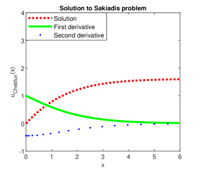
For this problem, Chebfun worked with in (2) in order to get an accuracy of order and Newton’s method has carried out the solution in iterations. The local shearing stress obtained, equals the value
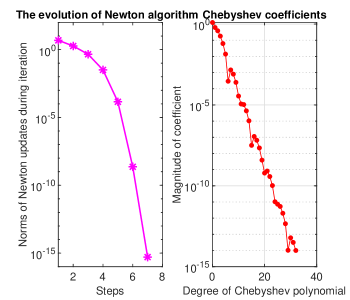
The Chebfun solution for this problem along with its first two derivatives is depicted in Fig. 5. From the left panel of Fig. 6 we observe that Newton’s method has an order less than two but close to this value and from the right panel of the same figure we can state that the convergence of spectral method tends to a geometric rate.
3.4 The Falkner-Skan problem
The well-known Falkner-Skan problem reads
| (10) |
where is a real parameter (wedge angle). It generalizes Blasius’ flow to wedge flow, i.e. flows in which the plate is not parallel to the flow.
The existence of a solution to the problem (10) when was first proved by Weyl in [16] and the uniqueness for is analyzed in Craven and Peletier, see [17].
For this problem, Chebfun worked with in (2) in order to get an accuracy of order and Newton’s method has carried out the solution in iterations with a convergence rate of order
The assumed value for has been and the local shearing stress obtained equals the value
| (11) |
There are two important sources by which we can verify this value. The first is due to [18] who shows that this value must be between and which happens for the value found by Chebfun.
Moreover, by a simple integration of the Falkner-Skan equation and the introduction of the boundary conditions from (10), the following important relationship is found in [19]
| (12) |
Chebfun calculates the two integrals simply and elegantly, and the value found for shear stress with (12) coincides with the exact one (11) up to the sixth decimal place.
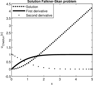
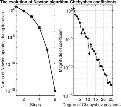
The solution to the problem (10) is depicted in Fig. 7 and details about the convergence of Newton’s method and the solution can be found in Fig. 8. It is clear that Newton’s method is of second order and the convergence of the solution approaches the geometric order.
3.5 The pseudoplastic boundary layer problem
In this section, we will be concerned with the problem classified as difficult, namely
| (13) |
with a sub-unit parameter. In his paper [20] Liao considers that this problem is a challenging nonlinear one for numerical techniques.
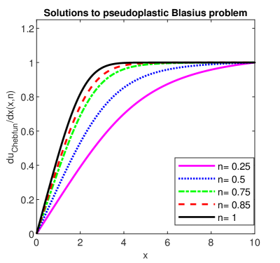
We want to note from the beginning that, a direct approach to this issue using Chebfun, led to a failure. Chebfun warns that the Newton method failed and asks for a better initial guess.
In this situation, we resorted to a kind of continuation, i.e. we first solved the problem with i.e. Blasius problem, and then we used its solution as an initial guess for the problem with an arbitrary .
The results are presented in Table 1 and a set of five solutions are presented in Fig. 9. It is observed that the error in the calculation of the solutions is of an order of or better. The order of the Newtonian method has not been reported, but it tends towards two in every case.
The numerical results have been stable for lengths
-
n Error (4) N (2) Iterations Convergence 1/4 1.987373418945310e-01 1.166735835465708e-08 31 6 geometric 1/2 2.785695654574897e-01 8.553189221841424e-09 39 6 geometric 3/4 3.767441379066853e-01 3.590474867116297e-08 41 6 subgeometric 4/5 3.962121166851580e-01 4.353691014663887e-08 42 5 subgeometric 1.0 3.320573357325587e-01 6.738127708134982e-09 35 8 geometric
3.6 Boundary-layer flows induced by permeable stretching walls
Along with Magyari and Keller [21], we consider the singular nonlinear BVP
| (14) |
| (15) |
where corresponds to an impermeable wall, to suction and to lateral injection of the fluid through a permeable wall. The coefficient comes from the power-law variations of the stretching velocity.
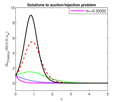
In our numerical experiments, the assumed value for has been For this value, in [21] the authors find an exact solution with the maximum value of its first derivative of Our numerical solutions reported in Fig. 10 visibly confirm this estimation.
Heidel in [22] observes that equation (14) differs only slightly from the Falkner-Skan equation (10). However, a basic difference between (14) and the Falkner-Skan equation is that the former is invariant under the transformation whereas the Falkner-Skan equation is not. This allows the reduction order of (14).
A fully analogous problem from [23] has been solved. To save space, we do not present these results.
4 A system of boundary layer type
4.1 The boundary layer for a rotating flow interacting with an axial magnetic field.
King and Lewellen consider in [25] the following singular BVP, i.e. the nonlinear differential system
| (16) | |||||
along with boundary conditions
| (17) | |||||
where is the power of the radius in the asymptotic assumption of external axial velocity and is a physical parameter proportional with the intensity of the magnetic field ( is assumed).
Physically, equations (16), with the boundary conditions of equation (17), determine the velocities in the boundary layer as a function of the similarity variable and the two parameters and .
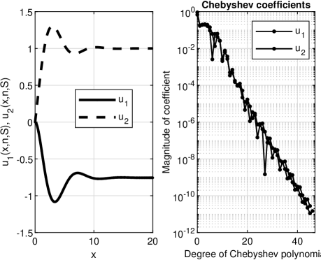
Our numerical results are depicted in Fig. 11. They have been obtained for but are perfectly stable for In fact, the value was also used in the work [24]. Unfortunately, a direct and quantitative comparison with these results is almost impossible to track. However, the allure of the variation of the unknowns and are the same.
It is interesting to note that an elementary solution of the system is given by the pair , and the parameter affects only the linear part of this system. Our numerical experiments confirm those from the paper [25] which observe that for , the oscillations of and are damped out and the thickness of the boundary layer drastically decreases.
5 Concluding remarks
Chebfun has proven to be a very effective and accurate method for solving the seven challenging problems exposed above. Sharp and rapid variations in flow field variables have been correctly captured.
All the problems addressed, model phenomena that come from fluid mechanics and physics. These are flows over certain obstacles, even permeable, accompanied by magnetic or viscoelastic effects.
The physics outcomes, i.e., the shape and velocity of the boundary layer and the local shear stress are correctly computed in all situations.
Some numerical or theoretical results unanimously accepted in the literature have been confirmed (see Subsection 3.1, Subsection 3.6, etc.) and some completely new ones have been provided (see Subsection 3.4, Subsection 3.5).
However, it is difficult to compare the resolution of a BVP at all points simultaneously (a ”jury” problem) with its resolution as an IVP, solved by a step-wise procedure (a ”marching” problem), especially when the second method does not produce an error analysis and the first method does.
This is also the reason why we could not compare the local shear stress values obtained with Chebfun with corresponding values widespread in the literature and obtained by shooting.
All in all, in this paper, we have provided credible numerical results for Blasius-type boundary value problems, supported by rigorous error analysis (see additionally our paper [26]).
The future goal of this paper is to be a step towards solving nonlinear and singular BVPs as easily with functions in the 21st century as we learned to do with numbers in the 20th (see also https://www.chebfun.org).
References
- [1] Boyd J P 1999 Exp. Math. 8 381
- [2] Abarzhi S I and Goddard III W A 2019 Proc Natl Acad Sci USA 116 18171. https://doi.org/10.1073/pnas.1818855116
- [3] Wornom S F 1978 NASA T P-1302 (Hampton, Virginia)
- [4] Streett C L, Zang T A and Hussaini M Y 1984 AIAA Pap. No. 84-0170
- [5] Canuto C, Hussaini M Y, Quarteroni A and Zang T A 1988 Spectral Methods in Fluid Dynamics, Springer-Verlag New-York Inc.
- [6] Gheorghiu C I 2022 Computation 10 116. https://doi.org/10.3390/computation10070116
- [7] Gheorghiu C I 2016 Numer. Algor. 73 1 https://doi.org/10.1007/s11075-015-0083-6
- [8] Driscoll T A, Hale N and Trefthen L N 2014 Chebfun Guide, 1st Edition, For Chebfun version 5.
- [9] Trefthen L N, Birkisson A and Driscoll T A 2018 Exploring ODEs, (Philadelphia, PA:SIAM)
- [10] Boyd J P 2000 Chebyshev and Fourier Spectral Methods, Dover Publications, Inc. 31 East 2nd Street, Mineola, New York 11501
- [11] Gheorghiu C I 2020 A third-order nonlinear BVP on the half-line https://www.chebfun.org/examples/ode-nonlin/GulfStream.html
- [12] Hrothgar 2014 Blasius function. https://www.chebfun.org/examples/ode-nonlin/Blasius.html, last accessed June 08, 2024
- [13] Boyd J P 2008 SIAM Rev. 50 791
- [14] Treve Y M 1967 SIAM J. APPL. MATH. 15 1209
- [15] Sakiadis B C 1961 AIChE J. 7 221
- [16] Weyl H 1942 Ann. of Math. 43 381
- [17] Craven A H, Peletier L A 1972 Mathematika 19 129
- [18] Coppel W A 1960 Phil. Trans. R. Soc. Lond. A 253 101 https://doi.org/10.1098/rsta.1960.0019
- [19] Sachdev P L, Kudenatti R B and Bujurke N M 2008 Stud. Appl. Math. 120 1
- [20] Liao S J 2005 J. Comput. Appl. Math. 181 467
- [21] Magyari E and Keller B 2000 Eur. J. Mech. B - Fluids 19 109
- [22] Heidel J W (1973) ZAMM 53 167
- [23] Klemp J B, Acrivos A 1976 J. Fluid Mech. 76 363
- [24] Holt J F 1964 Commun ACM 7 366
- [25] King, W S and Lewellen W S 1964 Phys Fluids 7 1674
- [26] Gheorghiu C I 2023 J.Phys.A: Math. Theor. 56 17LT01 (6pp) https://doi.org/10.1088/1751-8121/acc6a9
[1] Boyd J P 1999 Exp. Math. 8 381, Crossref, Google Scholar
[2] Abarzhi S I and Goddard W A III 2019 Proc Natl Acad Sci USA 116 18171, Crossref, Google Scholar
[3]Wornom S F 1978 Report Number: NASA-TP-1302 OL5335066A 1, Google Scholar
[4] Streett C L, Zang T A and Hussaini M Y 1984 AIAA J AIAA Paper 84-0170 1, Crossref, Google Scholar
[5] Canuto C, Hussaini M Y, Quarteroni A and Zang T A 1988 Spectral Methods in Fluid Dynamics (Springer-Verlag), Google Scholar
[6] Gheorghiu C I 2022 Computation 10 116, Crossref, Google Scholar, View PDF
[7] Gheorghiu C I 2016 Numer. Algor. 73 1, Crossref, Google Scholar
[8] Driscoll T A, Hale N and Trefthen L N 2014 Chebfun Guide, 1st Edition, For Chebfun version 5, Google Scholar
[9] Trefthen L N, Birkisson A and Driscoll T A 2018 Exploring ODEs (SIAM), Crossref, Google Scholar
[10] Boyd J P 2000 Chebyshev and Fourier Spectral Methods 2nd edn (Dover Publications, Inc), Google Scholar
[11] Gheorghiu C I 2020 A third-order nonlinear BVP on the half-line https://www.chebfun.org/examples/ode-nonlin/GulfStream.html,, Google Scholar
[12] Hrothgar 2014 Blasius function https://www.chebfun.org/examples/ode-nonlin/Blasius.html last accessed June 08 2024
Google Scholar
[13] Boyd J P 2008 SIAMRev 50 791, Crossref, Google Scholar
[14] Treve Y M 1967 SIAM J. APPL. MATH. 15 1209, Crossref, Google Scholar
[15] Sakiadis B C 1961 AIChE J 7 221, Crossref, Google Scholar
[16] Weyl H 1942 Ann. of Math 43 381, Crossref, Google Scholar
[17] Craven A H and Peletier L A 1972 Mathematika 19 129, Crossref, Google Scholar
[18] Coppel W A 1960 Phil. Trans. R. Soc. Lond. A 253 101, Crossref, Google Scholar
[19] Sachdev P L, Kudenatti R B and Bujurke N M 2008 Stud. Appl. Math. 120, Google Scholar
[20] Liao S J 2005 J.Comput. Appl. Math 181 467, Crossref, Google Scholar, View PDF
[21] Magyari E and Keller B 2000 Eur. J. Mech. B – Fluids 19 109, Crossref, Google Scholar
[22] Heidel J W 1973 ZAMM 53 167, Crossref, Google Scholar
[23] Klemp J B and Acrivos A 1976 J. Fluid Mech. 76 363, Crossref, Google Scholar
[24] Fang T and Zhang J 2008 Int. J. Non-Linear Mech. 43 1000, Crossref, Google Scholar
[25] King W S and Lewellen W S 1964 Phys Fluids 7 1674, Crossref, Google Scholar
[26] Holt J F 1964 Commun ACM 7 366, Crossref, Google Scholar
[27] Gheorghiu C I 2023 J. Phys. A: Math. Theor. 56 17LT01, Crossref, Google Scholar