Abstract
The aim of this paper is to show that the Jacobi–Davidson (JD) method is an accurate and robust method for solving large generalized algebraic eigenvalue problems with a singular second matrix. Such problems are routinely encountered in linear hydrodynamic stability analysis of flows that arise in various areas of continuum mechanics. As we use the Chebyshev collocation as a discretization method, the first matrix in the pencil is nonsymmetric, full rank, and ill‐conditioned. Because of the singularity of the second matrix, QZ and Arnoldi‐type algorithms may produce spurious eigenvalues. As a systematic remedy of this situation, we use two JD methods, corresponding to real and complex situations, to compute specific parts of the spectrum of the eigenvalue problems. Both methods overcome potentially severe problems associated with spurious unstable eigenvalues and are fairly stable with respect to the order of discretization. The real JD outperforms the shift‐and‐invert Arnoldi method with respect to the CPU time for large discretizations. Three specific flows are analyzed to advocate our statements, namely a multicomponent convection–diffusion in a porous medium, a thermal convection in a variable gravity field, and the so‐called Hadley flow.
Authors
C.I. Gheorghiu
-Tiberiu Popoviciu Institute of Numerical Analysis, Romanian Academy
J. Rommes
NXP Semiconductors, Eindhoven, The Netherlands
Keywords
Cite this paper as:
C.I. Gheorghiu, J. Rommes, Application of the Jacobi-Davidson method to accurate analysis of singular linear hydrodynamic stability problems. Int. J. Numer. Meth. Fluids, 71 (2013) 358-369.
References
see the expansion block below.
About this paper
Journal
Int. J. Numer. Meth. Fluids
Publisher Name
DOI
Print ISSN
?
Online ISSN
?
MR
?
ZBL
?
Paper (preprint) in HTML form
Application of the Jacobi-Davidson method to accurate analysis of singular linear hydrodynamic stability problems
Abstract
The aim of this paper is to show that the Jacobi-Davidson method is an accurate and robust method for solving large generalized algebraic eigenvalue problems with a singular second matrix. Such problems are routinely encountered in linear hydrodynamic stability analysis of flows which arise in various areas of Continuum Mechanics. As we use the Chebyshev collocation as a discretization method the first matrix in the pencil is nonsymmetric, full rank and ill-conditioned. Due to the singularity of the second matrix, QZ and Arnoldi type algorithms may produce spurious eigenvalues. As a systematic remedy of this situation we use two Jacobi-Davidson (JD) methods, corresponding to real and complex situations, in order to compute specific parts of the spectrum of the eigenvalue problems. Both methods overcome potentially severe problems associated with spurious instable eigenvalues and are fairly stable with respect to the order of discretization. The real outperforms the ARPACK method with respect to the CPU time for large discretizations. Three specific flows are analyzed in order to advocate our statements, namely a multi-component convection diffusion in a porous medium, a thermal convection in a variable gravity field and so the called Hadley flow.
1 Introduction
In a linear hydrodynamic stability analysis one first considers the linearization of the governing equations around a steady-state flow. The perturbation variables are described by a linear system of coupled differential equations supplied with a set of boundary conditions. The discretization of this system frequently leads to some non-Hermitian generalized eigenvalue problems with singular second order matrix in pencil. This fact was first observed in [1] in connection with stability of convective motion in a variable gravity field, in [2] where the authors analyze the stability of convective flows in porous media and in [3, 4, 5] where the authors consider various physical situations such as thermal convection in a box, a multi-component convection-diffusion and the Hadley flow. The same phenomenon is noticed in [6, 7, 8] for various incompressible flows. When the linear stability analysis of two-phase flows and free-surface flows (in MHD) are considered, the presence of eigenvalue at infinity is observed in [9] and [10].
The level of discretization needed to describe accurately the perturbed fields gives rise to large matrices, i.e., of order of thousands. This large dimension of problems rules out the calculation of the entire spectrum: usually, only the leading eigenvalues (those with the largest or the smallest real part) are computed. Up to our knowledge, the method was used in quasitotality of generalized eigenvalue problems encountered in linear hydrodynamic stability, see [11] for one of the first applications of in this context. Our papers [12] and [13] are not an exception to this situation. Unfortunately, the method has the main drawback that its complexity is of order and due to large CPU times required it is hardly applicable to large problems. In order to eliminate non-physical eigenvalues in such non-Hermitian singular problems some ad-hoc methods were designed. For instance, in [8] the authors introduce a technique based essentially on the physics of the flow in order to eliminate these spurious eigenvalues. In [14] the authors use a transformation that maps the spurious eigenvalues to an arbitrary location in the complex plane. In [15] and [16] for spectral Galerkin and Chebyshev tau (Lanczos) respectively, the authors suggest practical tricks in order to remove the spurious modes. The authors of [6] obtain reliable results for the rightmost eigenvalue of Orr-Sommerfeld equation provided that a scale resolution assumption is fulfilled, i.e., the ration between the Reynolds number and the square of the cut-off parameter is ”small”.
Hence, there is need for a more specialized algorithm which computes only a few specific eigenvalues of the algebraic problem. In the case of hydrodynamic stability problems considered hereafter, one is typically interested in the eigenvalues closest to zero. Consequently, in this paper we propose to use (a real variant [17] of) the Jacobi-Davidson method [18] to solve the arising generalized eigenvalue problems. Advantages of the Jacobi-Davidson method are that it is applicable to large-scale eigenvalue problems and that it can deal with spurious eigenvalues at infinity [19]. Concerning the eigenvalues at infinity, in principle can also be hampered by their presence. However, by clever selection strategies this can be avoided. Furthermore, in the paper [19] on purification it is described how shift-and-invert/Cayley transformation strategies can be employed to avoid convergence to eigenvalues at infinity.
However, we want to stress that, up to our knowledge, the method has not been applied previously to these hydrodynamic stability problems and hence it is a novelty of our paper.
On the other hand, we are thoroughly aware of the existence of several methods designed to compute a specified subset of eigenspectrum, such as Krylov based methods (see the paper of Golub and van Loan [20] for the main research developments in the area). The reason we use consists in the expertise we have got working with this method.
A partially similar study with ours is that of Valenttaro et al. [21]. The authors solve a two-dimensional eigenvalue problem by spectral collocation based on Legendre and Chebyshev polynomials. The generalized eigenvalue problem is solved by a Krylov subspace type method (incomplete Arnoldi-Chebyshev). For this method a detailed analysis of round-off error is provided. But, while our study refers to singular pencils Valenttaro et al. considers regular pencils.
The paper is organized as follows. In Section 2, we first introduce a linear hydrodynamic stability problem, comment on its weak and minimization formulations, and use the strategy from [12] to transform it into a second order system supplied with Dirichlet boundary conditions. By Chebyshev collocation the generalized algebraic eigenvalue problem is obtained. Then, a second and a third singular problems are discretized with the same strategy. In Section 3, the Jacobi-Davidson method is described. Numerical experiments are reported in Section 4 along with comments concerning the convergence and round-off errors involved. Conclusions are contained in Section 5.
2 Three specific singular linear hydrodynamic stability problems
In [12] the following even order eigenvalue problem was considered:
| (1) |
| (2) |
In these equations, as well as in the following two problems, stands for the derivative with respect to the variable . is the Rayleigh number which represents the eigenparameter of the problem (1)-(2), is the wavenumber, and are the amplitudes of the vertical velocity and temperature perturbation and signifies the gravity variation in the layer of fluid.
In order to reduce the order of differentiation in this problem we introduce the new variable
| (3) |
Consequently, the two point boundary value problem (1)-(2) can be rewritten as a second order system
| (4) |
supplied with the homogeneous Dirichlet boundary conditions
| (5) |
It is important to observe that the problem (1)-(2) can also be formulated as a sixth order differential equation
| (6) |
supplied with the hinged boundary conditions, namely
| (7) |
A weak formulation for the new problem (6)-(7) reads: find and such that
| (8) |
where the set is a closed subspace of defined by
More than that, the critical Rayleigh number can be characterized by the following minimization problem
| (9) |
whenever the quantity remains positive. In fact, in all our experiments this condition is fulfilled.
The strategy implemented with Chebyshev collocation method to solve the problem (4)-(5) leads to the following generalized eigenvalue problem
| (10) |
where the matrices and are
| (11) |
The submatrices and stand respectively for the second order differentiation matrix on the Chebyshev nodes of the second kind the unitary matrix of order and the matrix with all zero entries of order , being as usual the spectral (cut-off or resolution) parameter. They have the same significance in the forthcoming two problems. The matrix signifies the diagonal matrix . It is important to underline that in the differentiation matrix the boundary conditions are enforced, thus the rows and columns corresponding to the first node and the last node are deleted. All the differentiation matrices we have used come from [22]. The matrix is singular of rank
As a second test problem we consider another representative singular hydrodynamic stability problem. In this case we solve an eight order differential system which models multi-component convection-diffusion in a porous medium. Defining to be the wavenumber and the eigenparameter, the non-dimensional linear perturbation equations read ([4]):
| (12) |
supplied with the boundary conditions:
| (13) |
In the system (12), , , , are the perturbations of velocity, temperature and two solutes, and are thermal and solute Rayleigh numbers, respectively, and are salt Prandtl numbers, . Eventually signifies a quantity connected with the temperature of the upper boundary. The strategy casts this problem into a generalized eigenvalue one with the matrices and defined as follows:
| (14) |
As a third test problem we consider the stability of the so called Hadley flow. It refers to convection in a layer of porous medium where the basic temperature field varies in the vertical (i.e. direction) as well as along one of the horizontal directions which is defined as direction. The nondimensional perturbation equations are ([4])
| (15) |
supplied with boundary conditions
| (16) |
In (15), and are respectively the third component of velocity and temperature field perturbations. The steady-state solutions have the form
where and are the horizontal and vertical Rayleigh numbers, respectively, with and being the and wavenumbers and is the eigenparameter. The same strategy casts this problem into a generalized eigenvalue one with the matrices and defined as follows:
| (17) |
where , and is the first order differentiation matrix. We finish this section with the remark that the problem (15)-(16) can be reduced to a fourth order one in containing the leading term
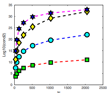
Our strategy is strongly motivated by the conditioning of the matrices , and its second, third and fourth powers. In Fig. 1 the log of the condition numbers of these matrices is depicted. In logarithmic terms, this picture shows that conditioning of the fourth order differentiation matrix doubles, and that conditioning of the sixth order differentiation matrix triples, the conditioning of second order matrix. The conditioning of the eighth order differentiation matrix is (roughly) only times larger than that of second order differentiation matrix. It means powers two, three or , of the conditioning of second order differentiation matrix, for the conditioning of higher order differentiation matrices, respectively. It is the main reason for which we do not applied directly collocation scheme to the problem (6)-(7) or to its weak formulation (8) or even to its minimization formulation (9). A completely analogous remark holds for the problems (12)-(13) and (15)-(16).
3 Computing a few specific eigenvalues
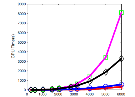
As mentioned in the introduction, the major drawback of full space methods such as the method (for ordinary eigenvalue problems) and the method (for generalized eigenvalue problems) [23] is their computational complexity of , where is the dimension of the problem. Consequently, for , direct computation of the complete spectrum is no longer feasible using the or method (see the uppermost curve in Fig. 2).
On the other hand, for the application described in this paper (and for many other applications as well), one is not interested in the complete spectrum, but in a few specific eigenvalues: the eigenvalues closest to zero. In fact the eigenvalue closest to zero is the most important. Before describing the proposed algorithm, first the requirements for an eigensolution method for the application of this paper are summarized:
-
1.
Given the number of wanted eigenvalues and a target (e.g., closest to zero), the methods must produce eigenvalues closest to the target.
-
2.
The method must be scalable with respect to the dimension of the eigenvalue problem.
-
3.
The method must produce real approximate values for real eigenvalues and complex (conjugated pairs of) approximate values for complex eigenvalues.
- 4.
In the following we briefly describe the Jacobi-Davidson method [18], an iterative method for the computation of a few specific eigenvalues. We also show why this method satisfies the above requirements. For more details, see [24, 18, 17].
3.1 The Jacobi-Davidson method
The Jacobi-Davidson method [18] combines two principles to compute eigenpairs of eigenvalue problems . The first (Davidson) principle is to apply a Ritz-Galerkin approach with respect to the search space spanned by the orthonormal columns of :
which leads to Ritz pairs , where are eigenpairs of . The second (Jacobi) principle is to compute a correction orthogonal to the selected eigenvector approximation (for instance, corresponding to the largest Ritz value ) from the Jacobi-Davidson correction equation
The search space is expanded with (an approximation of) . A Ritz pair is accepted if is smaller than a given tolerance. The basic Jacobi-Davidson method is shown in Alg. 1. A variant for generalized eigenvalue problems is described in [24].
If the correction equations are solved exactly, Jacobi-Davidson is an exact Newton method [25, 18], but one of the powerful properties of Jacobi-Davidson is that it is often sufficient for convergence to solve the correction equation up to moderate accuracy only, using, for instance, a (preconditioned) linear solver such as GMRES [26]. For our applications, however, the linear systems arising in the correction equation can be solved exactly in an efficient way. Jacobi-Davidson QR (QZ) methods, that compute partial (generalized) Schur forms for standard (generalized) eigenproblems, are described in [24, 25].
Reflecting on the requirements listed above, the Jacobi-Davidson method is known to be able to satisfy requirements 1 and 2. In the following subsection we describe how the other two can be dealt with.
3.2 Computing a partial generalized real Schur form
The Jacobi-Davidson QZ (JDQZ)[24] method for generalized eigenvalue problems computes a partial generalized Schur form [23]
| (18) |
where contain the generalized Schur vectors and are upper triangular matrices whose generalized eigenvalues are approximations (called Petrov values) of eigenvalues of . Note that .
Although the JDQZ method can be used for the problem described in this paper, there is one property that makes JDQZ in its current form less applicable: while the matrices and are known to be real, and hence have real or complex-conjugated pairs of eigenvalues, the produced partial Schur form is complex. In principle this should not be an issue. However, JDQZ does not guarantee that approximations to real eigenvalues are real, which could lead to confusion when computing eigenvalues of large systems. In other words, because approximations of real eigenvalues might in fact be complex-conjugated pairs of eigenvalues (with negligible though nonzero imaginary part), this could lead to wrong conclusions in practice.
In [17] a variant of JDQZ, called rJDQZ, is proposed that computes partial generalized real Schur form for then pencil :
| (19) |
where contain the generalized Schur vectors, is upper triangular, and is quasi-upper triangular (i.e., the diagonal contains a entry for real eigenvalues and a block for complex-conjugated pairs of eigenvalues). The generalized eigenvalues are approximations (called Petrov values) of eigenvalues of . Note again that .
The key difference between JDQZ and rJDQZ is that the latter uses only real search spaces, while JDQZ uses complex search spaces. Since rJDQZ uses real search spaces, the approximate eigenvalues are either real or appear in complex-conjugated pairs, which is in line with requirement 3. Apart from this, it was shown in [17] that because less complex arithmetic is used in rJDQZ, the method is also faster and more memory efficient compared to JDQZ.
Finally, since we are interested in the eigenvalues closest to zero, we do not expect any numerical problems caused by eigenvalues at infinity (requirement 4), as also described in [19]. However, when one is interested in, e.g., the rightmost finite eigenvalues, one might consider purification techniques described in [27, 19].
3.3 Alternatives
An alternative method to compute a few specific eigenvalues is the Arnoldi method [28]. Since the Arnoldi method was originally derived for ordinary eigenvalue problems of the form , it is not directly applicable to problems of the form (cf. (10)). However, if it is possible to solve systems , one can apply the Arnoldi method to the transformed problem , where . Note that is not inverted explicitly; during the Arnoldi process, instead systems are solved (for more details see, e.g., [29]). If solves with can be done efficiently and accurately, the Arnoldi method may be an interesting alternative for the Jacobi-Davidson method (note that the Jacobi-Davidson method is still applicable if solves with are not feasible).
For the problem at hand, the Arnoldi method is applicable because of the sparsity of matrix and relatively cheap solves with .
4 Numerical results
In this section we will report some representative numerical results obtained in solving the generalized algebraic eigenvalue problems defined by (10), (14) and (17). All numerical computations reported in [12] and [13] were carried out using the MATLAB code eig, which is an implementation of the QZ method. Alternatively, we use in this paper the implementation from
the implementation described in [17], and compare the results with those obtained using the MATLAB code eig for the method (see also Table 3 in [12]), and the MATLAB code for the Arnoldi method. All computations were carried out using MATLAB 2010a on a HP xw8400 Workstation with clock speed of 3.2Ghz/s.
The computed values of the first three eigenvalues, i.e. , corresponding to problems (10) and (14) respectively are displayed in Table 1. The eigenvalues corresponding to problem (17) are reported in Table 2. The CPU times reported in these tables, as well as in Fig. 2, measure the time required for the computation of the first six eigenvalues except QZ method which computes the whole spectrum.
They are obtained for the following sets of fixed physical parameters: , , , , , , , in case of problem (14), and in case of problem (10), and , , , , in case of problem (17).
It is fairly clear from both Tables that most numerical approximations of the first three leading eigenvalue computed by both , and Arnoldi are almost indistinguishable. Our numerical experiments concerning problem (14), the largest one, extended successfully for all four methods for larger values of spectral parameter , i.e., for in the range , . This involved matrices of order , i.e., up to . As the values of the first two eigenvalues, up to sixth digit, remain unchanged for such range of , it implies convergence of the numerical method.
The CPU times required by the all four methods are depicted in Fig. 2. It is important to observe that computed only the first two eigenvalues for spectral parameter larger than .
In spite of its considerable robustness for large matrices, failed to compute the first eigenvalue corresponding to problem (17) (see second column in Table 2). The reason consists in the very bad conditioning of problem defined by (17).
The real variant of , , does produce real eigenvalues because it uses real search spaces, as explained in Section 3.2.
Both Arnoldi and the based methods did not show any difficulties with spurious eigenvalues.
We also have to emphasize that, as far as we know, we have used the largest spectral order in such eigenvalue computations. Comparatively, in [2] and [4] values of attain , in [9] the authors work with of order , in [8] the authors consider that is fine enough to predict correctly the leading eigenvalues of the problem and in [6] this order attains . In older papers the authors simply work with much less than .
Some more comments on the convergence and round-off errors in and Arnoldi method when singular generalized eigenvalue problems are solved are now in order. We define first, the error of a method as the absolute value of the difference between the computed eigenvalue and the converged one, i.e., obtained with the largest resolution. Than, we observe that the pseudospectra of our pencils can be unbounded, i.e., they extend to the whole complex plane for sufficiently large perturbations (see van Doersselaer [30]). Thus, to get some information we cut up from the whole spectrum the region surrounding the first two eigenvalues and observe that our computation is backward stable in the sense that the line of level which equals the error encloses the computed eigenvalue. Using a resolution of which implies a matrix of order the pseudospectrum is depicted in Fig. 3.
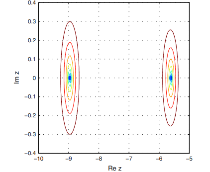
As the diameter of the enclosed area provides a hint of the largest possible relative error on the respective eigenvalue, we can infer a more sensitive second eigenvalue than the first one.
The errors of the first two computed eigenvalues, by and respectively Arnoldi, vs. , as is usual in spectral methods, are depicted in Fig. 4.
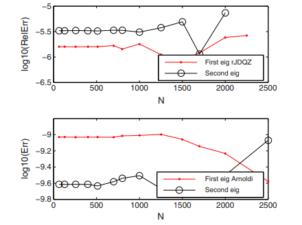
For resolutions larger than this picture shows that the computation of the second eigenvalue becomes unstable in both methods. It is in accordance with the conclusion provided by the pseudospectrum. In order to observe the order of convergence of both methods we depicted Fig. 5.
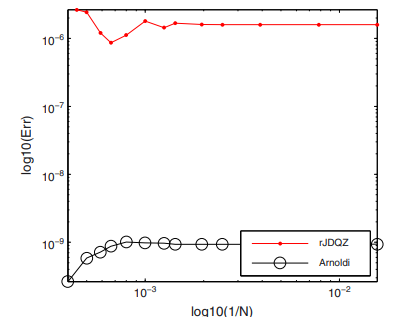
The method for resolutions inferior to have order of convergence that could attains unity, i.e., is of order . These resolutions are satisfactory in hydrodynamic stability problems. Arnoldi method behaves better. It has a comparable order of convergence but looks more accurate. It is fairly clear that method is seriously affected by rounding off errors in Chebyshev differentiation matrices.
With respect to Arnoldi method we have to observe that this method confirms its performances established in [21] also for generalized singular eigenvalue problems.
5 Concluding remarks
In this paper we have shown that the Jacobi-Davidson and Arnoldi methods can be successfully used to compute the smallest eigenvalues of large-scale matrix pencils arising in hydrodynamic stability problems.
Both methods are not hampered by eigenvalues at infinity. Since these methods are applicable to large-scale problems, they are preferred over the method, which is only applicable to small eigenvalue problems. The variant of the Jacobi-Davidson method that uses only real search spaces, , takes advantage of using such search spaces resulting in real approximations of real eigenvalues. Consequently, it is the fastest method for solving such large and singular generalized eigenvalue problems. Moreover, this method is completely independent of the physical formulation of the problem at hand.
Eventually, we want to underline that the Chebyshev collocation (discretization) method proved again to be very implementable and feasible, for fairly large values of spectral parameter, provided that accurate differentiation matrices are used.
Acknowledgement 1
The authors are very grateful to the anonymous referee for his/her careful reading of the paper and trenchant suggestions for improvement.
References
- [1] Straughan B. Convection in a variable gravity field. Journal of Mathematical Analysis and Applications, 1989; 140:467-475.
- [2] Straughan B, Walker DW. Two very accurate and efficient methods for computing eigenvalues and eigenfunctions in porous convection problems. Journal of Computational Physics, 1996; 127:128-141.
- [3] Dondarra JJ, Straughan B, Walker DK. Chebyshev tau-QZ algorithm methods for calculating spectra of hydrodynamic stability problems. Applied Numerical Methods, 1996; 22:399-434.
- [4] Hill AA, Straughan B. A Legendre spectral element method for eigenvalues in hydrodinamic stability. Mathematical Methods in Applied Sciences, 2006; 29 :363-381.
- [5] Hill AA, Straughan B. Linear and nonlinear stability tresholds for thermal convection in a box. Mathematical Methods in Applied Sciences, 2006; 29 :2123-2132.
- [6] Melenk JM, Kirchner NP, Schwab C. Spectral Galerkin discretization for hydrodynamic stability problems. Computing, 2000; 65:97-118.
- [7] Kirchner NP. Computational aspects of the spectral Galerkin FEM for the Orr-Sommerfeld equation. International Journal for Numerical Methods in Fluids, 2000; 32:119-137.
- [8] Valerio JV, Carvalho MS, Tomei C. Filtering the eigenvalues at infinity from the linear stability analysis of incompressible flows. Journal of Computational Physics, 2007; 227:229-243.
- [9] Boomkamp PAM, Boersma BJ, Miesen RHM, Beijnon GVA. A Chebyshev collocation method for solving two-phase flow stability problems. Journal of Computational Physics, 1997; 132:191-200.
- [10] Giannakis D, Fischer PF, Rosner R. A spectral Galerkin method for the coupled Orr-Sommerfeld and induction equations for free surface MHD. Journal of Computational Physics, 2009; 228:1188-1233, DOI:10.1016/j.jcp.2008.10.016
- [11] Khorrami MR, Malik MR, Ash LR. Application of spectral collocation techniques to the stability of swirling flows. Journal of Computational Physics, 1989; 81:206-229.
- [12] Gheorghiu CI, Dragomirescu IF. Spectral methods in linear stability. Application to thermal convection with variable gravity field. Applied Nunerical Mathematics, 2009; 59:1290-1302, DOI:10.1016/j.apnum.2008.07.004
- [13] Dragomirescu IF, Gheorghiu CI. Analitical and numerical solutions to an electrohydrodynamic stability problem. Applied Mathematics and Computation, 2010; 216:3718-3727, DOI:10.1016/j.acm.2010.05.028.
- [14] Schmid PJ, Henningson DS. Stability and Transition in Shear Flows. Springer-Verlag: New York, 2001; 489.
- [15] Zebib A. Removal of Spurious Modes Encountered in Solving Stability Problems by Spectral Methods. Journal of Computational Physics, 1987; 70:521-525.
- [16] Lindsay KA, Ogden RR. A Practical Implementation of Spectral Methods Resistant to the Generation of Spurious Eigenvalues. International Journal for Numerical Methods in Fluids, 1992;15:1277-1292.
- [17] van Noorden TL, Rommes J. Computing a partial generalized real Schur form using the Jacobi-Davidson method. Numerical Linear Algebra with Applications, 2007;14:197-215.
- [18] Sleijpen GL, van der Vorst HAA. A Jacobi-Davidson iteration method for linear eigenvalue problems. SIAM Journal of Matrix Analysis and Applications, 1996;17:401-425.
- [19] Rommes J. Arnoldi and Jacobi-Davidson methods for generalized eigenvalue problems with singular. Mathematics of Computation, 2008;77:995-1015.
- [20] Golub GH, Van der Vorst HA. Eigenvalue computation in the 20th century. Journal of Computational and Applied Mathematics, 2000; 123:35-65.
- [21] Valdettaro L, Rieutord M, Braconnier T, Fraisse V. Convergence and round-off errors in a two-dimensional eigenvalue problem using spectral methods and Arnoldi-Chebyshev algorithm. Journal of Computational and Applied Mathematics, 2007; 205:382-393.
- [22] Weideman, JAC, Reddy SC. A MATLAB Differentiation Matrix Suite. ACM Transactions in Mathematical Software, 2000;26:465-519.
- [23] Golub GH, van Loan CF. Matrix Computations. third ed., The John Hopkins University Press: Baltimore, 1996.
- [24] Fokkema DR, Sleijpen GLG, van der Vorst HA. Jacobi-Davidson style QR and QZ algorithms for the reduction of matrix pencils. SIAM Journal of Scientific Computing, 1998;20:94-125.
- [25] Sleijpen GLG, Booten JGL, Fokkema DR, van der Vorst. Jacobi-Davidson type methods for generalized eigenproblems and polynomial eigenproblems. BIT, 1996;36:595-633.
- [26] Saad Y, Schultz MH. GMRES: A generalized minimal residual algorithm for solving nonsymmetric linear systems. SIAM Journal of Scientific and Statistic Computing, 1986;7:856-869.
- [27] Meerbergen K, Spence A. Implicitely restarted Arnoldi with purification for the shift-invert transformation. Mathematics of Computation, 1997;66:667-689.
- [28] Arnoldi WE. The principle of minimized iteration in the solution of the matrix eigenproblem. Quartely of Applied Mathematics, 1951;9:17-29.
- [29] Bai Z, Demmel J, Dongarra J, Ruhe A, van der Vorst HA. Templates for the Solution of Algebraic Eigenvalue Problems: a Practical Guide. SIAM:Philadelphia, 2000.
- [30] van Dorsslaer JLM. Pseudospectra for matrix pencils and stability of equilibria. BIT, 1997; 37:833-845
| JDQZ | rJDQZ | eig (QZ) | eigs (Arnoldi ) | |
|---|---|---|---|---|
| JDQZ | rJDQZ | eig (QZ) | eigs (Arnoldi ) | |
- Straughan B. Convection in a variable gravity field. Journal of Mathematical Analysis and Applications 1989; 140:467–475.
- Straughan B, Walker DW. Two very accurate and efficient methods for computing eigenvalues and eigenfunctions in porous convection problems. Journal of Computational Physics 1996; 127:128–141.
- Dondarra JJ, Straughan B, Walker DK. Chebyshev tau-QZ algorithm methods for calculating spectra of hydrodynamic stability problems. Applied Numerical Methods 1996; 22:399–434.
- Hill AA, Straughan B. A Legendre spectral element method for eigenvalues in hydrodinamic stability. Mathematical Methods in Applied Sciences 2006; 29:363–381.
- Hill AA, Straughan B. Linear and nonlinear stability tresholds for thermal convection in a box. Mathematical Methods in Applied Sciences 2006; 29:2123–2132.
- Valerio JV, Carvalho MS, Tomei C. Filtering the eigenvalues at infinity from the linear stability analysis of incompressible flows. Journal of Computational Physics 2007; 227:229–243.
- Boomkamp PAM, Boersma BJ, Miesen RHM, Beijnon GVA. A Chebyshev collocation method for solving two-phase flow stability problems. Journal of Computational Physics 1997; 132:191–200.
- Giannakis D, Fischer PF, Rosner R. A spectral Galerkin method for the coupled Orr–Sommerfeld and induction equations for free surface MHD. Journal of Computational Physics 2009; 228:1188–1233. DOI: 10.1016/j.jcp.2008.10.016.
- Khorrami MR, Malik MR, Ash LR. Application of spectral collocation techniques to the stability of swirling flows. Journal of Computational Physics 1989; 81:206–229.
- Gheorghiu CI, Dragomirescu IF. Spectral methods in linear stability. Application to thermal convection with variable gravity field. Applied Nunerical Mathematics 2009; 59:1290–1302. DOI: 10.1016/j.apnum.2008.07.004.
- Dragomirescu IF, Gheorghiu CI. Analitical and numerical solutions to an electrohydrodynamic stability problem. Applied Mathematics and Computation; 2010(216):3718–3727. DOI: 10.1016/j.acm.2010.05.028.
- Saad Y. Iterative Methods for Sparse Linear Systems. PWS Publishing: NY, 1996.
- Schmid PJ, Henningson DS. Stability and Transition in Shear Flows. Springer-Verlag: New York, 2001. 489.
- Zebib A. Removal of spurious modes encountered in solving stability problems by spectral methods. Journal of Computational Physics 1987; 70:521–525.
- Lindsay KA, Ogden RR. A practical implementation of spectral methods resistant to the generation of spurious eigenvalues. International Journal for Numerical Methods in Fluids 1992; 15:1277–1292.
- Melenk JM, Kirchner NP, Schwab C. Spectral Galerkin discretization for hydrodynamic stability problems. Computing 2000; 65:97–118.
- van Noorden TL, Rommes J. Computing a partial generalized real Schur form using the Jacobi–Davidson method. Numerical Linear Algebra with Applications 2007; 14:197–215.
- Sleijpen GL, van der Vorst HAA. A Jacobi–Davidson iteration method for linear eigenvalue problems. SIAM Journal of Matrix Analysis and Applications 1996; 17:401–425.
- Rommes J. Arnoldi and Jacobi–Davidson methods for generalized eigenvalue problems Ax D Bx with B singular. Mathematics of Computation 2008; 77:995–1015.
- Golub GH, Van der Vorst HA. Eigenvalue computation in the 20th century. Journal of Computational and Applied Mathematics 2000; 123:35–65.
- Valdettaro L, Rieutord M, Braconnier T, Frayssé V. Convergence and round-off errors in a two-dimensional eigenvalue problem using spectral methods and Arnoldi–Chebyshev algorithm. Journal of Computational and Applied Mathematics 2007; 205:382–393.
- Weideman JAC, Reddy SC. A MATLAB differentiation matrix suite. ACM Transactions in Mathematical Software 2000; 26:465–519.
- Golub GH, van Loan CF. Matrix Computations, third ed. The John Hopkins University Press: Baltimore, 1996.
- Fokkema DR, Sleijpen GLG, van der Vorst HA. Jacobi–Davidson style QR and QZ algorithms for the reduction of matrix pencils. SIAM Journal of Scientific Computing 1998; 20:94–125.
- Sleijpen GLG, Booten JGL, Fokkema DR, van der Vorst HA. Jacobi–Davidson type methods for generalized eigenproblems and polynomial eigenproblems. BIT 1996; 36:595–633.
- Saad Y, Schultz MH. GMRES: a generalized minimal residual algorithm for solving nonsymmetric linear systems. SIAM Journal of Scientific and Statistic Computing 1986; 7:856–869.
- Meerbergen K, Spence A. Implicitely restarted Arnoldi with purification for the shift-invert transformation. Mathematics of Computation 1997; 66:667–689.
- Arnoldi WE. The principle of minimized iteration in the solution of the matrix eigenproblem. Quartely of Applied Mathematics 1951; 9:17–29.
- Bai Z, Demmel J, Dongarra J, Ruhe A, van der Vorst HA. Templates for the Solution of Algebraic Eigenvalue Problems: A Practical Guide. SIAM: Philadelphia, 2000.
- van Dorsslaer JLM. Pseudospectra for matrix pencils and stability of equilibria. BIT 1997; 37:833–845.