Abstract
Concentration time series are provided by simulated concentrations of a nonreactive solute transported in groundwater, integrated over the transverse direction of a two-dimensional computational domain and recorded at the plume center of mass. The analysis of a statistical ensemble of time series reveals subtle features that are not captured by the first two moments which characterize the approximate Gaussian distribution of the two-dimensional concentration fields. The concentration time series exhibit a complex preasymptotic behavior driven by a nonstationary trend and correlated fluctuations with time-variable amplitude. Time series with almost the same statistics are generated by successively adding to a time-dependent trend a sum of linear regression terms, accounting for correlations between fluctuations around the trend and their increments in time, and terms of an amplitude modulated autoregressive noise of order one with time-varying parameter. The algorithm generalizes mixing models used in probability density function approaches. The well-known interaction by exchange with the mean mixing model is a special case consisting of a linear regression with constant coefficients.
Authors
M. Crăciun
-Tiberiu Popoviciu Institute of Numerical Analysis, Romanian Academy
C. Vamoș
-Tiberiu Popoviciu Institute of Numerical Analysis, Romanian Academy
N. Suciu
-Tiberiu Popoviciu Institute of Numerical Analysis, Romanian Academy
Keywords
Cite this paper as:
M. Crăciun, C. Vamos, N. Suciu, Analysis and generation of groundwater concentration time series, Advances in Water Resources, vol. 111 (2018), pp. 20-30
doi: 10.1016/j.advwatres.2017.10.039
About this paper
Print ISSN
0169-3913
Online ISSN
1573-1634
MR
?
ZBL
?
Google Scholar
Paper (preprint) in HTML format
Analysis and generation of groundwater concentration time series
Abstract
Concentration time series are provided by simulated concentrations of a nonreactive solute transported in groundwater, integrated over the transverse direction of a two-dimensional computational domain and recorded at the plume center of mass. The analysis of a statistical ensemble of time series reveals subtle features that are not captured by the first two moments which characterize the approximate Gaussian distribution of the two-dimensional concentration fields. The concentration time series exhibit a complex preasymptotic behavior driven by a nonstationary trend and correlated fluctuations with time-variable amplitude. Time series with almost the same statistics are generated by successively adding to a time-dependent trend a sum of linear regression terms, accounting for correlations between fluctuations around the trend and their increments in time, and terms of an amplitude modulated autoregressive noise of order one with time-varying parameter. The algorithm generalizes mixing models used in Probability Density Function approaches. The well-known Interaction by Exchange with the Mean mixing model is a special case consisting of a linear regression with constant coefficients.
keywords:
time series analysis , Monte Carlo simulations , global random walk , groundwaterMSC:
[2010] 37M10 , 65C05 , 60G50 , 86A051 Introduction
Time series are ubiquitous in all fields of hydrology. Monitoring strategies and sampling procedures in various water management contexts, as for example in monitoring of nutrients [1] or of nitrate transport in groundwater [2], are based on analyses of concentration time series obtained from geophysical observations. The most common examples of groundwater concentration time series are the breakthrough curves obtained from concentration measurements at reference planes in aquifers. Also often used in subsurface hydrology literature are series indexed, instead of time, by a one-dimensional spatial variable (see e.g. [3]). Examples of such series are, among others, measured data on porosity, permeability, hydraulic conductivity, electrical resistivity (see [4] and references therein). The complexity of the hydrological time series drew the attention of the scientific community long time ago. The analysis of long-run hydrological and other geophysical time series [5, 6] lead to new concepts extending the classical Gaussian models, such as Gaussian fractional noise and fractional Brownian motion [7]. During the last two decades, such mathematical objects were used in subsurface hydrology, notably to model the complex structure of the hydraulic conductivity [8, 9, 3]. These modeling approaches are based on both measured and synthetic time series. Synthetic time series obtained from numerical simulations can be used to investigate the behavior of some quantities which are not accessible to direct measurements. For instance, it was shown, by using an automatic algorithm to decompose time series into intrinsic components, that in some conditions the transverse component of the trajectory of the classical advection-dispersion model of transport in heterogeneous aquifers with randomly distributed hydraulic conductivity behaves as a fractional Brownian motion or even as a multifractal [10].
Concentration time series recorded at regular time intervals at given points of the aquifer system supply observational data for monitoring and risk assessments of groundwater quality. In the context of stochastic subsurface hydrology, the heterogeneity of the groundwater flow domain is modeled as a random environment. Consequently, predictions on the behavior of the contaminant concentration are uncertain and have to be modeled as random functions. In discrete representations, a random function is equivalent to an ensemble of random time series recorded at different points in the domain. Risk assessments are based on the Probability Density Function (PDF) of the random concentration. Concentration PDFs can be inferred, in case of moderate heterogeneity, if one assumes a Gaussian shape of the concentration with random spatial moments estimated from the statistics of the random hydraulic conductivity [11], or by assuming the shape of the concentration PDF itself [12]. In recent years there were several attempts to apply the PDF approach from turbulence modeling [12, 13] to problems of stochastic subsurface hydrology [14, 15, 16, 17].
The PDF approach consists of solving a PDF evolution equation, which can be derived from the advection-dispersion-reaction equation verified by the random concentration [12]. Evolution equations with the same structure are obtained in the Filtered Density Function (FDF) approach where, instead of ensemble averages, spatial filtering procedures are used to infer statistical quantities [17]. Such equations have to be parameterized by using closure hypotheses and models. While the transport of the concentration PDF in the physical space can be modeled by known upscaling procedures, building a “mixing model” which describes the transport of the PDF in the concentration space is still a challenging issue [17]. A possible way to search for appropriate mixing models is to use the numerical approach based on the Fokker-Planck equation describing the evolution of a suitably weighted concentration PDF [16]. In this approach, the mixing model for nonreactive transport is given by an ordinary stochastic differential equation describing the evolution of the concentration on trajectories of an advection-dispersion process. In case of reactive transport with species-independent diffusion coefficients, chemical reactions are modeled by including in the stochastic differential equation drift terms given by reaction rates [17, Eq. (5)]. In this study, we investigate the structure of an ensemble of synthetic random time series of concentration values recorded on the trajectory of the center of mass of the solute plume and we derive a stochastic process which generates time series with almost the same statistics. This process reveals the structure and provides the parameters of the mixing model which closes the PDF equation for the concentration at the plume center of mass.
Time series associated to the classical model of nonreactive transport were recently constructed by integrating over the transverse direction of a two-dimensional domain the concentration fields computed with the Global Random Walk (GRW) algorithm [18] at successive longitudinal coordinates of the plume center of mass. An ensemble of such time series was computed with independent realizations of the random velocity field and a PDF approach was developed to simulate the PDF of the random concentration [16, 17]. The mechanism responsible for the transport of the concentration PDF in concentration space is, in this case, the stochastic process which generates the ensemble of concentration time series. A simple mixing model inferred from the ensemble of simulated time series generates time series by summing up increments of a time-dependent trend and Gaussian white noise terms with decaying amplitude [17]. Though this PDF approach provides results close to reference Monte Carlo (MC) simulations at early times, its performance deteriorates at larger times. This can be attributed to the inability of the mixing model to reduce the spreading of the realizations of the process generating the time series around their ensemble average, necessary to produce the asymptotical narrowing of the concentration PDF shown by MC simulations.
Keeping in mind the utility of the concentration time series in designing mixing models for PDF approaches, we look for a stochastic model for the concentration time series that can be used to generate statistical ensembles having similar features with the initial ensemble of time series obtained from GRW-MC simulations.
In this paper, the simple model previously used in [17] is refined and modified by considering more complex time series increments. The correct asymptotic behavior is ensured by a linear dependence between distances of time series realizations to their ensemble average and their increments in time. In this way, the larger the distances from the ensemble average, the stronger the increments tend to reduce them. The residuals obtained after removing the linear regression are correlated and, as a first approximation, we model them with an amplitude modulated autoregressive process of order one (AR(1)) with time-varying parameter. Our modeling approach uses methods of time series theory [19, 20], where statistical inferences are obtained from individual time series, as well as methods of statistical physics, based on statistical ensembles [21].
The paper is organized as follows. In Section 2 the statistical ensemble obtained by GRW-MC simulations is described. Section 3 is dedicated to the analysis and modeling of the ensemble average of the time series and of the increments of the centered time series obtained by subtracting the ensemble average from each time series. In Section 4 we introduce the linear regression between the centered time series and their increments and we infer the regression coefficients. The demodulated regression residuals are further modeled as an AR(1) process with time-varying parameter in Section 5. In the last Section we present some conclusions and discuss the implications of the new time series model for mixing models in PDF methods. The influence of sampling time, spatial sampling domain, and hydraulic conductivity on the structure of the time series model is analyzed in A.
2 Statistical ensemble of concentration time series
We consider the two-dimensional problem for nonreactive transport in saturated aquifers, previously used in numerical investigations based on GRW simulations [22, 23, 24] and PDF approaches [16, 17]. The nonreactive transport was modeled as an advection-dispersion process with a constant isotropic local dispersion coefficient m2/d and advection velocity fields given by realizations of a random space function. For a log-normally distributed hydraulic conductivity field with small variance and isotropic Gaussian correlation with correlation length set to m, the velocity realizations were generated numerically as superpositions of random periodic modes with the Kraichnan routine [25] by the usual approximation for small variances of (see details in [17, Appendix A]). The mean velocity field with an amplitude m/d was aligned with the -axis.
The simulations were conducted over 4000 time steps d, which correspond to 2000 days or equivalently, to 2000 advection time scales . The computational domain was a rectangle with dimensions of 750 m in the longitudinal direction and 300 m in the transversal direction. A constant spatial step of 0.1 m was considered in both directions, so that the GRW lattice contained 22.5 millions of nodes. The computational domain was larger than the maximum extension of the plume and, every time when groups of particles reached the outflow boundary, the domain was displaced in the direction of the mean flow, so that it contained the entire plume at all times. Therefore, with this numerical setting no boundary conditions were necessary. The initial condition consisted of an instantaneous injection of particles, uniformly distributed in a transverse slab of 1 m 100 m. Details on the numerical implementation of the GRW algorithm can be found in [22]. The cross-section concentration recorded at the -coordinate of the expected center of mass of the solute plume, , was obtained by summing the number of particles over transverse slabs , where m and is the transverse dimension of the two-dimensional domain. For each simulation, one obtains in this way a time series
| (1) |
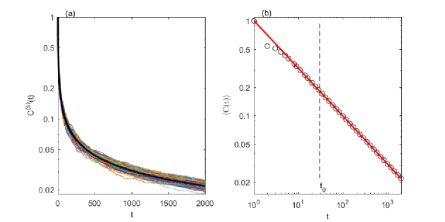
The concentrations were sampled at intervals , which correspond to one day. A statistical ensemble , , of time series of length was obtained by repeating the simulations for independent realizations of the velocity field (see Figure 1(a)).
In [22, Appendix B2] it has been shown that the large values of the parameters , , and used in our GRW-MC simulations ensure the reliability of the statistical inferences obtained by averaging over the ensemble . The simplified advection-dispersion model (constant, isotropic local dispersion coefficient and isotropic hydraulic conductivity with small variance) considered in this study is the same as that used to develop the PDF/FDF approach for groundwater systems [17]. Despite its simplicity, this model can be used to illustrate essential features of transport in groundwater, such as influence of local dispersion and sampling volume on concentration fluctuations [26, 28], ergodicity [22], memory effects [23], or anomalous behavior [10]. On the other hand, the transport of the cross-section spatially averaged concentration (1) is well approximated by a one-dimensional process parameterized by longitudinal components of the velocity and dispersion coefficients, as shown by the numerical results presented in [17, Section 5]. Hence, the behavior of the time series (1) is not affected by the anisotropy of the transport parameters as long as the longitudinal dispersion coefficient does not depend on transverse dispersion, for instance when the anisotropic dispersion coefficients are proportional to velocity or constant [26]. The choice of a small variance of the log-hydraulic conductivity facilitates the computation of large ensembles of time series with thousands of terms because it allows fast transport simulations with Kraichnan generated velocity fields, instead of numerical solutions of the flow equations, which would require huge computing resources.
It has been shown both theoretically [26, 27, 29] and numerically [28, 22] that for dispersion processes in random velocity fields with short-range correlation, non-vanishing mean, and small fluctuations, the concentration is approximately normally distributed, with time-decaying maximum concentration and concentration variance at the center of the plume. Moreover, in the long time limit the process approaches a Gaussian diffusion with constant coefficients, sometimes called “macrodispersion” process [22, 23].
The behavior of the ensemble average of the concentration sampled across the transverse dimension of the computational domain is accurately approximated by a one-dimensional diffusion process with drift velocity and a time variable ensemble dispersion coefficient [17]. In the long time limit, the normalized mean concentration is then given by the Gaussian probability density of the diffusion process with mean and constant macrodispersion coefficient ,
| (2) |
The mean concentration at the expected center of mass behaves in time as and, because of the approach to the macrodispersion process, it is an “attractor” for the time series investigated in this paper.
The transport in the concentration space of the concentration PDF investigated in [17] is governed by a mixing model describing the behavior of the increments of the time series process. A statistical analysis of 500 time series has been used to build a simple model for the increments , consisting of a deterministic trend given by the ensemble average and a “heteroskedastic process”, approximated by a white noise with time-decaying amplitude [17]. Numerical simulations using this mixing model gave good results at early and intermediate times but failed to predict the true concentration PDF at large times [16, 17, 24]. The observation that this simple mixing model does not describe the approach to the macrodispersive attractor was the starting point and the motivation for deeper investigations presented in this paper.
3 Statistical time series analysis and modeling
Each time series for fixed can be analyzed with methods of time series theory using statistical inferences obtained by time sampling and averaging (see for example [19, 20]). But if the time series have regions with strong-nonstationarity, like the concentration series investigated here, these methods fail to reveal some important features. In such cases, one can use the statistics of the ensemble for fixed and all values of . For example, the ensemble average of the concentration (see figure 1) is given by the arithmetic mean of the concentration values at given .
Figure 1(b) presents the log-log plot of the ensemble average of concentration as function of time. Its variation is almost linear except a few values at the beginning of the time series. These values may be associated with the numerical transition from the discontinuous initial condition (see Section 2) to a Gaussian shape of the two-dimensional concentration field in our GRW simulations. Therefore, we consider and fit the average with a power law function,
| (3) |
plotted with straight line in Fig. 1(b). The fit is consistent with the long time behavior of the concentration sampled at the plume’s center implied by (2). Even though the fit is already very good for , the restriction is necessary to obtain simple, power-law models for the amplitude of the increments of the time series which are analyzed in the following.
The centered time series are obtained by subtracting the ensemble average from each time series,
| (4) |
and their increments are defined by
| (5) |
The increments (5) shown in Fig. 2(a) are heteroscedastic, that is, their amplitudes vary with time. We denote by the ensemble average of the absolute values of the increment time series at given . By analogy to the theory of financial time series (see for example [30]), we refer to the mean amplitude as the “volatility” of the increment time series. Its values are plotted in log-log coordinates in Fig. 2(b). The logarithm of the volatility has a region with nonlinear variation at the beginning and, for , two distinct regions where its variation is almost linear with respect to , i.e. has a power law decay with respect to . In these regions has two different slopes (the absolute value of the first one being larger).
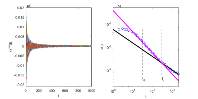
To determine more precisely the time value for which changes its slope, we consider a fixed initial time , a fixed end point and a variable intermediate time . For each value of we fit with linear functions for and for . We compute the square norm error for every value ,
which has a minimum at . This minimum separates the two regions with different slopes. So, we can divide the length of the time series into three distinct regions with different behavior of the volatility : a region with numerical variability from to ; a transient region where the volatility decreases rapidly and can be modeled by the power-law function , , between and ; a region which corresponds to the approach to the asymptotic behavior, with a slow decrease of the volatility, modeled by the power law function , , , between and .
In the following we analyze the residuals obtained after dividing every increment time series , of the statistical ensemble by the volatility ,
| (6) |
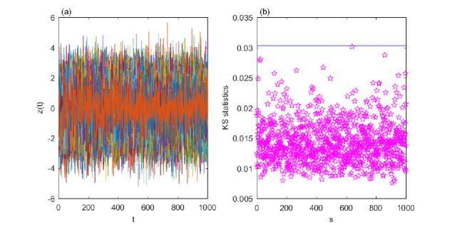
The residuals plotted in Fig. 3(a) seem to be realizations of an uncorrelated noise. Using a common approach in time series theory, we check whether the distribution of the residuals , for fixed and is normal by the Kolmogorov-Smirnov test. The statistics of this test is defined as the maximum of the absolute value of the difference between the empirical cumulative distribution function of the individual standardized residual series and the theoretical cumulative distribution function of the normal distribution (see for e.g. [31]). Figure 3(b) shows that all values are smaller than the critical value , which corresponds to a 5% significance level. The values of the autocorrelation functions, estimated through time averages on individual realizations, are already negligible from the first time lag. Together, these tests indicate that the residual process defined by (6) is a Gaussian white noise.
Based on the above analysis, the concentration time series can be modeled as a combination of a deterministic variation of power law type and a sum of terms generated by a Gaussian white noise modulated in amplitude. The relations (4-6) and the model of the volatility presented above, provide a relatively simple model of the concentration time series for ,
| (7) |
with average concentration and volatility modeled by
| (12) | |||||
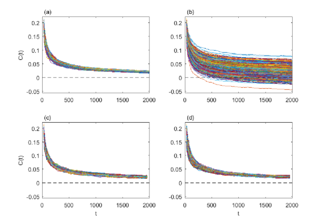
This model needs initial values for . The analysis of the ensemble , shows that the initial values are almost normally distributed with zero mean and variance . In order to verify this model we used (7-3) to generate concentration time series, plotted in Fig. 4(b). One observes that the time series generated with this model are much more scattered than the initial time series (Fig. 4(a)). Moreover, instead of approaching to zero for large values of , some generated time series take negative values. In conclusion, the model (7-3) fails to reproduce the behavior of the initial time series.
4 Modeling the asymptotic behavior of the concentration
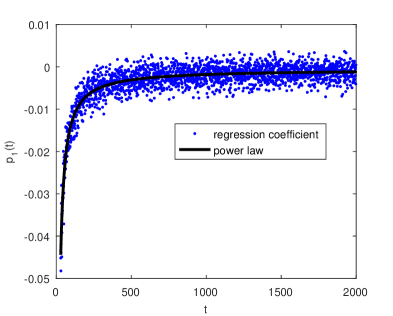
To account for the asymptotic behavior of the concentration time series in Fig. 4(a), the simple model defined by relations (7-3) has to be completed with a mechanism which prevents the scattering of the time series realizations shown in Fig. 4(b). That means, when the distance between a realization of the concentration time series and the ensemble average increases, it should be decreased at the next time steps by increments in the opposite direction. Therefore, we investigate the relation between and its increments at the next time steps by computing Pearson correlation coefficients through averages over the ensemble of time series realizations. The relevant, non-zero correlation is that between and the increments . The corresponding coefficient starts from negative values, followed by a rapid increase in time and an approach to zero through small fluctuations. The processes and are thus anticorrelated.
In the mean, the relation between the anticorrelated and , , is given by a linear regression with coefficients and . With being the fluctuating part of about the linear regression, the increments are advanced in time according to the model
| (13) |
Figure 5 presents the values of . One observes that they have high variability and most of the values are negative. Their dependence on time is well fitted with the power law function
| (14) |
The values of this function are used in the following as coefficients describing the dependence between and in the model of . The values of , not presented here, are very small (all being below ), so they will be neglected.
The fluctuations obtained after removing the values from , for , are still heteroscedastic, similar to the increments shown in Fig. 2(a). The corresponding volatility is given by the ensemble average and the residuals are defined, similarly to (6), by
| (15) |
The log-log plot of the volatility has two linear parts with different slopes. They are fitted with power law functions denoted by using the method described in the previous section,
| (16) |
We note that all the values of the coefficients in (16) are very close to those given in (3). Thus, removing the linear regression from does not change the volatility in a significant way. The Kolmogorov-Smirnov test and the autocorrelation functions indicate, again, that the residual process defined in (15) is a Gaussian white noise.
Taking into account the analysis from this section we modify the model (7) for the ensemble of concentration time series for as follows:
| (17) |
with defined in (3), given by Eq. (14), given by Eq. (16), initial values almost normally distributed with zero mean and variance , and , where .
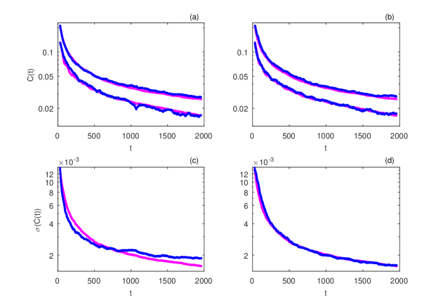
The regression between and introduced in (17) is the mechanism we were looking for, which ensures the convergence of the concentration time series towards the true asymptotic behavior. An ensemble of 1000 concentration time series generated with the model (17) is presented in Fig. 4(c). They now have a convergent behavior similar to that of the original ensemble (compare Fig. 4(a) and Fig. 4(c)). The minimum and maximum concentration values for the initial ensemble and of the generated one are also similar (see Fig. 6(a)). But the standard deviation estimated by averaging over the ensemble of generated time series is a bit smaller for , while for it is larger than for the initial ensemble (see Fig. 6(c)).
5 Nonstationarity of the residual time series
The residuals from relation (17) seem to be realizations of a Gaussian white noise. However, as seen in Section 3, statistical inferences based on time averages computed on individual time series could be misleading. Therefore, a deeper investigation on the statistical structure of the residuals time series should be carried out.
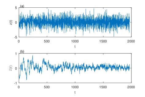
To proceed, we apply a symmetric moving average filter (see for example [32]) with the semi-length of the window equal to to every , for fixed (e.g. Fig. 7(a)). The resulted time series are inhomogeneous, with large amplitudes at early times, which slowly decay at large times (Fig. 7(b)). The inhomogeneity might be attributed to a nonstationary autocorrelation of the stochastic process .
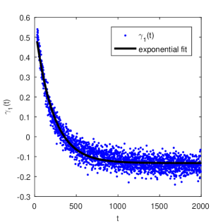
To investigate this possibility, we computed correlations between the residuals and , through averages over the ensemble of realizations, at time lags for all . The ensemble Pearson correlation coefficients for , denoted by , are plotted in Fig. 8. Over the first several hundreds time steps takes positive values, then, it decreases towards negative values and reaches an almost stationary regime at large times. The correlation coefficients for and are significantly smaller than and can be neglected. Hence, the process is a nonstationary correlated noise with correlation coefficient decreasing in time.
This analysis suggests that the residuals can be modeled in a first approximation as an AR(1) process with time-varying correlation coefficient (see e.g. [33, 34, 35]),
| (18) |
where . The variable correlation coefficients can be fitted with an exponential function with a constant added (plotted with continuous line in Fig. 8),
| (19) |
We also find that the initial values can be well approximated by a normal distribution with zero mean and .
Considering the AR(1) model for the residuals in (17), we obtain a complete model that can be used to generate concentration time series, specified by relations (17), (18) and (19). An ensemble of 1000 time series generated with this model is presented in Fig. 4(d). The corresponding minimum and maximum values of are shown in Fig. 6(b) and the standard deviations in Fig. 6(d). Figures 6(a) and 6(b) show that the extreme values of the concentration can be reproduced with either the white noise or the AR(1) models for residuals. Instead, the standard deviation of the concentration time series generated by using the AR(1) model (Fig. 6(d)) is much more accurate than that obtained with the white noise model (Fig. 6(c)).
To conclude the validation of the model (17-19), we also estimated the probability densities of the values of generated with the AR(1) noise model for residuals and compared them with those inferred from the initial ensemble MC-GRW simulations. The PDFs are close to each other at all times (those for , and are compared in Fig. 9), as already expected from the good results for extreme concentration values and standard deviations shown in Fig 6. As the time increases the PDFs get narrower and narrower, indicating that the values of fluctuate close to the average concentration and reach the correct asymptotic behavior. Thus, the time series generating process (17-19) has the desired features of an appropriate mixing model for the PDF approach proposed in [17].
A similar mixing model for FDF evolution equations can be derived from an ensemble of time series obtained from GRW-MC simulations based on spatially filtered Kraichnan velocity fields generated with the algorithm described in [17, Appendix A]. The practical advantage of the FDF approach is that the effect of sampling volume can be investigated without solving volume averaged transport equations because their solutions, e.g. volume averaged concentration and variance, can be readily obtained by computing the moments of the FDF solution.
6 Discussion and conclusions
The analysis of a statistical ensemble of 1000 time series of concentration allowed us to reveal their complex structure. The main structure is similar to a Brownian motion but modified by four types of nonstationarity. According to (3), the average concentration decreases as a power law, in agreement with the theoretical model (2) (this being the first nonstationarity of deterministic trend type). On this deterministic variation a random component (expressed as a sum of increments) is superposed (see (17)). If the increment time series were a Gaussian white noise, then the random component would be a Brownian motion. But the increment time series contains three nonstationarities: the increments are anticorrelated with the distance between the concentration and its average value over the statistical ensemble, anticorrelation described by the linear regression coefficient (14) which is varying in time; the amplitude of the residuals of the regression varies in time according to the volatility (16); moreover the demodulated regression residuals have a variable correlation in time and are modeled by an AR(1) process with a time-varying parameter (18).
The complexity of the structure of these time series also manifests itself in their convergence in time to the asymptotic self-similar evolution. For the simulated concentrations undergo a numerical transition as the discontinuous initial concentration is smoothed out. After this initial period of time, there is a transition period of about 300 time steps with a strong nonstationarity, where the volatility has a rapid decrease (Fig. 2), the linear regression coefficient is much larger in absolute value than at later times (Fig. 5) and the autoregressive correlation coefficient takes large positive values (Fig. 8). For larger values of , as the evolution of the concentration approaches the asymptotic behavior, all these parameters have small variations and tend to a stationary value.
Figure 4(b) illustrates the inability of the simple model (7-3), which is a precise mathematical formulation of the mixing model used in [17], to avoid the spreading of the ensemble of time series around the mean as the time increases. The behavior of the original ensemble (Fig. 4(a)) is reproduced with the new model (17) by considering the linear regression term, while keeping the noise term unchanged (Fig. 4(c)). By considering the AR(1) noise (18-19), the model (17) improves the overall convergent behavior of the ensemble of generated time series, as well as the estimation of the standard deviation.
A mixing model moves the PDF in concentration spaces by increments of concentration time series [12, 24, 16, 17]. Using (4), the increments of the time series model (17) can be written in a form closer to that used in PDF approaches:
| (20) |
The first and last terms in the right hand side correspond to the simple stochastic model (7) and to its empirical formulation in [17]. The linear regression (middle term) has the structure of Interaction by Exchange with the Mean (IEM) model used in PDF methods for turbulent flows [12]. The only difference is that instead of the variable coefficient , the factor in the IEM model is a constant, proportional to the “mixing frequency” (inverse of the characteristic time scale). The IEM model is an exact mixing model, rigorously derived for homogeneous and isotropic turbulence [13]. However, in PDF problems for transport in groundwater flows the IEM model underestimates the drift in concentration space which moves the PDF towards small concentration values [16, 17]. A time-dependent coefficient of the IEM model, heuristically inferred from the parameters of the transport problem, has been also proposed [29]. It improves the PDF simulation, but only for small to intermediate times. It seems that the drawback of the IEM model is the absence of the trend increment and that of the noise term. In case of the simple stochastic model (7), the drawback is the absence of the regression term. Both models are generalized by the complete time series model (17).
The model (17) reveals the structure of the mixing model which governs the transport in concentration space of the PDF of defined by Eq. (1). The transport of the concentration PDF in concentration space presented in Fig. 9 shows that the mixing model (20) is practically exact in this case. Similarly to the classical IEM model which is appropriate for modeling a large variety of scenarios of turbulent transport, one expects that mixing models for more complex problems of transport in groundwater will have the same structure as (20), consisting of a deterministic trend, a noise, and a regression term generalizing the classical IEM model. Since the variable regression coefficient in Eq. (14) is negative, the regression term describes the time-dependent relaxation of the fluctuations as the concentration approaches a spatially uniform distribution. Comparing Fig. 4(b) to Fig. 4(c) and Fig. 4(d), we can see that the presence of this term in (17) prevents the occurrence of negative concentrations, which is a major drawback of diffusion-like mixing models [12].
The large number of parameters of the model (17) is required to generate time series with approximately the same statistics as the initial ensemble (see Fig. 6 and Fig. 9). On the other hand, we found that using, instead of AR(1), autoregressive and moving average models of higher order with larger number of parameters to model the noise in (17) does not significantly improve the results. The need to fit a large number of parameters could be however a cumbersome task in practical applications to PDF/FDF problems. Moreover, these parameters are not directly related to the physical parameters of the transport problem. To parameterize a model with the same structure as in (20), but for different transport conditions and physical parameters, one needs another set of real data, i.e. an ensemble of time series realizations. For practical purposes of estimating PDFs of maximum concentration by the approach proposed in [17], the mixing model (20) can be parameterized, for the beginning, as follows: a trend given by the average concentration (2) at the plume center of mass, completely specified by the macrodispersion coefficient (or a similar expression for the average concentration at finite times, depending on the ensemble dispersion coefficient ); a white noise with variable amplitude, inferred from analyses of individual synthetical or measured time time series, for instance by using the automatic detrending algorithm presented in [32]; the IEM model with variable coefficients introduced in [29], specified by the local dispersion coefficient and the longitudinal component of the effective dispersion tensor or equivalently, by the longitudinal effective dispersion coefficient, the correlation length of the log-hydraulic conductivity field, and the dispersion time scale .
The time series mixing model (20) has been inferred from MC simulations for initial conditions which correspond to an instantaneous injection of the resident concentration in an experimental setup. We did not consider the in-flux injection mode and continuous injections over finite intervals in time or in the longitudinal spatial direction [36]. In such situations we only can expect that a stationary regime is reached more rapidly and the regression coefficient in Eq. (20) approaches a constant value in shorter times. We investigated instead the influence of the sampling time and spatial sampling domain, as well as the effect of large variance of the log-hydraulic conductivity field. In all cases we found that the time series process has the general structure of Eq. (20), but with more or less important changes of the parameters. As shown in A.1, the effect of reducing the sampling interval from 1 d to 0.5 d is the strengthening of the correlation of the noisy in Eq. (17). By replacing the transverse slab in Eq. (1) with square sampling domains of edge equal to 1 m and 2 m, respectively, we found that the regression coefficient is no longer a power law, being better approximated by a polynomial fitting and the numerical transition at the beginning of the time series takes longer, the model being valid for (A.2). Increasing the variance of the log-hydraulic conductivity field to , the time series model reproduces the statistics of the initial ensemble with a lower accuracy but still keeps the structure of (16) as well as the structure of the parameter functions, with modified numerical constants. Moreover, since larger velocity fluctuations result in enhanced mixing, the smoothing of the discontinuous initial condition is faster than for small variability, and the model is already valid for (A.3). As a general conclusion, we note that the time series model has a general structure consisting of a deterministic trend, a linear regression, and a noise, but for accurate assessments of the parameters separate analyzes for different experimental scenarios are required.
Acknowledgements
The computation of the ensemble of concentration time series was supported by the Jülich Supercomputing Centre–Germany as part of the Project JICG41. The work of N. S. was partially supported by the Deutsche Forschungsgemeinschaft–Germany under Grant AT 102/7-1, KN 229/15-1, SU 415/2-1.
Appendix A Influence of sampling time, spatial sampling domain, and variance of the field
A.1 Influence of sampling time
Repeating the analysis presented above for an ensemble of time series obtained from the same GRW-MC simulations but with cross-section concentration (1) sampled at 0.5 d, instead of 1 d, we found that the time series model preserves the structure (17), with modified parameters. As shown in Table 1, the model (3) of the mean concentration remains practically unchanged, the difference between the coefficients being a consequence of time scaling from to in case d, where the time series with terms corresponds to the same physical time of d. The other parameters are more or less close to each other, with the exception of the parameters of the AR(1) noise. The decrease of and the increase of in (19) correspond to a strengthening of the correlation of the noisy part of the increments from (17). Since this correlation is strictly positive in case , according to (17), the correlation of the centered time series (4) increases as well. These effects are somewhat similar to that observed in a recent study on the influence of the lag on the statistics of the increments of a subordinated Gaussian process [4].
| d | 1.0084 | 0.5053 | -1.3733 | 1.0127 | -5.5460 | 0.7021 | 0.0047 | -0.1321 |
| d | 1.3980 | 0.5021 | -0.8079 | 0.9389 | -6.4511 | 0.5589 | 0.0027 | 0.2364 |
A.2 Influence of spatial sampling domain
To investigate the dependence of the time series model on the sampling domain we repeated the analysis from Sections 3-5 for concentration time series sampled similarly to Eq. (1) at the expected center of mass of the plume at time intervals of one day, in spatial domains of 2m x 2m and 1m x 1m. The corresponding ensembles of GRW-MC simulations were obtained for the same numerical setup and initial condition of the two-dimensional transport problem as for the ensemble of concentration time series sampled in cross-section transverse slabs described in Section 2. The new time series are more irregular than those sampled in the cross section of the domain. This process is no longer an exact mixing model but can be used as a starting approximation for three-dimensional PDF problems (two spatial dimensions and a concentration axis).
The new time series models for small sampling domains keep the general structure of (17). But now the regression coefficient is no longer a power law function, being better approximated by a polynomial fitting. (For the purpose of illustrations presented in Figs. 1 and 2 we did not refine the polynomial fitting, using instead the regression coefficients computed from initial ensembles of time series smoothed with a moving average.)
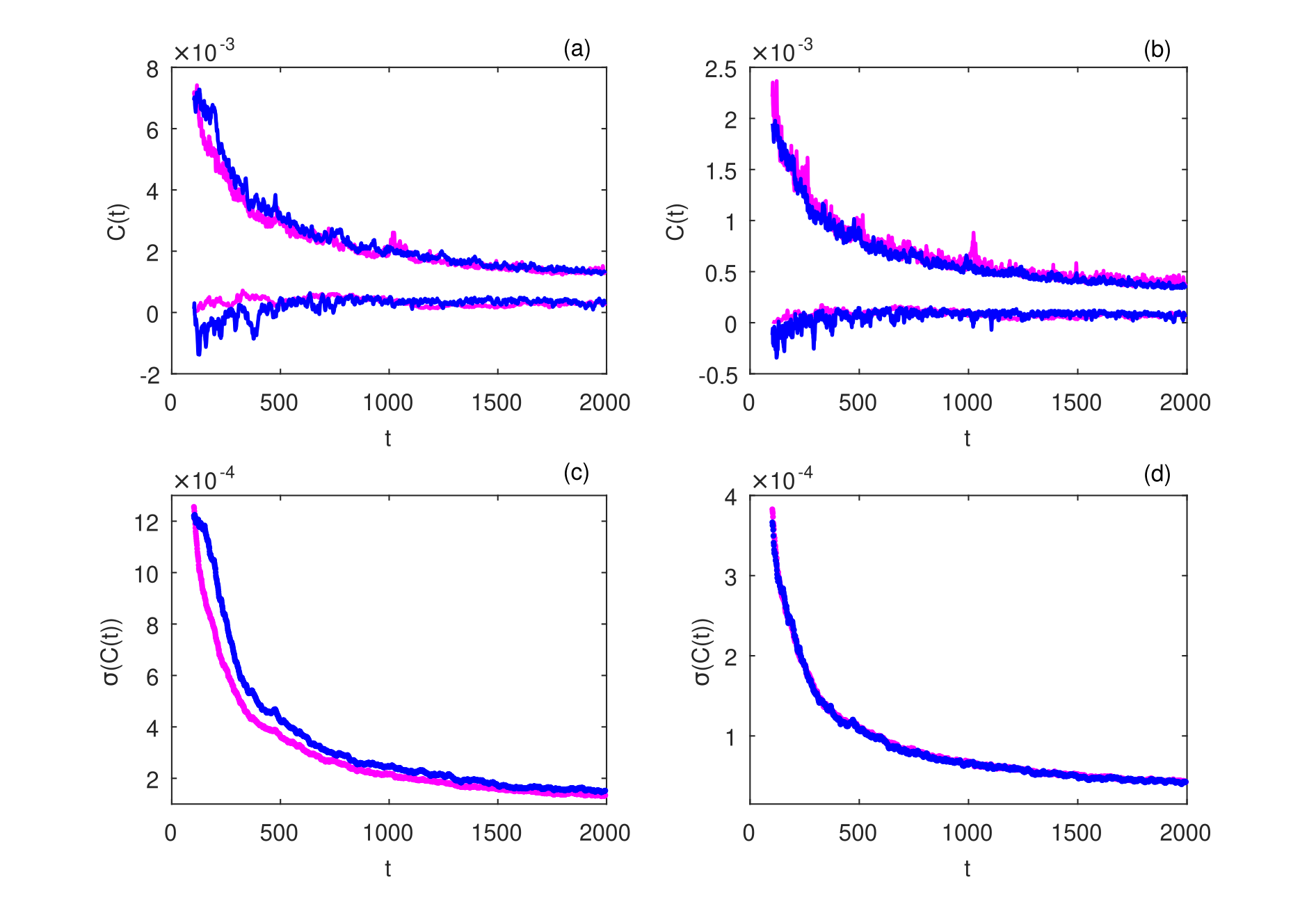
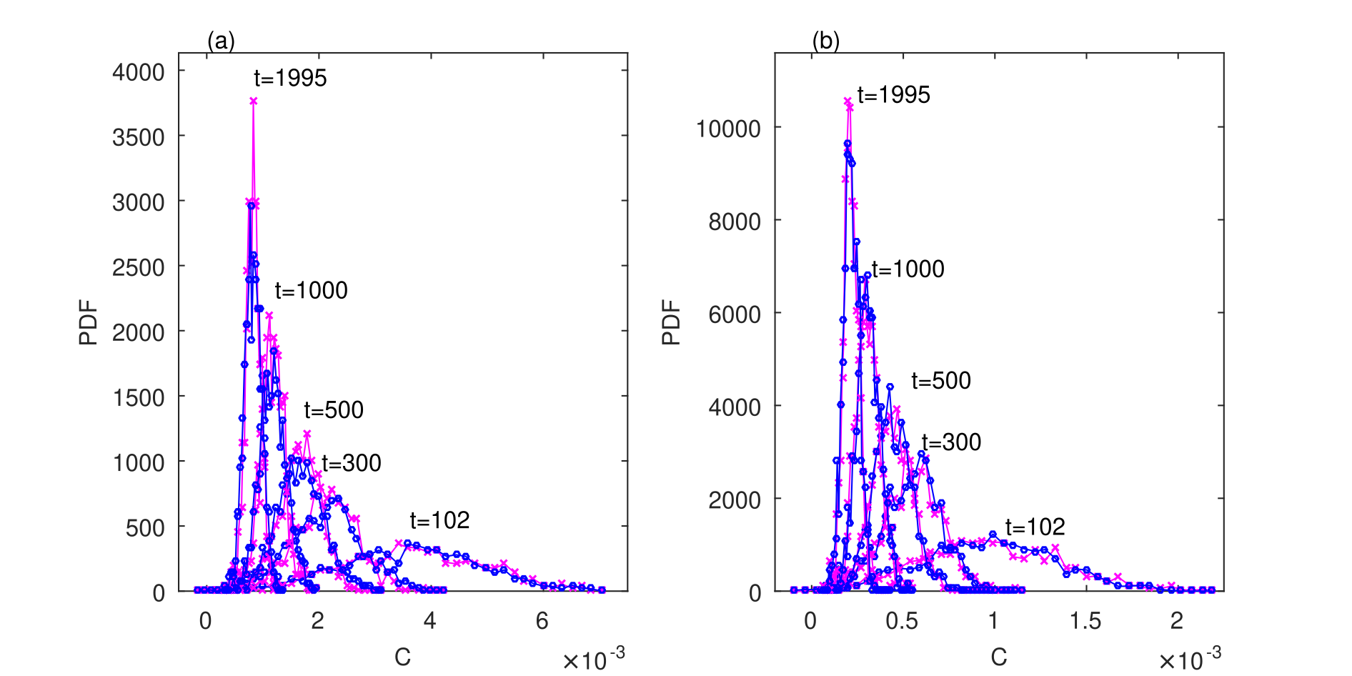
Since the numerical transition zone at the beginning of the time series takes longer, the model parameters can be determined only for times larger than . Fig. 1 shows that the extreme values and the standard deviations obtained from the time series models approximate the values obtained from the MC ensembles with lower accuracy than in case of cross-section sampling domain (see Fig. 6). In case of the smaller sampling domain of 1 m 1 m the approximation is better, because the fluctuations of the number of particles are smaller than when sampled in the larger domain of 2 m 2 m domain. The estimations of the concentration PDF shown in Fig 2 are still acceptable, being more accurate in case of the 1 m 1 m domain.
A.3 Influence of
To get a hint on the influence of increasing the variance of the field, we use an ensemble of time series obtained from MC-GRW simulations of non-reactive transport in Kraichnan velocity fields generated with , for the same initial condition, sampling time, and sampling domain as in case [37].
Though these fields are no longer acceptable first-order approximations of the Darcy flow velocity, they can be used to illustrate the effect of high velocity heterogeneity on the structure of the time series process. To avoid the effect of particle trapping which occurs at large times in two-dimensional simulations with particles in case of large velocity fluctuations [22], the length of the time series has been limited to days.
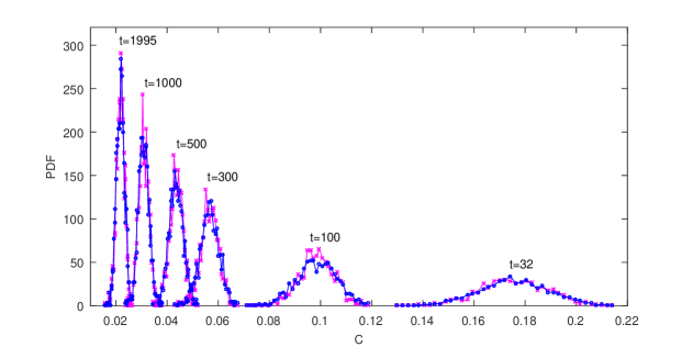
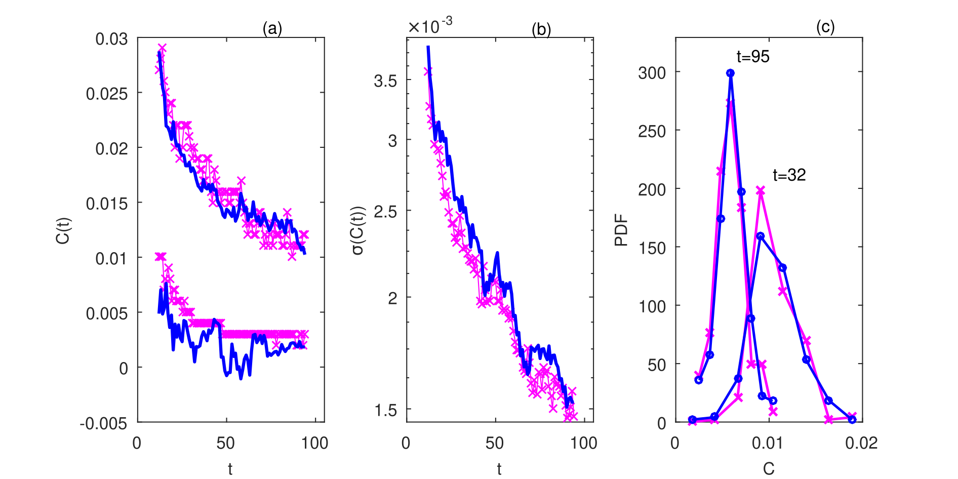
Repeating the analysis from Sections 3-5, we found that the time series process has the same structure as in case of small variability of the velocity field, with modified numerical parameters. The regression coefficient can be approximated by a power low, similarly to the case with small variance . Since larger velocity fluctuations enhance mixing, the smoothing of the discontinuous initial condition is faster than for small variability and the model is already valid for , where . The extreme values and the standard deviation of the ensemble of time series are reproduced with lower accuracy than in case (Figs. 3(a) and 3(b)) but the estimation of the concentration PDF is still satisfactory (Fig. 3(c)).
References
- [1] Geer FC, Kronvang B, Broers HP. High resolution monitoring of nutrients in groundwater and surface waters: process understanding, quantification of loads and concentrations and management applications. Hydrol Earth Syst Sci 2016;20:3619–3629. http://dx.doi.org/10.5194/hess-2016-169.
- [2] Turkeltaub T, Kurtzman D, Dahan O. Real-time monitoring of nitrate transport in the deep vadose zone under a crop field – implications for groundwater protection. Hydrol Earth Syst Sci 2016;20(8):3099–3108. http://dx.doi.org/10.5194/hess-20-3099-2016.
- [3] Meerschaert MM, Dogan M, Van Dam RL, Hyndman DW, Benson DA. Hydraulic conductivity fields: Gaussian or not?, Water Resour Res 2013; 49:4730–4737. http://dx.doi.org/10.1002/wrcr.20376.
- [4] Riva M, Neuman SP, Guadagnini A. New scaling model for variables and increments with heavy-tailed distributions. Water Resour Res 2015;51:4623–4634. http://dx.doi.org/10.1002/2015WR016998.
- [5] Mandelbrot B, Wallis JR. Noah, Joseph, and operational hydrology. Water Resour Res 1968;4(5):909–918. http://dx.doi.org/10.1029/WR004i005p00909.
- [6] Mandelbrot B, Wallis JR. Some long-run properties of geophysical records. Water Resour Res 1969;5(2):321–340. http://dx.doi.org/10.1029/WR005i002p00321.
- [7] Mandelbrot B, Van Ness JW. Fractional Brownian motions, fractional noises and applications. SIAM Rev 1968;10(4):422–437. http://dx.doi.org/10.1137/1010093.
- [8] Molz FJ, Liu HH, Szulga J. Fractional Brownian motion and fractional Gaussian noise in subsurface hydrology: A review, presentation of fundamental properties, and extensions. Water Resour Res 1997;33(10):2273–2286. http://dx.doi.org/10.1029/97WR01982.
- [9] Liu G, Butler Jr. JJ, Bohling GC, Reboulet E, Knobbe S, Hyndman DW. A new method for high-resolution characterization of hydraulic conductivity. Water Resour Res 2009;W08202. http://dx.doi.org/10.1029/2009WR008319.
- [10] Vamoş C, Crăciun M, Suciu N. Automatic algorithm to decompose discrete paths of fractional Brownian motion into self-similar intrinsic components, Eur Phys J B 2015;88:250. http://dx.doi.org/10.1140/epjb/e2015-60515-5.
- [11] Dentz M, Tartakovsky DM. Probability density functions for passive scalars dispersed in random velocity fields. Geophys Res Lett 2010;37:L24406. http://dx.doi.org/10.1029/2010GL045748.
- [12] Pope SB. PDF methods for turbulent reactive flows. Progr Energ Combust Sci 1985;11(2):119–192. http://dx.doi.org/10.1016/0360-1285(85)90002-4.
- [13] Pope SB. Turbulent Flows. Cambridge: Cambridge University Press: 2000.
- [14] Sanchez-Vila X, Guadagnini A, Fernàndez-Garcia D. Conditional probability density functions of concentrations for mixing-controlled reactive transport in heterogeneous aquifers. Math Geosci 2009;41:323–351. http://dx.doi.org/10.1007/s11004-008-9204-2.
- [15] Meyer DW, Jenny P, Tchelepi HA. A joint velocity-concentration PDF method for tracer flow in heterogeneous porous media. Water Resour Res 2010;46:W12522. http://dx.doi.org/10.1029/2010WR009450.
- [16] Suciu N, Radu FA, Attinger S, Schüler L, Knabner P. A Fokker-Planck approach for probability distributions of species concentrations transported in heterogeneous media. J Comput Appl Math 2015;289:241–252. http://dx.doi.org/10.1016/j.cam.2015.01.030.
- [17] Suciu, N, Schüler, L., Attinger, S, Knabner, P. Towards a filtered density function approach for reactive transport in groundwater. Adv Water Resour 2016;90:83–98. http://dx.doi.org/10.1016/j.advwatres.2016.02.016.
- [18] Vamoş C, Suciu N, Vereecken H. Generalized random walk algorithm for the numerical modeling of complex diffusion processes. J Comput Phys 2003;186(2):527–544. http://dx.doi.org/10.1016/S0021-9991(03)00073-1.
- [19] Brockwell PJ, Davis RA. Time Series: Theory and Methods. New York: Springer-Verlag: 1987.
- [20] Hamilton JD. Time series analysis. Princeton: Princeton University Press: 1994.
- [21] Landau LD, Lifshitz EM. Physique statistique. Moscou: Mir: 1984.
- [22] Suciu N, Vamoş C, Vanderborght J, Hardelauf H, Vereecken H. Numerical investigations on ergodicity of solute transport in heterogeneous aquifers. Water Resour Res 2006;42:W04409. http://dx.doi.org/10.1029/2005WR004546.
- [23] Suciu N, Vamos C, Radu FA, Vereecken H, Knabner P. Persistent memory of diffusing particles. Phys Rev E 2009;80:061134. http://dx.doi.org/10.1103/PhysRevE.80.061134.
- [24] Suciu N. Diffusion in random velocity fields with applications to contaminant transport in groundwater. Adv Water Resour 2014;69:114–133. http://dx.doi.org/10.1016/j.advwatres.2014.04.002.
- [25] Kraichnan RH. Diffusion by a random velocity field. Phys Fluids 1970;13(1):22–31. http://dx.doi.org/10.1063/1.1692799.
- [26] Andričević R. Effects of local dispersion and sampling volume on the evolution of concentration fluctuations in aquifers. Water Resour Res 1998;34(5):1115–1129. http://dx.doi.org/10.1029/98WR00260.
- [27] Fiori A, Dagan G. Concentration fluctuations in aquifer transport: A rigorous first-order solution and applications. J Contam Hydrol 2000;45(1):139–163. http://dx.doi.org/10.1016/S0169-7722(00)00123-6.
- [28] Caroni E, Fiorotto V. Analysis of concentration as sampled in natural aquifers. Transport in porous media 2005;59(1):19–45. http://dx.doi.org/10.1007/s11242-004-1119-x.
- [29] Schüler L, Suciu N, Knabner P, Attinger S. A time dependent mixing model to close PDF equations for transport in heterogeneous aquifers. Adv Water Resour 2016;96:55–67. http://dx.doi.org/10.1016/j.advwatres.2016.06.012.
- [30] Taylor SJ. Modelling financial time series (2nd edition). Singapore: World Scientific Publishing: 2007.
- [31] Bohm G, Zech G. Introduction to Statistics and Data Analysis for Physicists. Hamburg: Verlag Deutsches Elektronen-Synchrotron: 2010.
- [32] Vamoş C, Crăciun M. Automatic Trend Estimation. Dordrecht: Springer: 2012.
- [33] Kitagawa G, Gersch W. A smoothness priors time-varying AR coefficient modeling of nonstationary covariance time series. IEEE Trans Automat Contr 1985;30(1):48–56. http://dx.doi.org/10.1109/TAC.1985.1103788.
- [34] Moulines E, Priouret P, Roueff F. On recursive estimation for time varying autoregressive processes. Ann Stat 2005;33(6):2610–2654. http://dx.doi.org/10.1214/009053605000000624.
- [35] Mehta DD, Rudoy D and Wolfe PJ. Kalman-based autoregressive moving average modeling and inference for formant and antiformant tracking a. J Acoust Soc Am 2012;132(3):1732–1746. http://dx.doi.org/10.1121/1.4739462.
- [36] Demmy G, Berglund S, Graham W. Injection mode implications for solute transport in porous media: Analysis in a stochastic Lagrangian framework. Water resources research. 1999;35(7):1965-1973. http://dx.doi.org/10.1029/1999WR900027.
- [37] Suciu N, Vamos C, Vereecken H, Knabner P. Global random walk simulations for sensitivity and uncertainty analysis of passive transport models. Ann Acad Rom Sci Ser Math Appl 2011;3(1):218–234.
[1] R. Andričević, Effects of local dispersion and sampling volume on the evolution of concentration fluctuations in aquifers,Water Resour. Res., 34 (5) (1998), pp. 1115-1129
CrossRef (DOI)
[2] G. Bohm, G. Zech, Introduction to Statistics and Data Analysis for Physicists, Verlag Deutsches Elektronen-Synchrotron, Hamburg (2010)
[3] P.J. Brockwell, R. Davis, Time Series: Theory and Methods, Springer-Verlag, New York (1987)
[4] E. Caroni, V. Fiorotto, Analysis of concentration as sampled in natural aquifers, Transp. Porous Media, 59 (1) (2005), pp. 19-45
CrossRef (DOI)
[5] G. Demmy, S. Berglund, W. Graham, Injection mode implications for solute transport in porous media: analysis in a stochastic Lagrangian framework, Water Resour. Res., 35 (7) (1999), pp. 1965-1973
CrossRef (DOI)
[6] M. Dentz, D. Tartakovsky, Probability density functions for passive scalars dispersed in random velocity fields, Geophys. Res. Lett., 37 (2010), p. L24406
CrossRef (DOI)
[7] A. Fiori, G. Dagan, Concentration fluctuations in aquifer transport: a rigorous first-order solution and applications, J. Contam. Hydrol., 45 (1) (2000), pp. 139-163
CrossRef (DOI)
[8] F.C. Geer, B. Kronvang, H.P. Broers, High resolution monitoring of nutrients in groundwater and surface waters: process understanding. Quantification of loads and concentrations and management applications, Hydrol. Earth Syst. Sci., 20 (2016), pp. 3619-3629
CrossRef (DOI)
[9] J. Hamilton, Time Series Analysis, Princeton University Press, Princeton (1994)
[10] G. Kitagawa, W. Gersch, A smoothness priors time-varying AR coefficient modeling of nonstationary covariance time series, IEEE Trans. Autom. Control, 30 (1) (1985), pp. 48-56
CrossRef (DOI)
[11] R. Kraichnan, Diffusion by a random velocity field, Phys. Fluids, 13 (1) (1970), pp. 22-31
CrossRef (DOI)
[12] L.D. Landau, E. Lifshitz, Physique Statistique, Mir, Moscou (1984)
[13] G. Liu, J.J.J. Butler, G.C. Bohling, E. Reboulet, S.Knobbe, D. Hyndman, A new method for high-resolution characterization of hydraulic conductivity, Water Resour. Res (2009)
CrossRef (DOI)
[14] B. Mandelbrot, J.R. Wallis, Noah, Joseph, and operational hydrology, Water Resour. Res., 4 (5) (1968), pp. 909-918
CrossRef (DOI)
[15] B. Mandelbrot, J. Van Ness, Fractional Brownian motions, fractional noises and applications, SIAM Rev., 10 (4) (1968), pp. 422-437
CrossRef (DOI)
[16] B. Mandelbrot, J.R. Wallis, Some long-run properties of geophysical records, Water Resour. Res., 5 (2) (1969), pp. 321-340
CrossRef (DOI)
[17] M.M. Meerschaert, M. Dogan, R.L. Van Dam, D.W.Hyndman, D. Benson, Hydraulic conductivity fields: Gaussian or not?, Water Resour. Res., 49 (2013), pp. 4730-4737
CrossRef (DOI)
[18] D.D. Mehta, D. Rudoy, P. Wolfe, Kalman-based autoregressive moving average modeling and inference for formant and antiformant tracking a, J. Acoust. Soc. Am., 132 (3) (2012), pp. 1732-1746
CrossRef (DOI)
[19] D.W. Meyer, P. Jenny, H. Tchelepi, A joint velocity-concentration PDF method for tracer flow in heterogeneous porous media, Water Resour. Res., 46 (2010), p. W12522
CrossRef (DOI)
[20] F.J. Molz, H.H. Liu, J. Szulga, Fractional Brownian motion and fractional gaussian noise in subsurface hydrology: a review, presentation of fundamental properties, and extensions, Water Resour. Res., 33 (10) (1997), pp. 2273-2286
CrossRef (DOI)
[21] E. Moulines, P. Priouret, F. Roueff, On recursive estimation for time varying autoregressive processes, Ann. Stat., 33 (6) (2005), pp. 2610-2654
CrossRef (DOI)
[22] S. Pope, PDF Methods for turbulent reactive flows, Prog. Energy Combust. Sci., 11 (2) (1985), pp. 119-192
CrossRef (DOI)
[23] S. Pope, Turbulent Flows, Cambridge University Press, Cambridge (2000)
[24] M. Riva, S.P. Neuman, A. Guadagnini, New scaling model for variables and increments with heavy-tailed distributions, Water Resour. Res., 51 (2015), pp. 4623-4634
CrossRef (DOI)
[25] X. Sanchez-Vila, A. Guadagnini, D. Fernàndez-Garcia, Conditional probability density functions of concentrations for mixing-controlled reactive transport in heterogeneous aquifers, Math. Geosci., 41 (2009), pp. 323-351
CrossRef (DOI)
[26] L. Schüler, N. Suciu, P. Knabner, S. Attinger, A time dependent mixing model to close PDF equations for transport in heterogeneous aquifers, Adv. Water Resour., 96 (2016), pp. 55-67
CrossRef (DOI)
[27] N. Suciu, Diffusion in random velocity fields with applications to contaminant transport in groundwater, Adv. Water Resour., 69 (2014), pp. 114-133
CrossRef (DOI)
[28] N. Suciu, F.A. Radu, S. Attinger, L. Schüler, P. Knabner, A Fokker-Planck approach for probability distributions of species concentrations transported in heterogeneous media, J. Comput. Appl. Math., 289 (2015), pp. 241-252
CrossRef (DOI)
[29] N. Suciu, L. Schüler, S. Attinger, P. Knabner, Towards a filtered density function approach for reactive transport in groundwater, Adv. Water Resour., 90 (2016), pp. 83-98
CrossRef (DOI)
[30] N. Suciu, C. Vamoş, J. Vanderborght, H. Hardelauf, H.Vereecken, Numerical investigations on ergodicity of solute transport in heterogeneous aquifers, Water Resour. Res., 42 (2006), p. W04409
CrossRef (DOI)
[31] N. Suciu, C. Vamoş, F.A. Radu, H. Vereecken, P. Knabner, Persistent memory of diffusing particles, Phys. Rev. E, 80 (2009), p. 061134
CrossRef (DOI)
[32] N. Suciu, C. Vamos, H. Vereecken, P. Knabner, Global random walk simulations for sensitivity and uncertainty analysis of passive transport models, Ann. Acad. Rom. Sci. Ser. Math. Appl., 3 (1) (2011), pp. 218-234
(article on the journal website)
[33] S. Taylor, Modelling Financial Time Series (2nd ed.), World Scientific Publishing, Singapore (2007)
[34] T. Turkeltaub, D. Kurtzman, O. Dahan, Real-time monitoring of nitrate transport in the deep vadose zone under a crop field – implications for groundwater protection, Hydrol. Earth Syst. Sci., 20 (8) (2016), pp. 3099-3108
CrossRef (DOI)
[35] C. Vamoş, M. Crăciun, Automatic Trend Estimation, Springer, Dordrecht (2012)
CrossRef (DOI)
[36] C. Vamoş, M. Crăciun, N. Suciu, Automatic algorithm to decompose discrete paths of fractional Brownian motion into self-similar intrinsic components, Eur. Phys. J. B, 88 (2015), p. 250
CrossRef (DOI)
[37] C. Vamoş, N. Suciu, H. Vereecken, Generalized random walk algorithm for the numerical modeling of complex diffusion processes, J. Comput. Phys., 186 (2) (2003), pp. 527-544
CrossRef (DOI)