Abstract
Fractional Brownian motion (fBm) is a nonstationary self-similar continuous stochastic process used to model many natural phenomena. A realization of the fBm can be numerically approximated by discrete paths which do not entirely preserve the self-similarity. We investigate the self-similarity at different time scales by decomposing the discrete paths of fBm into intrinsic components. The decomposition is realized by an automatic numerical algorithm based on successive smoothings stopped when the maximum monotonic variation of the averaged time series is reached. The spectral properties of the intrinsic components are analyzed through the monotony spectrum defined as the graph of the amplitudes of the monotonic segments with respect to their lengths (characteristic times). We show that, at intermediate time scales, the mean amplitude of the intrinsic components of discrete fBms scales with the mean characteristic time as a power law identical to that of the corresponding continuous fBm. As an application we consider hydrological time series of the transverse component of the transport process generated as a superposition of diffusive movements on advective transport in random velocity fields. We found that the transverse component has a rich structure of scales, which is not revealed by the analysis of the global variance, and that its intrinsic components may be self-similar only in particular cases.
Authors
Keywords
Computational Methods; time series analysis; intrinsic components; groundwater
Cite this paper as:
C. Vamoş, M. Crăciun, N. Suciu, Automatic algorithm to decompose discrete paths of fractional Brownian motion into self-similar intrinsic components, Eur. Phys. J. B (2015) 88: 250.
doi: 10.1140/epjb/e2015-60515-5
References
About this paper
Journal
The European Physical Journal B
Publisher Name
Springer Berlin Heidelberg
Print ISSN
1434-6028
Online ISSN
1434-6036
Automatic algorithm to decompose discrete paths of fractional Brownian motion into self-similar intrinsic components
- 1 “T. Popoviciu” Institute of Numerical Analysis, Romanian Academy, P.O. Box 68, 400110 Cluj-Napoca, Romania
- 2 Mathematics Department, Friedrich Alexander University of Erlangen-Nuremberg, Cauerstraße 11, 91058 Erlangen, Germany
Abstract
Fractional Brownian motion (fBm) is a nonstationary self-similar continuous stochastic process used to model many natural phenomena. A realization of the fBm can be numerically approximated by discrete paths which do not entirely preserve the self-similarity. We investigate the self-similarity at different time scales by decomposing the discrete paths of fBm into intrinsic components. The decomposition is realized by an automatic numerical algorithm based on successive smoothings stopped when the maximum monotonic variation of the averaged time series is reached. The spectral properties of the intrinsic components are analyzed through the monotony spectrum defined as the graph of the amplitudes of the monotonic segments with respect to their lengths (characteristic times). We show that, at intermediate time scales, the mean amplitude of the intrinsic components of discrete fBms scales with the mean characteristic time as a power law identical to that of the corresponding continuous fBm. As an application we consider hydrological time series of the transverse component of the transport process generated as a superposition of diffusive movements on advective transport in random velocity fields. We found that the transverse component has a rich structure of scales, which is not revealed by the analysis of the global variance, and that its intrinsic components may be self-similar only in particular cases.
PACS:
- 05.40.Jc — Brownian motion
- 05.45.Tp — Time series analysis
- 92.40.Kf — Groundwater
1 Introduction
Complex multiscale nonlinear and nonstationary time series need special algorithms to identify, separate, and analyze their evolution at different scales gao2007 . Traditional data analysis methods, including the multiresolution analysis supplied by the wavelet decomposition percival2000 , are not well suited for such a task because they are based on pre-determined basis and have a nonadaptive character. An alternative is the empirical mode decomposition (EMD) method, a data-driven numerical algorithm which decomposes a time series into several intrinsic spectral components arranged in a hierarchy of time scales huang98 . The EMD method was recently extended to more efficient and mathematically rigorous algorithms: the iterative filtering lin2009 , the synchrosqueezed wavelet transform daubech2011 , and the sparse time-frequency representation hou2011 .
A critical problem for any time series decomposition into a hierarchy of spectral components is the manner in which the time scale is defined. In the case of the classical Fourier analysis one uses the frequency of the constant amplitude trigonometric components which is a global quantity that can be generalized only for periodic components. The EMD and its subsequent modifications use the instantaneous frequency of signals, but this notion is controversial in mathematics and engineering boasas1992 .
An alternative and more general approach to the time scale issue is provided by the characteristic times defined as the spacings between successive local extrema of time series, also equal to the lengths of their monotonic segments huang98 . Hence the time series is decomposed into a sequence of monotonic segments and the analysis is focused on the monotony properties of the time series. Instead of the usual power spectrum we introduce the monotony spectrum of the time series obtained by plotting the amplitudes of the monotonic segments as a function of their duration (the characteristic times) vamos2014 .
In the case of a noisy time series, the noise fluctuations hide the variations of the larger scale components and the monotony spectrum contains information only on the variations of the smallest time scales. The variations of larger scales separated from those of small scales are available through the intrinsic components of a spectral decomposition of the time series. That is why a complete description of a time series is obtained only by the monotony spectra of all the intrinsic components. We obtained such a description for the returns of several financial indices after we decomposed them into disjoint multiplicative intrinsic components vamos2014 . In this paper we continue this approach in order to obtain additive decompositions of self-similar non-stationary time series without imposing the disjoint condition.
A simple method to eliminate the small scale fluctuations is the smoothing by successive moving averages (MA). The main difficulty to find an intrinsic component by repeated MAs is to establish a rigorous criterion to stop the averagings so that the resulting component preserve the essential properties of the initial time series. For instance, in iterative filtering this criterion consists of imposing an artificial threshold for the difference between the initial time series and the sum of the components already determined lin2009 . The novelty of our algorithm is given by a simple criterion, without any parameter, based on the determination of the maximum monotonic variation during the repeated MAs. This parameter-free criterion allows us to design an automatic algorithm to decompose some types of time series into intrinsic components.
We verify the decomposition algorithm by applying it on discrete paths of fractional Brownian motion (fBm) which have well-known self-similarity properties mandel1968 . We show that the intrinsic components that we obtain preserve the basic self-similarity of fBm. Furthermore, the range of time scales for which the self-similarity is satisfied increases with the length of the finite fBm and the largest and the smallest scales are not self-similar. The discrete fBms shorter than 500 values do not have self-similar intrinsic components. The ability of moving averages to make obvious the self-similarity of fBm has also been proved for the segments limited by the intersections between the fBm path and its smoothed form carbone2004 ; carbone2007 .
Our new algorithm decomposes the time series containing a hierarchy of time scales with the amplitude decreasing monotonically from the large scales to the small scales, as for example the discrete fBm, but it cannot decompose time series if the variations with the largest amplitudes occur at the smallest time scales. Even with this limitation, our algorithm has many possible applications. For example fBm is used in modelling phenomena in hydrology mandel1968b ; graves2014 ; suciu2010 , finance shiryaev1999 ; cont2005 , network traffic leland1994 ; stoev2005 , geophysics turcotte1997 and many other domains addison1997 .
In stochastic subsurface hydrology, the fBm may be used as a model for the trajectory of the transport process whenever the velocity field has long range power law correlations suciu2010 as well as a model of the preasymptotic regime in case of short-range correlation Trefryetal2003 ; Fiorietal2006 . In this article, as an application, we analyze hydrological time series of the transverse component of the transport process generated as a superposition of diffusive movements on advective transport in random velocity fields. The analysis of the corresponding time series with our automatic algorithm reveals that, in general, the transverse component of the transport process does not have intrinsic components obeying a self-similarity law. The results show a more complex structure of scales which cannot be detected by analytical or numerical estimations of the global variance.
2 Monotony spectrum
For an arbitrary time series we denote by , , the positions of the local extrema with the convention and . Therefore the time series has monotonic segments, the characteristic times are , and is the amplitude of the variation of the -th monotonic segment. In the simplest cases, the set supplies a full description of the time scales contained by the time series. For instance, a harmonic oscillation has all equal to half of the oscillation period. The situation is more complex in the case of a noisy time series. Then the characteristic times distribution is dominated by the small-scale fluctuations of the noise and it does not distinguish the large-scale variations possibly existing in the time series. Quantitatively, a time series cannot contain monotonic variations smaller than , but there may exist components with monotonic variations lasting longer than .
We exemplify this behavior of the characteristic times by means of an artificial time series numerically generated by the method described in vamos2008 ; vamos2012 . We construct a nonmonotonic trend from monotonic semiperiods of sinusoid with random amplitudes joined together such that the trend is continuous. The amplitudes of the sinusoids are random numbers with a uniform probability distribution. The trend is characterized by three parameters: the length of the time series , the number of monotonic segments , and the minimum number of points in a monotonic segment . These trends have a large variability homogeneously distributed throughout the entire definition interval. We superpose a white Gaussian noise over this trend. An additional parameter characterizes the ratio of the amplitude of the trend variations to that of the noise fluctuations. Figure 1a shows such an artificial time series with , , and .
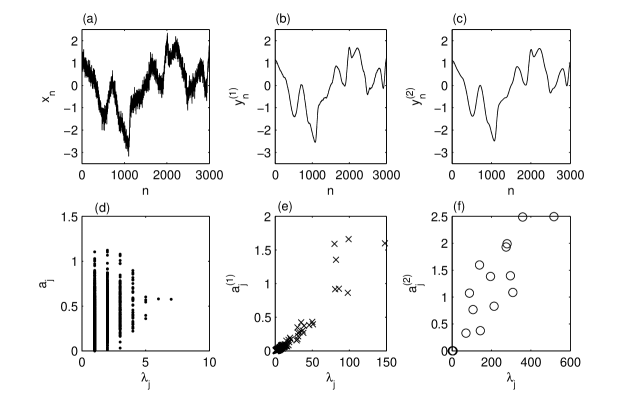
A detailed description of the monotonic segments is given by the monotony spectrum obtained by plotting the amplitudes with respect to characteristic times . In the monotony spectrum of the time series in Fig. 1a all the characteristic times are smaller than (Fig. 1d). The monotonic variations of hundreds of time steps of the trend do not appear in the monotony spectrum. As a result the monotony spectrum of the noisy time series is almost identical with that of the same noise without the trend (not presented here).
In order to determine the large scale variations we eliminate small scales using the smoothing with the repeated central moving average vamos2012 . We consider a succession of averagings and we denote the time series averaged times by with the convention . The -th moving average is defined as
| (1) |
where is the semilength of the averaging window and . If (), then the average is taken over the first (the last ) values of . The properties of this moving average are analyzed in vamos2012 .
The time series obtained after a single and two successive averagings with of the time series in Fig. 1a are plotted in Figs. 1b and 1c and the corresponding monotony spectra in Figs. 1e and 1f. After the first averaging the most of the small scale fluctuations are eliminated, nevertheless the largest scale variations are interrupted by small residual inflections (Fig. 1b). The monotony spectrum contains seven monotonic segments longer than 50 time steps and many fluctuations with smaller scales (Fig. 1e). After the second averaging, only five fluctuations shorter than 5 time steps remain and almost all the monotonic segments of the trend are present in (Fig. 1f). The variation of the monotony spectrum illustrates the well-known numerical method to estimate the trend by smoothing the short scale fluctuations.
3 Maximum monotonic variation
A critical issue related to the trend extraction by repeated averagings is the stopping criterion. If the averagings are stopped too soon then the noise fluctuations are not eliminated; on the other hand if they are stopped too late, then the fluctuations are smoothed out but the trend could be distorted by oversmoothing vamos2012 . We present here a stopping criterion which has no parameters and is based on the monotony properties of the time series.
We consider successive averagings with given and we denote by the maximum amplitude of the monotonic variations of time series averaged times and we denote by
| (2) |
the maximum amplitude of all the monotonic segments occurring until the -th averaging. From this definition it follows that is monotonically increasing. We denote by its maximum value to which it asymptotically tends and which is the maximum monotonic variation of a time series. In fact is reached in a finite number of averagings and after that remains constant. This behavior results from the fact that tends to zero when , so that it has to exist a maximum corresponding to the average.
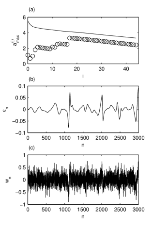
The optimum smoothing of the time series is that given by the averaging because all the monotonic variations of the next averagings are smaller than . Hence we have to determine , but the variation of with respect to is not monotonic and it can have many local maxima (see for instance Fig. 2a). The value of can take different values depending on the relation between the amplitudes of the small scale fluctuations and those of the large scale variations and also on their smoothing rates. Therefore it is difficult to establish whether the maximum obtained after a certain number of averagings is the real one or whether a larger one could be obtained during the next averagings.
In order to design a stopping criterion, without any subjective implication, we use the global variation of the time series averaged times
is strictly decreasing with respect to the number of averagings and it tends asymptotically to zero. The equality is possible only if there exist more than successive values equal to the global maximum and others equal to the global minimum. We do not consider such special time series in our study.
We have the obvious relation ; the equality takes place when the two global extrema are the ends of the same monotonic segment. We denote by the smallest value of the index for which . Then for every we have the inequalities
| (3) |
meaning that in Eq. (2), which is monotonically increasing, cannot be larger than , so that . As a general rule and then is constant for . The smoothings are stopped after averagings when for the first time the inequality holds and we can determine also which corresponds to the maximum monotonic variation.
We apply the maximum monotonic variation criterion to the time series analyzed in the previous section (Fig. 1a). The stopping condition of the averagings is fulfilled after averagings and the maximum monotonic variation occurs for (Fig. 2a). As discussed above, has a monotonic variation (continuous line), whereas has several maxima and minima until it reaches the global maximum (circle markers). The time series averaged times approximates very well the trend, the absolute values of the local relative error being smaller than 0.08 (Fig. 2b). Its absolute values are greater than 0.03 only where the trend has large slopes. In these regions the residuals have fluctuations with larger amplitudes than in other regions (Fig. 2c). Due to these distortions is uncorrelated (white) only for lags larger than 22 time steps, but it is Gaussian with a very good approximation (the Kolmogorov-Smirnov index is 0.013).
We have thus shown that the maximum monotonic variation criterion provides a correct decomposition of the analyzed time series which has the time scales concentrated in two disjoint intervals: the deterministic trend corresponds to the large scales and the Gaussian white noise to the small scales (Fig. 3). But if the amplitudes of the noise fluctuations are much larger than those of the trend variations, then the decomposition does not work. Indeed, the separation of the components of different scales is possible only if the successive averagings smooth faster the small scale variations than those of large scale. Although the noise attenuation rate is larger due to its fast sign variations, if the noise amplitude is very large, then it is possible that the trend is damped first and the large scale component cannot be extracted.
A special case is that of the time series containing a hierarchy of time scales dominated by the large ones. Such time series are the discrete paths of fBm. In the following we describe an automatic algorithm to extract a hierarchy of components from a discrete fBm using the maximum monotonic variation criterion. Since the algorithm uses no parameter, these components are intrinsic, completely determined by the available data.
We introduce a distinct notation for the intrinsic components successively extracted. If is the total number of intrinsic components, then the -th intrinsic component is , . It is obtained by applying the maximum monotonic variation algorithm to the residuals , while the next residuals are equal to . The order one residuals are identical with the initial time series .
First we choose the semilengths of the averaging windows such that we gradually increase the smoothing. When the monotony spectrum is plotted for the initial time series. The intrinsic component that we search is given by . The extraction of the intrinsic components stops when the algorithm does not succeed to extract a new intrinsic component. This happens if , i.e., the maximum monotonic variation occurs for the unsmoothed residuals.
4 Intrinsic components of fBm
The fractional Brownian motion (fBm) was defined as a moving average of the past increments of an ordinary Brownian motion by means of a power type smoothing kernel mandel1968 . The exponent of the fBm process is related to its self-similarity property, i.e., the processes and have the same probability distribution. The fBm is nonstationary with the variance varying in time as a power law . In fact the fBm is the single Gaussian stochastic process with stationary increments, continuous mean square and satisfying the self-similarity property mandel1968 . When , the fBm reduces to ordinary Brownian motion.
The fBm is a continuous stochastic process and there are many numerical algorithms to generate its discrete paths bardet2003 . We use the algorithm based on the wavelet decomposition meyer2000 which is an improved form of that designed in abrysellan1996 . It provides a good approximation of the fBm path if is not close to 0.1. Obviously, by discretization some of the self-similarity properties of the fBm are lost. Our decomposition into intrinsic components allows us to show that the self-similarity is distorted for the smallest and largest time scales.
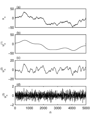
We apply the algorithm described in the previous section to a discrete fBm with and (Fig. 4a). Three intrinsic components are obtained (Figs. 4b-d), the last of them is Gaussian (the Kolmogorov-Smirnov index is 0.011) and uncorrelated except for a lag equal to one time step. The global variations of the three components are: , , and . Hence the analyzed time series is dominated by large time scales and, because , the amplitudes of the monotonic variations decrease rapidly as the time scale decreases.
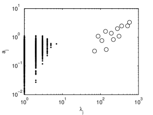
The monotony spectra of the three intrinsic components are plotted in log-log scale in Fig. 5. Although the number of the monotonic segments varies strongly (, , and ), their monotony spectra do not superpose and have similar shapes. However, only the monotony spectrum of the second intrinsic component has a well-defined shape while that of the first intrinsic component has too few points and that of the third intrinsic component is distorted because the monotonic segments have the minimum length limited by the time step. The elongated shape of the monotony spectra shows that the amplitudes of the monotonic segments in each intrinsic component increase with the increase of their characteristic times. Since we use a log-log plot, this dependence indicates the existence of a power law.
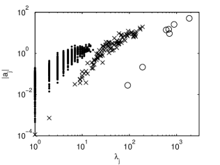
If the intrinsic components are correctly determined, then their structure has to reflect in some way the self-similarity law of the fBm. We notice that the mean amplitudes of the monotony spectra of the intrinsic components in Fig. 5 decrease with the decrease of the mean characteristic times. We investigate this behavior on a statistical ensemble of 100 discrete fBms with and with a fixed value of . For each intrinsic component of each fBm path we compute the mean of the characteristic times and the mean of the amplitudes of the monotonic segments. Then the coordinates give the center of mass of a monotony spectrum of the intrinsic component in linear coordinates.
The results for two statistic ensembles of 100 discrete fBms with and are plotted in log-log coordinates in Fig. 6. Before verifying the existence of the power law, we notice that at small and large values of in Fig. 6 the centers of mass of the intrinsic components arrange themselves on distinct line segments. The two alignments have different causes.
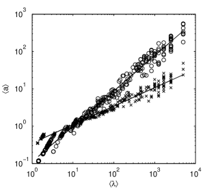
First we discuss the case of large time scales. The number of the monotonic segments of the intrinsic component is an integer, so that the mean characteristic time of a component takes only the discrete values . The maximum value is obtained if the intrinsic component is monotonic (). The next value occurs when and the distance in log-log coordinates between these two mean characteristic times is . When increases, these distances decrease. For large values of the values of are separated by intervals so small that they cannot be perceived separately on the graph.
The other alignment of the centers of mass at small is due to the discrete variations of the averaging window in Eq. (1). For small values of these jumps are perceptible and the centers of mass separate from each other. These discrete variations could be eliminated using a smooth averaging kernel, but the results are not essentially changed by such a procedure.
The centers of mass of the intrinsic components in log-log coordinates are distributed along two straight lines with slopes equal to and , values that approximate very well the Hurst parameters of the two statistical ensembles (Fig. 6). This result shows that the intrinsic components obtained with the maximum monotonic variation algorithm preserve the self-similarity property of fBm in the form
| (4) |
However, the distribution of the centers of mass about the regression lines is not homogeneous (Fig. 6). Due to the limited length of the time series the self-similarity does not hold at small scales near the time step or at large scales near the length of the time series. In the following we determine the interval of time scales on which the discrete paths of the fBm satisfy as close as possible the self-similarity law.
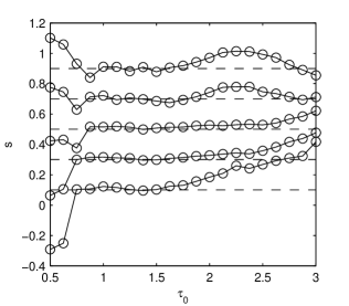
We denote by the order of magnitude of . We fit a straight line on the centers of mass for which is contained in the interval of unit length with the center on a fixed value . The slopes of these straight lines for different and for several values of are plotted in Fig. 7 for statistical ensembles with 1000 time series. A good approximation of is obtained in all cases for . Taking into account the unit width of the fitting interval, we can say that the centers of mass of the intrinsic components of fBm transform themselves into each other according to the self-similarity law (4) for , i.e., for two orders of magnitude. The intrinsic components with the center of mass outside of this interval (those with small and large time scales) do not obey the self-similarity law.
The length of the interval over which the self-similarity holds varies with the length of time series. We analyze this dependence using several statistical ensembles of 1000 time series with fixed and variable time series lengths . The orders of magnitude of the characteristic times for which the slope approximates with a relative error smaller than 0.03 are plotted in Fig. 8. The analysis has been made for two values of the Hurst parameter and . The interval for which the center of mass of the intrinsic components satisfies the self-similarity law increases with and for there are no self-similar intermediate scales.
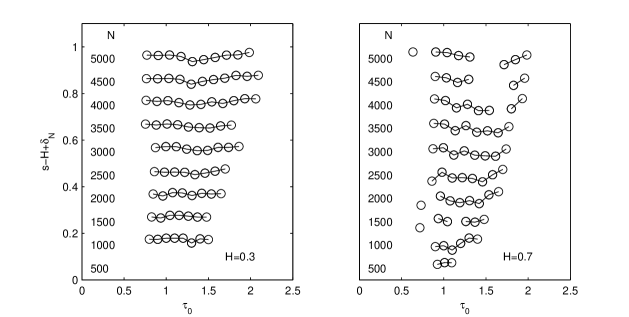
In Fig. 8, we notice that the centers of mass of the intrinsic components have large fluctuations for . It is likely that the numerical generation of discrete paths of fBm is weaker for large . One can use other numerical algorithms to obtain better paths. However, a comparison of different generation algorithms is beyond the scope of this article.
5 Intrinsic components of hydrological time series
In stochastic subsurface hydrology, the fBm naturally occurs as a model for the trajectory of the transport process whenever the velocity field has long range power law correlations suciu2010 . For short range correlations instead, the transport can be described asymptotically as a Gaussian diffusion Suciu2014 . However, for typical groundwater formations, the process converges to this Gaussian limit after long travel distances of hundreds of correlation lengths Trefryetal2003 so that the pre-asymptotic regime shows anomalous diffusion features Fiorietal2006 . While anomalous behavior in the pre-asymptotic regime of the longitudinal component of the transport process has been well documented Trefryetal2003 ; Fiorietal2006 , much less is known about the behavior of the transverse component.
As in the case of fBm, using the maximum monotonic variation algorithm, we analyze the time series describing the transverse component of the transport process generated by a popular numerical algorithm. We consider a typical model of the hydraulic conductivity for saturated aquifers consisting of a two-dimensional statistically homogeneous space random function, with exponential correlation of correlation length and variance Suciu2014 ; Schwarzeetal2001 . Realizations of this random function are generated by the well known Kraichnan algorithm Kraichnan1970 as sums of random periodic modes. The velocity samples are approximated, through a linearization of Darcy and continuity equations, by a slightly modified Kraichnan algorithm, as sum between a constant mean , with m/day, and a fluctuation given by a superposition of random periodic modes (Schwarzeetal2001, , Eq. 21). To avoid artificial un-physical fluctuations Eberhardetal2007 , the number of periodic modes is chosen of the order of the length of the time series to be generated.
We also consider an isotropic Gaussian diffusion process specified by a coefficient m2/day. The trajectory of the resulting advection-diffusion process is governed by a system of two Itô equations. Their solution is approximated by a weak Euler scheme Suciu2014 . Here we consider only the time series of the transverse trajectory component, less investigated in the past. The weak Euler approximation of the solution for the transverse trajectory component is given by
| (5) |
where , days is the time step, , is the solution for the longitudinal component, and is an unbiased random walk of amplitude Suciu2014 .
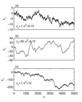
For fixed and , the properties of the time series (5) are controlled by the parameters and . For the present simulations we have chosen the ranges m m and . Figure 9 shows time series samples with for three extreme values of the parameters. The time series for the minimum values of and is plotted in Fig. 9a. Increasing to its maximum value leads to a time series dominated by large scale variations, the fluctuations being negligible (Fig. 9b). The fluctuations are also reduced when is increased, but less than in the previous case (Fig. 9c). The numerical generation algorithm for the chosen value of does not work when both of the two parameters take their maximum values.
Self-similarity properties of the hydrological time series are analyzed by the automatic algorithm used for discrete fBm in the previous section. In Figs. 10a-c we plot the results obtained for statistical ensembles of 1000 time series of length . One remarks that only for m and (Fig. 10c) the mean amplitudes are aligned along a straight line for all characteristic times, indicating the self-similarity property. When is set to its minimum value the linear alignment disappears, hence in this case the mean amplitudes of the intrinsic components do not satisfy a power law.
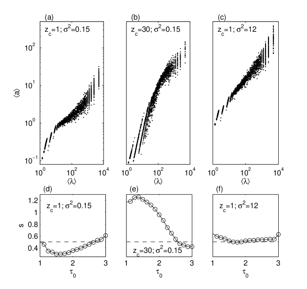
Even if the hydrological time series do not have a global self-similarity law, we can fit a straight line on the centers of mass of the intrinsic components as we have made in Fig. 6. In Fig. 10a the slope is indicating a normal diffusion. Increasing the value of is equivalent to expand the dimensionless time , so that time series with time steps correspond to the pre-asymptotic regime. This scale transformation explains why the shape of the graph in Fig. 10b is similar to the first part of the graph in Fig. 10a.
The global slope for Fig. 10b is indicating a super-diffusive behavior. These results are consistent with the behavior of the transverse diffusion coefficient obtained from Monte Carlo simulations with and , which increases to a maximum at about , followed by an asymptotic decay towards a constant value Suciu2014 ; Suciuetal2015b . Moreover, the variance of fits well with an fBm variance proportional to , with , from zero to the total simulation time , and with , from zero to . The transition between super-diffusion and diffusion passes through a sub-diffusive regime with , between and . We also found that the separation of these regimes, shown by differences between the corresponding Hurst coefficients, becomes even more pronounced as the correlation length increases from to Suciuetal2015b .
In the case shown in Fig. 10c, when the hydrological time series are self-similar, the global slope is , corresponding to a slightly super-diffusive behavior. Although the value is beyond the range of validity of the linear approximation of the velocity field, it provides an indication that the transverse transport may be super-diffusive only for extremely large spatial heterogeneity of the hydraulic conductivity. This is in qualitative agreement with numerical investigations on longitudinal transport which show that the anomalous behavior is mainly favored by the increase of Trefryetal2003 ; Fiorietal2006 .
A more detailed description of the hydrological time series is given by the variation of the slope computed for unit-length intervals of (Figs. 10d-f). If the slopes at the small time scales depend strongly on the parameter . For the minimum value of the slope is smaller than 0.5 for time scales with (Fig. 10d), indicating a sub-diffusive transport although the global behavior is diffusive. When m the slope is larger than 0.5 over the same range for (Fig. 10e); it can be even larger than 1, although for fBm . This super-diffusive behavior is in accordance with the global behavior in this case. For the largest value of considered in our simulations (Fig. 10f) the slope varies slightly between 0.5 and 0.6, in accordance with a global super-diffusive behavior.
The variation of the slope with the order of magnitude of the time scales for small variances , revealed by our decomposition method, corresponds qualitatively to the variation of the Hurst coefficient with the scale of observation inferred from Monte Carlo simulations Suciu2014 ; Suciuetal2015b (described above). However, an important difference should be noted here. Unlike the time scale used in our time series analysis, in numerical and experimental hydrological studies the scale is simply given by the time interval of the observation. As this interval increases, it encompasses more and more monotony intervals of length of the trajectory which contribute to its global variance. The power of the new decomposition method is that it considers the contribution of all the monotony scales of a time series from the beginning of the analysis, not gradually as in hydrological Monte Carlo approaches. The advantage in analyzing the diffusive behavior of the hydrodynamic time series is that it provides precisely identified and quantified contributions of the separated time scales, which are related to characteristic intervals of variation of the random velocity.
6 Conclusions
In this paper we analyze the spectral properties of nonlinear and nonstationary time series using the characteristic time equal with the distance between two successive local extrema huang98 . In this way the local time scales are identified with the lengths of the monotonic segments contained in the time series. We extend the approach based on the monotony properties by introducing the amplitude of the monotonic segments and plotting these amplitudes as a function of their characteristic times.
The monotony spectrum describes only the variations of the smallest scale contained by the time series. In order to obtain a complete description we need the monotony spectra of a decomposition of the time series into a spectral hierarchy of intrinsic components. We obtain this decomposition by smoothing the small scale variations with a repeated moving average which is stopped when the maximum monotonic variation is reached. The newly introduced algorithm is parameter-free, hence automatic, and the resulting components are therefore intrinsic.
Our decomposition algorithm can generate a spectral hierarchy of intrinsic components for the time series containing a continuum of time scales with amplitudes decreasing from large scales to small scales. The discrete path of an fBm satisfies this condition and we have succeeded to decompose it if its length is larger than 500 time steps. The mean amplitude of the intrinsic components of discrete fBm scales with the mean characteristic times as a power law with the exponent equal to the Hurst parameter of the original fBm (Eq. (4)). This result shows that, as expected, the components preserve the self-similarity of the fBm and constitutes a validation test of our automatic algorithm. Furthermore, we have established that the discretization of the fBm restrains the validity of the self-similarity property only to intermediate scales.
The application of the maximum monotonic variation algorithm to the transverse components of diffusion in random fields illustrates the occurrence of a possible super-diffusive fBm behavior of the transverse transport for large variances of the hydraulic conductivity in saturated aquifers. For smaller values of the transverse coordinates do not satisfy a self-similarity law. In some cases the hydrological time series cannot be approximated locally by fBm because the local slope is greater than 1 (Fig. 10e).
As we have seen in this paper, the monotony spectrum of a single time series, not only that of a statistical ensemble, contains a lot of information about its spectral structure (see Sect. 2). In a previous study we decomposed single time series of financial returns imposing the condition that the monotony spectra of the intrinsic components should be disjoint vamos2014 . The algorithm used there could be improved by combining it with the automatic algorithm of the maximum monotonic variation.
An open problem is the possibility to prove theoretically some of the numerical results obtained here. We also intend to extend the application of the monotony spectrum to other types of time series than those analyzed till now, for example, to multifractal time series. Several such multifractal analyses were already performed using the decomposition into intrinsic components obtained by the EMD method huang2011 . The same approach can be applied using the intrinsic components obtained with the algorithm of maximum monotonic variation. In fact, the graphs in Figs. 10d and 10e might be interpreted as variations with the time scale of the average Hölder exponent of a multifractal time series calvet1997 .
Acknowledgments: The work of N.S. was supported by the Deutsche Forschungsgemeinschaft–Germany under Grant SU 415/2-1.
Author contribution statement: C.V. designed the algorithm and together with M.C. ran the tests and the applications. N.S. provided the hydrological time series. All authors contributed to the interpretation of the results and wrote the text.
References
- (1) J. Gao, Y. Cao, W. Tung, J. Hu, Multiscale Analysis of Complex Time Series (Wiley, Hoboken, 2007)
- (2) D.B. Percival, A.T. Walden, Wavelet Methods for Time Series Analysis (Cambridge University Press, Cambridge, 2000)
- (3) N.E. Huang, Z. Shen, S.R. Long, M.C. Wu, H.H. Shih, Q. Zheng, N.C. Yen, C.C. Tung, H.H. Liu, Proc. R. Soc. Lond. A 454, 903 (1998)
- (4) L. Lin, Y. Wang, H. Zhou, Adv. Adapt. Data Anal. 1, 543 (2009)
- (5) I. Daubechies, J. Lu, H.-T. Wu, Appl. Comput. Harmon. Anal. 30, 243 (2011)
- (6) T.Y. Hou, Z. Shi, Adv. Adapt. Data Anal. 3, 1 (2011)
- (7) B. Boashash, Proc. IEEE 80 520 (1992)
- (8) C. Vamoş, M. Crăciun, Eur. Phys. J. B 87, 301 (2014)
- (9) B.B. Mandelbrot, J.W. Van Ness, SIAM Rev. 10, 422 (1968)
- (10) A. Carbone, G. Castelli, H.E. Stanley, Phys. Rev. E 69, 026105 (2004)
- (11) A. Carbone, Phys. Rev. E 76, 056703 (2007)
- (12) B.B. Mandelbrot, J.R. Wallis Noah, Water Resour. Res. 4, 909 (1968)
- (13) T. Graves, R.B. Gramscy, N.Watkins, C.L.E. Franzke, A brief history of long memory, arXiv:1406.6018[stat.OT] 2014
- (14) N. Suciu, Phys. Rev. E 81, 056301 (2010)
- (15) A.N. Shiryaev, Essentials of Stochastic Finance. Facts, Models, Theory, (World Scientific, Singapore, 1999)
- (16) R. Cont, in Proceedings of the Fractals in Engineering, edited by J. Lévy Véhel, E. Lutton, (Springer, London, 2005), p. 159
- (17) W.E. Leland, M.S. Taqqu, W. Willinger, D.V. Wilson, IEEE/ACM Transactions on Networking, 2, 1 (1994)
- (18) S. Stoev, M.S. Taqqu, C. Park, J.S. Marron, Computer Netw. 48, 423 (2005)
- (19) D.L. Turcotte, Fractals and Chaos in Geology and Geophysics, 2nd edn. (Cambridge University Press, Cambridge, 1997)
- (20) P.S. Addison, Fractals and Chaos. An Illustrated Course, (Institute of Physics Publishing, London, 1997)
- (21) M. G. Trefry, F. P. Ruan, D. McLaughlin, Water Resour. Res. 39 1063 (2003)
- (22) A. Fiori, I. Jankovic , G. Dagan, Water Resour. Res. 42, W06D13 (2006)
- (23) C. Vamoş, M. Crăciun, Phys. Rev. E 78, 036707 (2008)
- (24) C. Vamoş, M. Crăciun, Automatic Trend Estimation (Springer, Dordrecht, 2012)
- (25) J.-M. Bardet, G. Lang, G. Oppenheim, A. Philippe, S. Stoev, M.S. Taqqu, in Theory and applications of long-range dependence, edited by P. Doukhan, G. Oppenheim, M. Taqqu, (Birkhäuser, Boston, 2003) p. 579
- (26) Y. Meyer, F. Sellan, M.S. Taqqu, J. Fourier Anal. Appl. 5, 465 (2000)
- (27) P. Abry, F. Sellan, Appl. and Comp. Harmonic Anal., 3, 377 (1996)
- (28) N. Suciu, Adv. Water Resour. 69, 114 (2014)
- (29) H. Schwarze, U. Jaekel, H. Vereecken, Transport Porous Med. 43, 265 (2001)
- (30) R. H. Kraichnan, Phys. Fluids 13, 22 (1970)
- (31) J. Eberhard, N. Suciu, C. Vamos, J. Phys. A: Math. Theor. 40, 597 (2007)
- (32) N. Suciu, S. Attinger, F. A. Radu, C. Vamoş, J. Vanderborght, H. Vereecken, P. Knabner, An. Sti. U. Ovid. Co-Mat. 23, 167 (2015)
- (33) Y. Huang, F. G. Schmitt, J.-P. Hermand, Y. Gagne, Z. Lu, Y. Liu, Phys. Rev. E 84, 016208 (2011)
- (34) L. Calvet, A. Fisher, B. Mandelbrot Large deviations and the distribution of price changes, (Cowles Foundation Discussion Paper, No. 1165, 1997)
[1] J. Gao, Y. Cao, W. Tung, J. Hu, Multiscale Analysis of Complex Time Series (Wiley, Hoboken, 2007)
CrossRef (DOI)
[2] D.B. Percival, A.T. Walden, Wavelet Methods for Time Series Analysis (Cambridge University Press, Cambridge, 2000)
CrossRef (DOI)
[3] N.E. Huang, Z. Shen, S.R. Long, M.C. Wu, H.H. Shih, Q. Zheng, N.C. Yen, C.C. Tung, H.H. Liu, The empirical mode decomposition and the Hilbert spectrum for nonlinear and non-stationary time series analysis, Proceedings of the Royal Society A: Mathematical, Physical and Engineering Sciences, volume 454 (1998) issue 1971 on pages 903 to 995, 1998
CrossRef (DOI)
[4] L. Lin, Y. Wang, H. Zhou, TERATIVE FILTERING AS AN ALTERNATIVE ALGORITHM FOR EMPIRICAL MODE DECOMPOSITION, Journal Article published Oct 2009 in Advances in, Adaptive Data Analysis volume 01 issue 04on pages 543 to 560, 2009
CrossRef (DOI)
[5] I. Daubechies, J. Lu, H.-T. Wu, Synchrosqueezed wavelet transforms: An empirical mode decomposition-like tool, Journal Article published Mar 2011 in Applied and Computational Harmonic Analysisvolume 30 issue 2 on pages 243 to 261 (2011)
CrossRef (DOI)
[6] T.Y. Hou, Z. Shi, ADAPTIVE DATA ANALYSIS VIA SPARSE TIME-FREQUENCY REPRESENTATION, Journal Article published Apr 2011 in Advances in Adaptive Data Analysis volume 03 issue01n02 on pages 1 to 28, 2011
CrossRef (DOI)
[7] B. Boashash, Estimating and interpreting the instantaneous frequency of a signal. I. Fundamentals, Journal Article published Apr 1992 in Proceedings of the IEEE volume 80 issue 4 on pages 520to 538, 1992.
CrossRef (DOI)
[8] C. Vamoş, M. Crăciun, Intrinsic superstatistical components of financial time series, 2014 in The European Physical Journal B volume 87 issue 12, 301, 2014.
CrossRef (DOI)
[9] B.B. Mandelbrot, J.W. Van Ness, Fractional Brownian Motions, Fractional Noises and Applications, 1968 in SIAM Review volume 10 issue 4 on pages 422 to 437, 1968,
CrossRef (DOI)
[10] A. Carbone, G. Castelli, H.E. Stanley, Analysis of clusters formed by the moving average of a long-range correlated time series, 2004 in Physical Review E volume 69 issue 2, 026105, 2004.
CrossRef (DOI)
[11] A. Carbone, Algorithm to estimate the Hurst exponent of high-dimensional fractals, Journal Article published 13 Nov 2007 in Physical Review E volume 76 issue 5, 056703, 2007.
CrossRef (DOI)
[12] B.B. Mandelbrot, J.R. Wallis Noah, Noah, Joseph, and Operational Hydrology, Journal Article published Oct 1968 in Water Resources Research volume 4 issue 5 on pages909 to 918, 1968.
CrossRef (DOI)
[13] T. Graves, R.B. Gramscy, N.Watkins, C.L.E. Franzke, arXiv:1406.6018 [stat.OT] (2014)
CrossRef (DOI)
[14] N. Suciu, Spatially inhomogeneous transition probabilities as memory effects for diffusion in statistically homogeneous random velocity fields, Journal Article published 4 May 2010 in Physical Review E volume 81 issue 5, 2010).
CrossRef (DOI)
[15] A.N. Shiryaev, Essentials of Stochastic Finance. Facts, Models, Theory (World Scientific, Singapore, 1999)
CrossRef (DOI)
[16] R. Cont, in Proceedings of the Fractals in Engineering, edited by J. Lévy Véhel, E. Lutton (Springer, London, 2005), p. 159
CrossRef (DOI)
[17] W.E. Leland, M.S. Taqqu, W. Willinger, D.V. Wilson, On the self-similar nature of Ethernet traffic (extended version), Journal Article published 1994 in IEEE/ACM Transactions on Networking volume 2 issue 1 on pages 1 to 15, 1994.
CrossRef (DOI)
[18] S. Stoev, M.S. Taqqu, C. Park, J.S. Marron, On the wavelet spectrum diagnostic for Hurst parameter estimation in the analysis of Internet traffic, Journal Article published Jun 2005 in Computer Networks volume 48 issue 3 on pages 423 to445, 2005.
CrossRef (DOI)
[19] D.L. Turcotte, Fractals and Chaos in Geology and Geophysics, 2nd edn. (Cambridge University Press, Cambridge, 1997)
[20] P.S. Addison, Fractals and Chaos. An Illustrated Course, (Institute of Physics Publishing, London, 1997)
CrossRef (DOI)
[21] M.G. Trefry, F.P. Ruan, D. McLaughlin, Numerical simulations of preasymptotic transport in heterogeneous porous media: Departures from the Gaussian limit, Journal Article published Mar 2003 in Water Resources Research volume 39 issue 3, 2003
CrossRef (DOI)
[22] A. Fiori, I. Jankovic, G. Dagan, Water Resour. Res. 42, W06D13 (2006)
[23] C. Vamoş, M. Crăciun, Serial correlation of detrended time series, Journal Article published 23 Sep 2008 in Physical Review E volume 78 issue 3, 2008
CrossRef (DOI)
[24] C. Vamoş, M. Crăciun, Automatic Trend Estimation (Springer, Dordrecht, 2012)
[25] J.-M. Bardet, G. Lang, G. Oppenheim, A. Philippe, S. Stoev, M.S. Taqqu, in Theory and applications of long-range dependence, edited by P. Doukhan, G. Oppenheim, M. Taqqu, (Birkhäuser, Boston, 2003), p. 579
CrossRef (DOI)
[26] Y. Meyer, F. Sellan, M.S. Taqqu, Wavelets, generalized white noise and fractional integration: The synthesis of fractional Brownian motion, Journal Article published Sep 1999 in The Journal of Fourier Analysis and Applicationsvolume 5 issue 5 on pages 465 to 494 465, 2000
CrossRef (DOI)
[27] P. Abry, F. Sellan, The Wavelet-Based Synthesis for Fractional Brownian Motion Proposed by F. Sellan and Y. Meyer: Remarks and Fast Implementation, Journal Article published Oct 1996 in Applied and Computational Harmonic Analysis volume3 issue 4 on pages 377 to 383, 1996.
CrossRef (DOI)
[28] N. Suciu, Diffusion in random velocity fields with applications to contaminant transport in groundwater, Journal Article published Jul 2014 in Advances in Water Resources volume 69 on pages 114 to133, 2014
CrossRef (DOI)
[29] H. Schwarze, U. Jaekel, H. Vereecken, Journal Article published 2001 in Transport in Porous Media volume 43 issue 2 on pages 265 to287, 2001
CrossRef (DOI)
[30] R.H. Kraichnan, Diffusion by a Random Velocity Field, Journal Article published 1970 in Physics of Fluids volume 13 issue 1 on page 22, 1970
CrossRef (DOI)
[31] J. Eberhard, N. Suciu, C. Vamos, On the self-averaging of dispersion for transport in quasi-periodic random media, Journal Article published 9 Jan 2007 in Journal of Physics A: Mathematical and Theoreticalvolume 40 issue 4 on pages 597 to 610, 2007
CrossRef (DOI)
[32] N. Suciu, S. Attinger, F.A. Radu, C. Vamoş, J. Vanderborght, H. Vereecken, P. Knabner, Solute transport in aquifers with evolving scale heterogeneity, Journal Article published 1 Nov 2015 in Analele Universitatii “Ovidius” Constanta – Seria Matematica volume 23 issue 3 on pages 167 to 186, 2015
CrossRef (DOI)
[33] Y. Huang, F.G. Schmitt, J.-P. Hermand, Y. Gagne, Z. Lu, Y. Liu, Arbitrary-order Hilbert spectral analysis for time series possessing scaling statistics: Comparison study with detrended fluctuation analysis and wavelet leaders, Journal Article published 14 Jul 2011 in Physical Review E volume 84 issue 1, 2011
CrossRef (DOI)
[34] L. Calvet, A. Fisher, B. Mandelbrot, Large deviations and the distribution of price changes (Cowles Foundation Discussion Paper, 1997)