Abstract
Concentrations of chemical species transported in random environments need to be statistically characterized by probability density functions (PDF). Solutions to evolution equations for the one-point one-time PDF are usually based on systems of computational particles described by Ito equations.
We establish consistency conditions relating the concentration statistics to that of the Ito process and the solution of its associated Fokker-Planck equation to that of the PDF equation. In this frame, we propose a new numerical method which approximates PDFs by particle densities obtained with a global random walk (GRW) algorithm.
The GRW-PDF approach is illustrated for a problem of contaminant transport in groundwater.
Authors
Keywords
PDF methods; mixing; random walk; porous media
Cite this paper as:
N. Suciu, L. Schüler, S. Attinger, C. Vamoş, P. Knabner, Consistency issues in PDF methods, Analele Stiint. Univ. Ovidius C.- Mat., , 23 (2015) 3, 187-208,
doi: 10.1515/auom-2015-0055
References
About this paper
Print ISSN
Not available yet.
Online ISSN
1844-0835
Google Scholar Profile
[1] S.B. Pope, PDF methods for turbulent reactive flows, Prog. Energy Combust. Sci. 11(2) (1985) 119–192.
CrossRef (DOI)
[2] R.O. Fox, Computational Models for Turbulent Reacting Flows, Cambridge University Press, New York, 2003
Online ISBN:9780511610103
CrossRef (DOI)
[3] N. Suciu. Diffusion in random velocity fields with applications to contaminant transport in groundwater, Adv. Water Resour. 69 (2014) 114–133.
CrossRef (DOI)
[4] S.B. Pope, Turbulent Flows, Cambridge University Press, Cambridge, 2000.
[5] D.C. Haworth, Progress in probability density function methods for turbulent reacting flows, Prog. Energy Combust. Sci., 36 (2010) 168-259.
CrossRef (DOI)
[6] A.Y. Klimenko, R.W. Bilger, Conditional moment closure for turbulent combustion, Progr. Energ. Combust. Sci. 25 (1999) 595–687
CrossRef (DOI)
[7] N. Suciu, F.A. Radu, S. Attinger, L. Schuler, Knabner, A Fokker-Planck approach for probability distributions of species concentrations transported in heterogeneous media, J. Comput. Appl. Math. (2014), submitted.
CrossRef (DOI)
[8] D.W. Meyer, P. Jenny, H.A. Tchelepi, A joint velocity-concentration PDF method for tracer flow in heterogeneous porous media, Water Resour. Res., 46 (2010) W12522.
CrossRef (DOI)
[9] R. W. Bilger, The Structure of Diffusion Flames, Combust. Sci. Tech. 13 (1976), 155–170.
CrossRef (DOI)
[10] S. Attinger, M. Dentz, H. Kinzelbach, W. Kinzelbach, Temporal behavior of a solute cloud in a chemically heterogeneous porous medium, J. Fluid Mech. 386 (1999) 77–104.
CrossRef (DOI)
[11] N. Suciu, C. Vamos, J. Vanderborght, H. Hardelauf, H. Vereecken, Numerical investigations on ergodicity of solute transport in heterogeneous aquifers, Water Resour. Res. 42 (2006) W04409.
CrossRef (DOI)
[12] C. Vamos, N. Suciu, H. Vereecken, Generalized random walk algorithm for the numerical modeling of complex diffusion processes, J. Comp. Phys., 186 (2003) 527-544.
CrossRef (DOI)
[13] N. Suciu, F.A. Radu, A. Prechtel, F. Brunner, P. Knabner, A coupled finite element-global random walk approach to advection-dominated transport in porous media with random hydraulic conductivity, J. Comput. Appl. Math. 246 (2013) 27–37.
CrossRef (DOI)
[14] C. Vamoș, M. Crăciun, Separation of components from a scale mixture of Gaussian white noises, Phys. Rev. E 81 (2010) 051125.
CrossRef (DOI)
[15] C. Vamoș, M. Crăciun, Automatic Trend Estimation, Springer, Dortrecht, (2012).
CrossRef (DOI)
Paper in HTML form
Consistency issues in PDF methods
Abstract
Concentrations of chemical species transported in random environments need to be statistically characterized by probability density functions (PDF). Solutions to evolution equations for the one-point one-time PDF are usually based on systems of computational particles described by Itô equations. We establish consistency conditions relating the concentration statistics to that of the Itô process and the solution of its associated Fokker-Planck equation to that of the PDF equation. In this frame, we use a recently proposed numerical method which approximates PDFs by particle densities obtained with a global random walk (GRW) algorithm. The GRW-PDF approach is illustrated for a problem of contaminant transport in groundwater.
1 Introduction
We consider an array of species concentrations related by reaction terms , where is the number of chemical species. For constant diffusion coefficient , reaction-diffusion processes in statistically homogeneous random velocity fields with divergencefree samples, are governed by the system of stochastic balance equations
| (1) |
2010 Mathematics Subject Classification: Primary 60G60, 82C31; Secondary 60J60, 82C80, 86A05. Received: December, 2014.
Revised: January, 2015.
Accepted: February, 2015.
The one-point one-time of the random concentrations solving (1) satisfies
| (2) |
where and are upscaled drift and diffusion coefficients and is the tensor of the average dissipation rate conditional on concentration, which accounts for mixing by molecular diffusion. The most important feature of the PDF methods is that the reaction term in (2) is in a closed form, the same as in the balance equation (1) [1].
The numerical solution of the PDF equation (2) is usually obtained by solving a system of Itô equations describing the evolution of an ensemble of computational particles in physical and concentration spaces [2],
| (3) | |||
| (4) |
where is a Wiener process with and , and is a mixing model for the term containing the dissipation rate in equation (2) [3]. The equations (3) and (4) describe a stochastic process , . Throughout the paper, we follow the convention which denotes random functions by capital letters and their values in the state space by corresponding lowercase letters. At given times , the process takes fixed values and in the Cartesian product state space , where is the three-dimensional physical space and is the -dimensional concentration space.
The joint concentration-position PDF of the process described by the system of Itô equations (3) and (4) solves a Fokker-Planck equation which is in general different from the PDF equation (2). In this paper we introduce consistency conditions relating the statistics of the random field to that of the stochastic process and derive the corresponding FokkerPlanck equation. Further, we propose a new approach to approximate the concentration PDF by the solution of the Fokker-Planck equation, based on a global random walk (GRW) algorithm. Finally, we illustrate the GRW-PDF approach for non-reactive transport in saturated aquifers.
2 PDF equations
In studies on turbulent reacting flows probability densities are usually defined by expectations of Dirac- functions . For instance, the concentration
PDF is given by
| (5) |
where the angular bracket indicates stochastic average with respect to the probability measure of the random concentration vector and the multidimensional function is defined by the product
The consistency of (5) with stochastic averaging is ensured by the definition of the functional. For instance, the integral weighted by the PDF (5) of a continuous function over the concentration space yields the expectation of as a function of the random concentration :
To derive the above relation we used the continuity of , which allows the permutation of the integral with the stochastic average, and the obvious prop, where is the indicator function of the set . The definition (5) can be generalized, by using products of functions, to obtain a consistent hierarchy of multi-point probability distributions which completely define the random concentration as a random function [3, Appendix A.1].
A straightforward derivation of the evolution equation for the PDF is based on the evaluation of the time derivative of its definition (5) through formal manipulations of derivatives of functions [6]. In terms of Dirac distributions, the derivative of the function is defined by the relation
| (6) |
for any smooth function with compact support in . The usual notation for the distributional derivative is . Further, (6) can be generalized for the case where is a given value of a composite function of some variable . Then, the Dirac functional applied to the test function reads
| (7) |
The derivative of (7) with respect to follows as
where the second equality is implied by (7) and the third equality by (6). In the common compact notation for distributions we get
which is often written in applications to turbulent flows as
| (8) |
The correctness of the results obtained with formal manipulations of the relation (8) can be checked by multiplying them with test functions, integrating over and using (6) (see e.g. [6, Sect. 2.2.1]).
Considering multidimensional functions and the vectorial function one obtains, similarly to (8), the formal expression of the partial derivative with respect to the time variable,
| (9) |
and the partial derivatives with respect to the spatial variables,
| (10) |
Using (9), the time derivative of the PDF (5) is computed as follows:
| (11) |
Performing the stochastic average on the right hand side of (11) requires more information on the statistics of the random concentration than the knowledge of the one-point . To see that, note that the time derivative is the limit of the increment of to the corresponding time increment, which is a two-point quantity. Thus, a two-point PDF is needed if one wants to perform the average before taking the limit. Alternatively, the average can be performed if one knows the joint statistics of and . To obtain meaningful expressions of these kind of stochastic averages, we follow the approach of Fox [2] and consider a generic random function which is not described by the one-point . Similarly to the average occurring in (11), we have, in general and for the random function , the average
where defines, similarly to (5), the joint PDF in the ( ) space and is a conditional PDF. Thus, we finally obtain
| (12) |
which is just the expectation of the random function conditional on a fixed value of the concentration vector multiplied by the one-point PDF . In the following, we use the shorthand notation to denote conditional averages .
Now, substituting the time derivative from (1) into (11) and using (12), we obtain the evolution equation for the PDF :
| (13) |
We note that the last term in (13) is in a closed form because the reaction term in (1) is completely determined by the random concentration , which implies that its conditional expectation is just the value of evaluated for
the sample space value ,
The first two terms on the right hand side of (13) are unclosed and require modeling.
The first unclosed term can be transformed as follows:
| (14) |
where the first equality follows from (12) and to obtain the final result we used (10) and the incompressibility condition . Defining the velocity fluctuation and using the gradient diffusion closure , (14) becomes
| (15) |
The upscaled diffusion tensor is provided by turbulence models [4] or by stochastic upscaling of diffusion in random velocity fields [3,10].
The second unclosed term in (13) is the conditional expectation of the molecular diffusion term in equation (1). We will show that this term is related to the divergence of the diffusive flux in physical space of the PDF , with the same diffusion coefficient as in equation (1). Since by (5) , the diffusive flux of is determined by the expectation of (10) and its divergence can be expressed as follows:
| (16) |
Using (15) and (16) to define the coefficients we get
| (17) | ||||
| (18) | ||||
| (19) |
and (13) takes the form of the PDF equation (2). The same result has been obtained by equating the stochastic average of the operator from the left hand side of (1) applied to a test function with that corresponding to the right hand side of (1) and by integrating by parts [1, 2, 5, 7].
3 Consistency conditions for particle representations of the concentration PDF
The system of Itô equations (3) and (4), used to numerically approximate the solution of the PDF evolution equation (2) by computational particles evolving in the state space , describes a stochastic process . As a mathematical object, this process is a random function indexed by time, with one-time statistics completely described by the joint concentration-position . On the other side, the random concentration is a random function with four indices, the three spatial coordinates and the time, and its one-point (in time and space) PDF is the solution of the evolution
equation (2). Consequently, the two PDFs verify different normalization conditions, and , respectively. While the parameter of the random concentration is a point in the physical space, is a stochastic process described by (3), with the one-time PDF , which is a solution of the associated Fokker-Planck equation (equation (2) with the right hand side set to zero). Since this equation is equivalent to an advectiondiffusion equation describing the transport of a passive scalar [3], the position PDF has the meaning of a normalized concentration. Since (3) describes an upscaled transport process, it follows that represents the corresponding mean concentration. A consistency condition, relating to the statistics of the random concentration , is the starting point in designing numerical solutions to the PDF equation (2) based on the solution of the system of Itô equations (3) and (4).
In case of a single chemical species which is conserved, the statistics of the Itô process is obviously consistent with that of the random concentration if and only if
| (20) |
Rewritten with the aid of the corresponding PDFs, the relation (20) becomes
| (21) |
A sufficient condition for (21) is given by the equality of the integrants,
| (22) |
We note that when particle representations of the concentration PDF are used to compute concentration statistics, the mean concentration is, according to (20), the position PDF of the system of computational particles. Furthermore, the average with respect to of the state space variable yields, according to (21), the expectation of the squared concentration. Thus, subtracting from this expectation the squared position PDF, one obtains the variance of the random concentration,
| (23) |
In case of multicomponent reactive transport, the position PDF can be expressed as
that is, as an arithmetic average of position PDFs associated to each chemical species, where are marginal PDFs of [7]. The natural conjecture is that the position PDF corresponds to the expectation of the arithmetic mean of the species concentrations,
| (24) |
where is a normalization constant. This conjecture is thus formulated as
| (25) |
Analogous to (22), the choice of (25) implies the following relation between the statistics of the one-dimensional PDFs of the random concentration and that of the Itô process:
| (26) |
The conjecture (25) is strictly valid if the arithmetic average (24) is a conserved quantity solving the balance equation (1) without reaction term,
| (27) |
Then, the expectation of a conserved scalar verifies the equation (2) with the right hand terms set to zero [8]. Since this equation coincides with the Fokker-Planck equation associated to the Itô equation (3), verified by , the equality (25) holds true. That this is indeed the case can be proved by a slight extension of the method used by Bilger [9] to construct conserved scalars as concentrations of chemical elements. Let be the weight (e.g. the mass fraction) of the chemical element indexed by in the composition of the molecules and let be the total concentration of the element . Obviously, the elemental mass sum to unity, , and . It follows that
that is, the sum of elemental concentrations equals the sum of species concentrations. Since elemental concentrations are conserved under chemical reactions, the sum of species concentrations is a conserved scalar. Further, summing up the equations (1) with species independent coefficients, one obtains
the relation , which, when are mass concentrations, expresses the conservation of mass of the reacting system.
The conjecture (25) is thus true for defined by the sum of species concentrations or by their arithmetic mean (24), as well as for any other conserved scalar properly normalized. For instance, if the problem is formulated in terms of mass concentrations, , we can choose , where is the fluid density. Then, (26) becomes and (25) takes the form
| (28) |
where is the total mass of fluid in .
If the species concentrations are defined as mass fractions, , and their sum is used to define , the relation (26) becomes and (25) implies , thus and the concentration PDF equals the conditional PDF of the system of Itô equations (3)-(4), . This choice, which implies a constant position PDF , is however consistent only if the drift and diffusion coefficients in (2) are constants or if they are subject to some constraints, for instance in case of isotropic [4]. Uniform position PDF is also implied by (28) in case of constant density flows, with .
Remark 1. In combustion theory , one uses a mixture of the two choices presented above: concentrations defined as mass fractions and the relation (28), based on a conserved scalar constructed as a sum of mass concentrations, to connect the statistics of the random concentration to that of the computational particles. This approach is nevertheless consistent and may be used to construct a system of computational particles stochastically equivalent to the PDF evolution equation [1, Sect. 3.4]. The relation (27) presumes that the ensemble of species contains both the solvent and the solutes, otherwise the problem is not closed because the density, which is the sum of mass concentrations, is not determined. The density weighted PDF defined by (27) with is adequate for combustion problems but it could be inappropriate for dilute solutions, like those transported in groundwater. The scalar defined by the sum or the arithmetic mean of the species concentration, irrespective of the particular definition chosen for concentrations, would have the advantage that it avoids including the carrying fluid into the reaction system and does not force a uniform position PDF for constant density fluids.
4 The Fokker-Planck equation
It has been shown [7] that if the weighting function in (26) obeys the continuity equation
| (29) |
the evolution of the joint concentration-position PDF is described by the following Fokker-Planck equation associated with the Itô process (3)-(4)
| (30) |
To derive equation (30) in the -function approach from Section 2 we make use of the "shifting" property
| (31) |
which can be readily checked by integrating both sides of (31) with respect to c. To derive the equation for we start, as for (11), by computing its time derivative:
| (32) |
In the first equality of (32) we introduced under average, because it is a non-random function of the state space variable , the second equality follows from the shifting property (31), and for the first term in the last line we substituted the partial spatial derivative (10) of the -function. With the time
derivative of from the transport equation (1), this latter term becomes
| (33) |
We used the shifting property (31) and the conditional average (12) to obtain the second term on the right hand side of (33), which is just the last term of the Fokker-Planck equation (30). The first term on the right hand side of (33) can be rewritten by using (10) as
| (34) |
We note that due to the incompressibility condition and because obeys the continuity equation (29), the first term in the final expression (34) cancels the last term of (32). Further, using (31), (12), (26), the incompressibility condition, and writing the velocity as a sum of mean and fluctuations, the second term of (34) becomes
| (35) |
The Fokker-Planck equation (30) is finally obtained by recursively substituting (35), (34), and (33) into (32).
Remark 2. A conserved combination of species concentrations defined by (24) which does not include all the constituents of the fluid satisfies equation (27). The latter reduces to (29) only if . Then, the conditional diffusion term on the right hand side of (30) drops out and the resulting equation describes the evolution of the PDF in advection-reaction problems or, as an approximation, in advection-dominated reactive transport. Equation (30) is strictly verified when both the solutes and the solvents are considered and is defined as the total mass density of the fluid, , which verifies the continuity equation (29). Then, according to (26), the solution of the Fokker-Planck
equation (30) is , which defines the mass density function (e.g. [1, Eq. (3.59)]).
Remark 3. It is also readily to check, by using (16), that the FokkerPlanck equation (30) takes the form of the PDF equation (2) only if is a constant (see e.g. [7]), which implies a uniform position PDF .
Expressing as a product of conditional PDF and position , and using (25) and (26) one obtains
| (36) |
If , then the conditional PDF of the system of computational particles is a discrete representation of the density weighted PDF, .
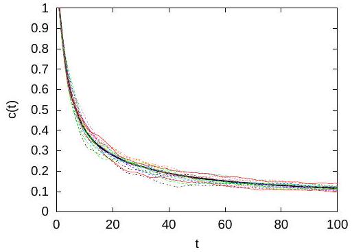
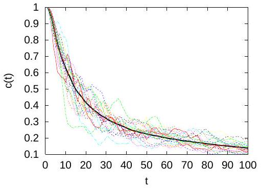
Remark 4. The choice of a which does not include the solvent among the ensemble of species concentration is more appropriate for the case of dilute solutions (see Remark 1). With this choice, equation (30) is still valid for advection-diffusion-reaction processes if the approximation may be adopted. Such an "ergodic" behavior is illustrated in Figure 1, where the concentration at the plume’s center of mass, averaged across the mean flow direction, is close to the mean (thick line) if the initial condition of the transport problem is a narrow plume with large transverse dimensions [3,11]. The opposite situation of non-ergodic behavior, presented in Figure 2, corresponds to a point-like initial condition. Within the ergodic approximation, the concentration PDF can be approximated by the conditional PDF , even if is not constant. Since then , the Fokker-Planck equation solved by may be approximated by equation (2).
5 Numerical solution by global random walk
The particle methods used in classical PDF approaches do not provide a direct solution to the system of Itô equations (3)-(4) associated to the PDF equation (2). Instead, "notional particles" are defined by their position and a "composition" of species concentrations . Then, equation (4) is solved for each particle, all particles are tracked in the physical space according to equation (3), and finally, mean values and PDFs are estimated by particle densities in cells of the physical space [1]. This approach suffers from the increase of computational cost with the number of particles and is affected by numerical diffusion due to the need to interpolate coefficients defined by mean values over cells to particle positions.
As an alternative, we have proposed [7] a global random walk (GRW) approach to solve the Fokker-Planck equation (30) in a mathematically consistent manner, by equivalence between Itô and Fokker-Planck representations of diffusion processes. The GRW solution is related to a suitably weighted concentration PDF by consistency requirements of form (26).
In the next section the GRW-PDF approach will be applied to a two dimensional PDF problem for the joint concentration-position PDF which, under ergodic conditions (see Remark 3), solves a particular form of equation (2),
| (37) |
The system of Itô equations corresponding to (37) takes the form
| (38) | |||
| (39) |
where and are two independent standard Wiener processes.
The solution of the Fokker-Planck equation (37) is approximated by the point-density at lattice sites of a large number of computational particles governed by equations (38) and (39). The computational particles from one lattice site are globally scattered in groups of particles which remain at the position determined by the drift coefficients and of particles undergoing diffusive jumps. The number of particles in each group are binomial random variables with parameters determined by the coefficients of the Itô equations (38) and (39), the time step , and the lattice constants and . The GRW algorithm may
thus be thought as a superposition on a regular lattice of a large number weak Euler schemes for the above system of Itô equations [3,12].
The global scattering of particles from a lattice site ( ) = at time and the update of the particle distribution, 1 ), are described by the relations
| (40) | ||||
| (41) |
where , and are discrete dimensionless parameters corresponding to the drift and diffusion coefficients of the Fokker-Planck equation (37) [7]. The constraints
| (42) |
render the GRW algorithm completely free of numerical diffusion.
The GRW algorithm avoids the numerical diffusion caused by cell averages in classical PDF approaches, because all density estimates are done for lattice nodes, and is practically insensitive to the increase of the number of particles. The reader is referred to [3,12] for implementation details and convergence estimations and to [13, 14] for comparisons with classical numerical schemes. The speed-up with respect to sequential particle-tracking algorithms, of the order of the number of particles (determining the computing time in sequential algorithms) over the number of lattice points occupied by particles (determining the GRW time) [7], is also considerable in real life problems (e.g. billions of particles over millions of grid points [11]). The simulations presented below in Section 7, for about 100000 lattice points and particles took about 0.5 seconds.
6 Parameterization for a problem of transport in groundwater
Monte Carlo simulations of two-dimensional passive transport of a single chemical species in saturated aquifers were used to estimate the PDF of
the concentration averaged over the transverse dimension of the computational domain, , estimated at the -coordinate of the plume center of mass, . The initial plume was chosen as a slab with transverse dimension of 100 correlation scales of the random velocity field. The sample-to-sample fluctuations of the cross-section concentration, shown in Figure 1, are small and the ergodic assumption is justified.
The upscaled drift coefficient in the Fokker-Planck equation (37) is the ensemble mean velocity, equal to the velocity of the center of mass day. The upscaled dispersion coefficient is the longitudinal component of the time dependent ensemble dispersion coefficient. The latter is a self-averaging quantity for transport in random velocity fields with finite correlation range considered here. Hence, is efficiently estimated from a single trajectory of diffusion in a realization of the random velocity field [3, Sect. 7.2].
In case of turbulent reacting flows, the drift and diffusion coefficients and which describe the transport of in the concentration space can be estimated by using turbulence models [1, Section 5.2]. However, similar estimations, done for transport in groundwater failed to reproduce the evolution of the Monte Carlo simulated PDF [7]. Much better results were obtained for parameter estimations based on simulated concentration time series [3,7].
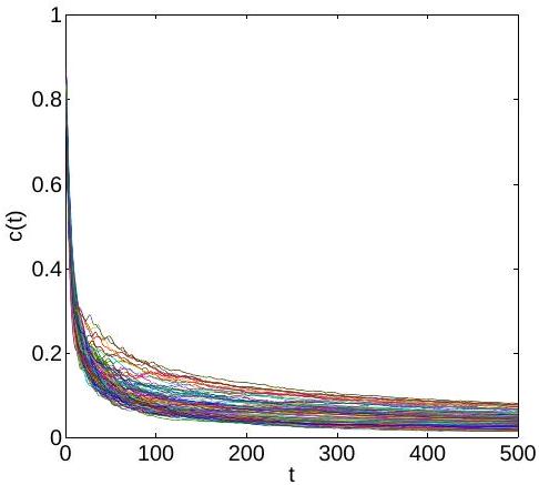
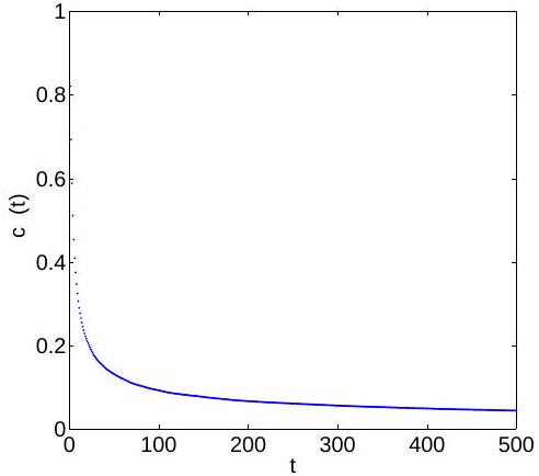
In the following, let us have a closer look at the behavior of such time series. Figures 3 and 4 show 500 time series realizations and the mean time series, respectively, obtained by Monte Carlo simulations of two dimensional

transport with a GRW algorithm [11]. The rate of decay of the mean concentration has been used as a discrete form of the drift displacement in the concentration space . In those papers, it was implicitly assumed that the noise is stationary and Gaussian and the diffusive displacement in the concentration space was simulated by a diffusion coefficient inferred from comparisons with the Monte Carlo simulated PDF.
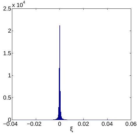
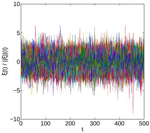
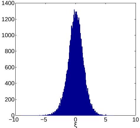
The noisy component of the concentration increments , computed for all 500 time series shows an exponential decay in amplitude (Figure 5). Its histogram (Figure 6) looks more like a function than a Gaussian probability density. In order to refine the analysis, we represent the noise normalized by its maximum amplitude in Figure 7. Now, looks like a white noise and its histogram shown in Figure 8 is close to a Gaussian. Thus, the statistical analysis of the concentration time series supports the assumption that the generic mixing model from (4) can be represented as a sum of drift and diffusion displacements in the concentration space, like in the Itô equation (39). The diffusion coefficient adopted starts from a value day -1 adjusted by comparisons with the Monte Carlo results and decays in exponentially time, similarly to the noise in Figure 5.
7 GRW-PDF simulations
Since the cross-section concentration for the transport process considered here (Section 6) is ergodic with a good approximation, is
well approximated by the conditional PDF (Remark 4). The latter is determined from the concentration-position PDF and position PDF by . The initial distribution of particles in the plane is given by the Monte Carlo PDF at day multiplied by particles. The initial condition and contours for one and particles during the GRW simulation are shown in Figure 9.
Besides the GRW-PDF simulation with parameters presented in Section 6, denoted in the following by GRW1, we also conducted a simulation with drift coefficient in the concentration space given by , for a single realization , instead of the rate of decay of the mean concentration, while keeping the rest of parameters the same. The latter is denoted by GRW2.
Since, according to (20), the mean concentration equals the position PDF , obtained by integrating over the -coordinate the joint PDF , it does not depend on the parameters of the concentration Itô equation (39) and the results for GRW1 and GRW2 are identical (Figure 10).
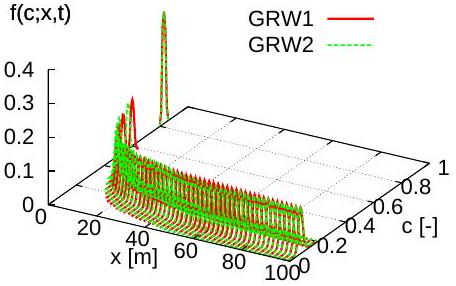
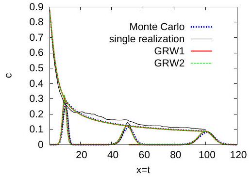
The results for the concentration PDF presented in Figure 11 show more pronounced differences between GRW1 and GRW2 at early times. The cumulative distribution functions presented in Figure 12 allow a better comparison with the Monte Carlo results. One sees that GRW1 provides a quite good approximation of the Monte Carlo result, especially for the transport of the probability distribution in the concentration space. The GRW2 result is also an acceptable approximation of the cumulative distribution and at large times it becomes indistinguishable from the GRW1 approximation.


Remark 5 The good performance of GRW2 simulation can be seen as an indication that mixing models in the form of advection-diffusion in concentration spaces may be obtained by separating the trend and the noise in a single-realization measured concentration time series. Such measurementbased parameterizations could benefit from advanced methods in time series analysis [15] as well as of automatic detrending algorithms [16].
8 Conclusions
The Eulerian random field of concentrations and the Itô process in physical and concentration spaces are distinct stochastic objects and using the latter
to solve the evolution equation for the concentration PDF raises a number of consistency issues. The consistency of such numerical solutions is ensured if the position PDF of the Itô process equals the expectation of a conserved scalar, formed for instance by the sum or by the arithmetic mean of the species concentrations. The concentration-position PDF which solves the associated Fokker-Planck equation gives then the Eulerian concentration PDF weighted by the conserved scalar.
Summarizing Remarks 1-4, we also note that:
-
•
A Fokker-Planck equation equivalent to the system of Itô equations involved in the numerical solution of the PDF problem, consistent with the Eulerian PDF equation, can be derived if the weighting factor is not only a conserved quantity but also obeys a continuity equation, as in case of weighting by the fluid density.
-
•
If the weighting factor is a conserved scalar which does not include the solvent among the species concentrations and it does not verify a continuity equation, then the Fokker-Planck equation can be derived only in an advection-reaction approximation of the full problem or under suitable ergodic assumptions.
-
•
The Fokker-Planck equation takes the form of a diffusion in physical and concentration spaces only if the weighting factor is constant or under ergodic conditions.
The GRW algorithm is a numerical scheme with a robust mathematical foundation for the Fokker-Planck equation associated to the PDF problem and avoids the conceptual inconsistencies and the high computational cost of the classical PDF methods.
The good results obtained by using a single concentration time series to parameterize the concentration evolution equation (39) suggest the possibility to derive parameterizations from measurements. In this paradigm, the position Itô equation (38) can be obtained by standard upscaling methods, while the concentration equation (39) can be inferred by detrending time series of measured concentrations (see Remark 5). The Fokker-Planck equation (37) is then completely determined by the Itô equations (38)-(39) and its solution gives the weighted Eulerian PDF for problem-specific consistency conditions.
Acknowledgements
This work was supported by the Deutsche Forschungsgemeinschaft-Germany under Grants AT 102/7-1, KN 229/15-1, SU 415/2-1 and by the Jülich Supercomputing Centre-Germany in the frame of the Project JICG41.
References
[1] S.B. Pope, PDF methods for turbulent reactive flows, Prog. Energy Combust. Sci. 11(2) (1985) 119-192.
[2] R.O. Fox, Computational Models for Turbulent Reacting Flows, Cambridge University Press, New York, 2003.
[3] N. Suciu. Diffusion in random velocity fields with applications to contaminant transport in groundwater, Adv. Water Resour. 69 (2014) 114-133.
[4] S.B. Pope, Turbulent Flows, Cambridge University Press, Cambridge, 2000.
[5] D.C. Haworth, Progress in probability density function methods for turbulent reacting flows, Prog. Energy Combust. Sci., 36 (2010) 168-259.
[6] A.Y. Klimenko, R.W. Bilger, Conditional moment closure for turbulent combustion, Progr. Energ. Combust. Sci. 25 (1999) 595-687
[7] N. Suciu, F.A. Radu, S. Attinger, L. Schüler, Knabner, A FokkerPlanck approach for probability distributions of species concentrations transported in heterogeneous media, J. Comput. Appl. Math. (2014), in press (doi:10.1016/j.cam.2015.01.030).
[8] D.W. Meyer, P. Jenny, H.A. Tchelepi, A joint velocity-concentration PDF method for tracer flow in heterogeneous porous media, Water Resour. Res., 46 (2010) W12522.
[9] R. W. Bilger, The Structure of Diffusion Flames, Combust. Sci. Tech. 13 (1976) 155-170.
[10] S. Attinger, M. Dentz, H. Kinzelbach, W. Kinzelbach, Temporal behavior of a solute cloud in a chemically heterogeneous porous medium, J. Fluid Mech. 386 (1999) 77-104.
[11] N. Suciu, C. Vamos, J. Vanderborght, H. Hardelauf, H. Vereecken, Numerical investigations on ergodicity of solute transport in heterogeneous aquifers, Water Resour. Res. 42 (2006) W04409.
[12] C. Vamoş, N. Suciu, H. Vereecken, Generalized random walk algorithm for the numerical modeling of complex diffusion processes, J. Comp. Phys., 186 (2003) 527-544.
[13] F. A. Radu, N. Suciu, J. Hoffmann, A. Vogel, O. Kolditz, C-H. Park, S. Attinger, Accuracy of numerical simulations of contaminant transport in heterogeneous aquifers: a comparative study, Adv. Water Resour. 34 (2011) 47-61.
[14] N. Suciu, F.A. Radu, A. Prechtel, F. Brunner, P. Knabner, A coupled finite element-global random walk approach to advection-dominated transport in porous media with random hydraulic conductivity, J. Comput. Appl. Math. 246 (2013) 27-37.
[15] C. Vamoş, M. Crăciun, Separation of components from a scale mixture of Gaussian white noises, Phys. Rev. E 81 (2010) 051125.
[16] C. Vamoş, M. Crăciun, Automatic Trend Estimation, Springer, Dortrecht, (2012).
Nicolae SUCIU and Peter KNABNER,
Mathematics Department,
Friedrich-Alexander University Erlangen-Nuremberg,
Cauerstr. 11, 91058 Erlangen, Germany.
Email: {knabner, suciu}@math.fau.de
Lennart SCHÜLER and Sabine ATTINGER,
Faculty for Chemistry and Earth sciences,
University of Jena,
Burgweg 11, 07749 Jena, Germany, and
Department Computational Hydrosystems,
UFZ Centre for Environmental Research,
Permoserstraße 1504318 Leipzig, Germany.
Email: sabine.attinger@ufz.de
Florin A. RADU,
Department of Mathematics,
University of Bergen,
Allegaten 41, 5020 Bergen, Norway.
Email: Florin.Radu@math.uib.no
Călin VAMOŞ and Nicolae SUCIU,
Tiberiu Popoviciu Institute of Numerical Analysis, Romanian Academy,
Str. Fantanele 57, 400320 Cluj-Napoca, Romania.
Email: {cvamos, nsuciu}@ictp.acad.ro