Global random walk (GRW) algorithms, unconditionally stable and free of numerical diffusion, solve parabolic partial differential equations by moving computational particles on regular lattices according to random walk rules Vamosetal2003 . The GRW approach, intensively used in Monte Carlo simulations of diffusion in random velocity fields Suciu2014 , is based on the relationship between the ensemble of trajectories of the diffusion process governed by the Itô equation and the probability density of the process which verifies a Fokker-Planck equation. The strength of the approach is that instead of sequentially generating random walk trajectories one counts the number of particles at lattice sites, updated according to the binomial distributions which describe the number of jumps to neighboring lattice sites. Since the total number of particles is arbitrarily large, one obtains in this way highly accurate numerical approximations of the probability density, which, in case of transport simulations, is the normalized concentration of the solute that is transported by advection and diffusion.

The second order differential operator of the Fokker-Planck equation coincides with the diffusion operator in the mass balance equation with closure given by the Fick’s law only if the diffusion coefficient is constant. Otherwise, in order to rewrite the diffusion equation as a Fokker-Planck equation, the drift coefficients have to be augmented with the spatial derivatives of the diffusion coefficients (e.g., (Suciu2019, , Sect. 4.2.1)). The same procedure can be used to write the pressure equation for flow in porous media based on Darcy’s law (e.g., Raduetal2011 ) as a Fokker Planck equation. Further, numerical solutions of the flow problem can be obtained by solving the problem formulated for the equivalent Fokker-planck equation by GRW methods.

In case of highly variable coefficients, the particles may jump over several lattice sites, the variability of the coefficients is smoothed, and the GRW solutions are affected by overshooting errors SuciuandVamos2006 . Such errors are avoided by using biased-GRW algorithms, where the particles are only allowed to jump to neighboring sites and the advective displacements are accounted for by biased jump probabilities that are larger in the direction of the drift (Suciu2019, , Sect. 3.3.3). A different remedy, appropriate for GRW solutions of the flow problem, consists of approximating directly the second order operator in diffusion form, with flux terms estimated at the middle of the lattice intervals by using staggered grids (Suciu2019, , Sect. 3.3.4.1).

We consider a two-dimensional domain, $(x,y)\in \mathrm{\Omega }=[0,L_x]\times [0,L_y]$ and the pressure equation for flow in saturated porous media with constant porosity,

where $h(t,x,y)$ is the hydraulic head, $K(x,y)$ is an isotropic hydraulic conductivity, and $f(x,y)$ is a source/sink term. For an arbitrary initial condition (IC) and time independent boundary conditions (BC), the non-steady solution of Eq. (1) approaches a stationary hydraulic head $h(x,y)$. With $f=0$ and BC given by

the gradient of the hydraulic head $h(x,y)$ determines the components of the divergence-free velocity field according to Darcy’s law

The GRW solutions presented in the following are tested against analytical manufactured solutions Roache2002 obtained from data files and codes given in the Git repository https://github.com/PMFlow/FlowBenchmark. The isotropic hydraulic conductivity is a space random function with mean $⟨K⟩=15$ m/day. The random fields $\ln K$ are normally distributed, with Gaussian correlations of fixed correlation length $\lambda =1$ m and increasing variances ${\sigma }^2=0.1,\mathrm{\hspace{0.33em}1},\mathrm{\hspace{0.33em}2}$, with realizations generated as sums of a finite number $N=100$ of cosine random modes (Suciu2019, , Appendix C.3.1.2).

The three different GRW approaches discussed in Section 1 are tested in the following by solving the one-dimensional (1D) version of Eq. (1) written as an advection-diffusion equation,

in the interval $(0,L)$, $L=200\lambda$. The source $f$ and the BCs $h(0)$ and $h(L)$ are determined by the manufactured solution $\tilde{h}(x)=3+\sin (x)$ (see Git repository, /FlowBenchmark/Manufactured_Solutions/Matlab/Gauss 1D/). The precision of the numerical solution $h(x)$ is quantified by the discrete $L^2$ norm $\epsilon ={\Vert h-\tilde{h}\Vert }_{L^2}$.

GRW algorithms approximate the hydraulic head by the distribution $n(i,k)$ at lattice sites $i$ and times $k$ of a system of $𝒩$ random walkers, $h(i\mathrm{\Delta }x,k\mathrm{\Delta }t)\approx n(i,k)/𝒩$. The unbiased GRW moves groups of particles on the lattice according to

where $\lfloor \cdot \rfloor$ is the floor function, $v_j=\lfloor V_j\mathrm{\Delta }t/\mathrm{\Delta }x+0.5\rfloor$, $V_j=\frac{\partial K}{\partial x}(j\mathrm{\Delta }x)$, are discrete advective displacements, and $d$ is the amplitude of the diffusive jumps. The time step $\mathrm{\Delta }t$ and the space step $\mathrm{\Delta }x$ are related by

where $r_j$, $0\le r_j\le 1$, is a variable jump probability. The number of particles undergoing diffusion jumps, $\delta n(j+v_j\mp d,j,k)$, and the number of particles waiting at $j+v_j$ over the $k$ time step, $\delta n(j+v_j,j,k)$, are binomial random variables with mean values given by (Suciu2019, , Sect. 3.2.2)

In the biased GRW algorithm $d=1$ and Eq. (6) is replaced by

The quantities $\delta n$ verify in the mean

where $v_j=V_j\delta t/\delta x$. The biased jump probabilities are given by $(r_j\mp v_j)$ with $r_j$ defined by (8) and, in addition to $r_j\le 1$, one imposes the constraint $\mid v_j\mid \le r_j$ (Suciu2019, , Sect. 3.3.3).

Alternatively, a GRW solution of the 1D version of the pressure equation (1),

can be obtained as steady-state limit of the staggered finite difference scheme

With jump probabilities defined by $r(i\mp 1/2)=K(i\mp 1/2)\mathrm{\Delta }t/\mathrm{\Delta }{x}^2$, $r\le 1/2$, the staggered scheme becomes

The contributions to lattice sites $i$ from neighboring sites summed up in (9) are obtained with the GRW algorithm which moves particles from sites $j$ to neighboring sites $i=j\mp 1$ according to

For consistency with the staggered scheme (9), the quantities $\delta n$ in (11) have to satisfy in the mean (Suciu2019, , Sect. 3.3.4.1),

The three GRW algorithms from above approximate the binomial random variables $\delta n$ by rounding of the unaveraged relations for the mean, e.g., (11), summing up the reminders of multiplication by $r$ and of the floor function $\lfloor 𝒩f\mathrm{\Delta }t\rfloor$, and allocating a particle to the lattice site where the sum reaches the unity. By giving up the particle indivisibility, one obtains deterministic GRW algorithms which represent the solution $n$ by real numbers and use the anaveraged relations for $\delta n$.

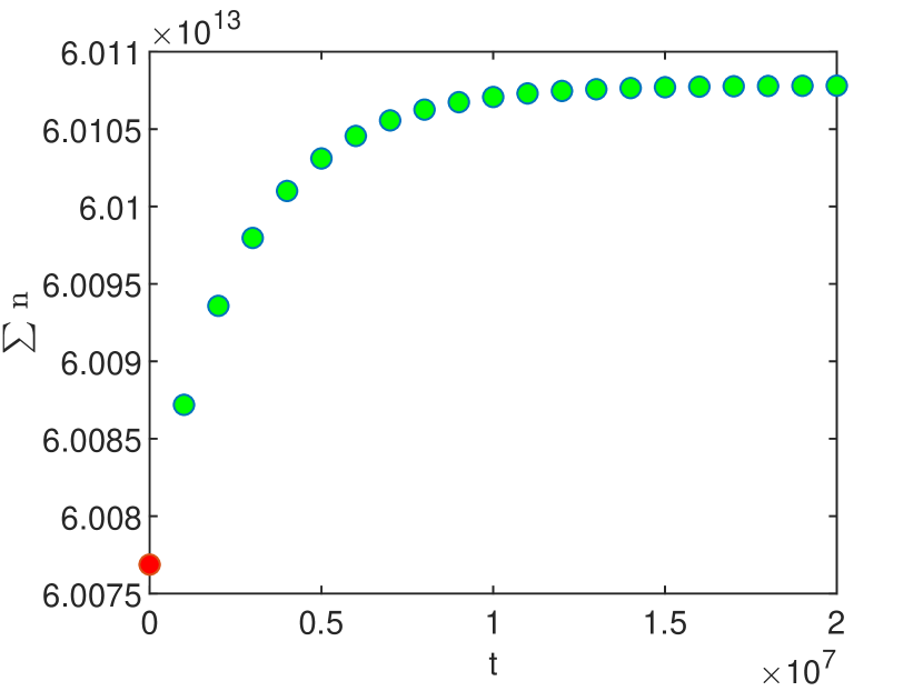
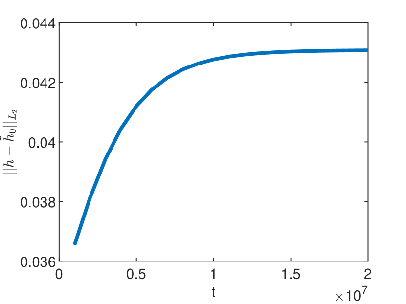
Since the unbiased GRW algorithm is prone to large overshooting errors, due to the high variability of the coefficients $\frac{\partial K}{\partial x}$ and $K$, it is not appropriate to solve the flow problem. For instance, to solve the test problem for ${\sigma }^2=0.1$ with errors $\epsilon \sim {10}^{-1}$, an extremely small step $\mathrm{\Delta }x={10}^{-5}$ is needed and one time iteration takes about 8 minutes. Efficient solutions can be obtained with the biased GRW algorithm (Method 1) and the GRW on staggered grids in both the random (Method 2) and the deterministic implementation (Method 3). The stationary regime of the GRW simulations, indicated by constant total number of particles and $L^2$ error (see Fig 1), is reached after $T=2\cdot {10}^7$ time iterations. The comparison shown in Table 1 indicates that the deterministic implementation of the GRW on staggered grids is the most efficient approach to solve flow problems for heterogeneous porous media.

The 2D GRW algorithm on staggered grids is defined similarly to (9-11) as follows:

The problem (1-3), with $L_x=20\lambda$, $L_y=10\lambda$, $H=1$, $\mathrm{\Delta }x=\mathrm{\Delta }y={10}^{-1}$, and IC given by the manufactured solution, $h_0(x,y)=\tilde{h}(x,y)=1+\sin (2x+y)$, is solved by the deterministic GRW on staggered grids. The $L^2$ errors with respect to the manufactured solution are shown in Table 2.

The convergence of the 2D GRW solutions is investigated for the homogeneous problem ($f=0$, and IC given by the constant slope $h_0(0,y)=1,h_0(L,y)=0$), for increasing ${\sigma }^2$, by successively halving the step size five times from $\mathrm{\Delta }x=\mathrm{\Delta }y={10}^{-1}$ to $\mathrm{\Delta }x=\mathrm{\Delta }y=3.125\cdot {10}^{-3}$. Using the errors with respect to the solution on the finest grid, ${\epsilon }_k={\Vert h^{(k)}-h^{(6)}\Vert }_{L^2}$, the estimated order of convergence (EOC) is computed according to $EOC=\log \left({\epsilon }_k/{\epsilon }_{k+1}\right)/\log (2),k=1,\mathrm{\dots },4$. The results presented in Table 3 indicate the convergence of order 2 for all the three values of ${\sigma }^2$.

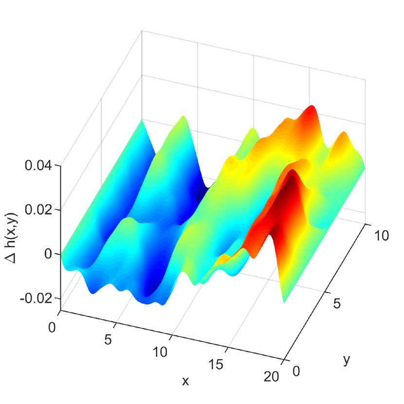
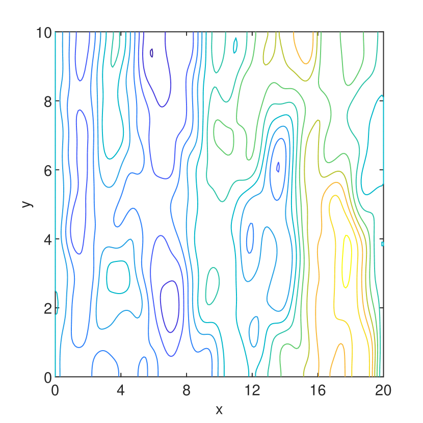
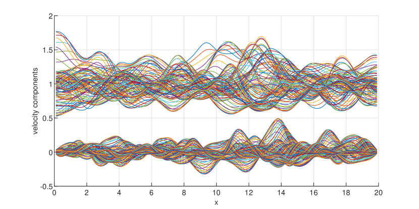
A Monte Carlo ensemble of solutions is obtained by solving the 2D homogeneous problem ($f=0$) for 100 realizations of the random $K$-field with fixed ${\sigma }^2=0.1$. A realization of the hydraulic head is shown in Fig 2. The components of the velocity field computed according to Darcy’s law (4) are shown in Fig. 3.

The Monte Carlo estimates presented in Table 4 are close to the first-order theoretical predictions of the stochastic theories of flow and transport in groundwater Dagan1989 , e.g. variances of the order ${\sigma }_h^2\sim {(\sigma \lambda H/L_x)}^2\sim {10}^{-4}$ for the hydraulic head, ${\sigma }_{V_x}^2=\frac{3}{8}{\sigma }^2=3.75\cdot {10}^{-2}$, and ${\sigma }_{V_y}^2=\frac{1}{8}{\sigma }^2=1.25\cdot {10}^{-2}$, for longitudinal and transverse velocity components, respectively.

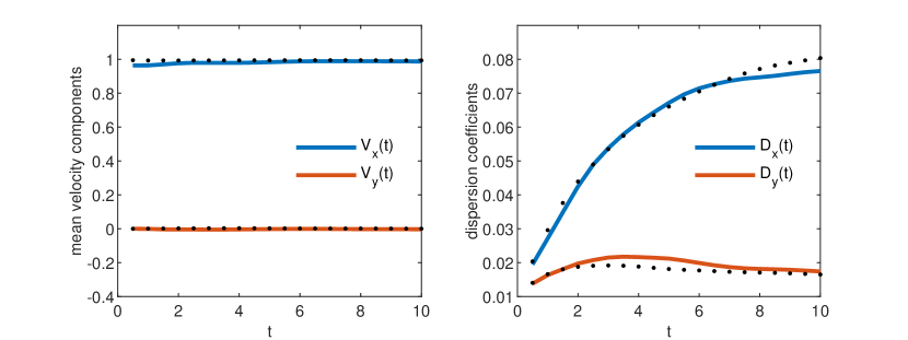
The numerical setup from Section 4 corresponds to a possible scenario of contaminant transport in groundwater systems with low heterogeneity Suciu2014 . With a typical value of the local dispersion coefficient $D_0=0.01$ m²/day, Monte Carlo simulations of advection-diffusion are carried out using the ensemble of 100 velocity fields, on the same lattice as that used in Section 4 to solve the flow problem. The transport problem is solved with the 2D generalization of the unbiased GRW algorithm (6-7) (Suciu2019, , Appendix A.3.2). The Monte Carlo estimates of the velocity of the plume’s center of mass and of the effective dispersion coefficients presented in Fig. 4 are in good agreement with the first-order results obtained from simulations using a linear approximation of the velocity field (Suciu2019, , Appendix C.3.2.2).

References

- (1) Dagan, G.: Flow and Transport in Porous Formations. Springer, Berlin (1989) https://doi.org/10.1007/978-3-642-75015-1
- (2) Radu, F.A., Suciu, N., Hoffmann, J., Vogel, A., Kolditz, O., Park, C-H., Attinger, S.: Accuracy of numerical simulations of contaminant transport in heterogeneous aquifers: a comparative study. Adv. Water Resour. 34, 47–61 (2011) http://dx.doi.org/10.1016/j.advwatres.2010.09.012
- (3) Roache, P.J.: Code verification by the method of manufactured solutions. J. Fluids Eng. 124 (1):4–10 (2002) http://dx.doi.org/10.1115/1.1436090
- (4) Suciu, N.: Diffusion in random velocity fields with applications to contaminant transport in groundwater. Adv. Water Resour. 69 (2014) 114-133. http://dx.doi.org/10.1016/j.advwatres.2014.04.002
- (5) Suciu, N.: Diffusion in Random Fields. Applications to Transport in Groundwater. Birkhäuser, Basel (2019) https://doi.org/10.1007/978-3-030-15081-5
- (6) Suciu, N., Vamoş, C.: Evaluation of overshooting errors in particle methods for diffusion by biased global random walk. Rev. Anal. Num. Th. Approx. (Romanian Academy) 35, 119–126 (2006) https://ictp.acad.ro/jnaat/journal/article/view/2006-vol35-no1-art17
- (7) Vamoş, C., Suciu, N., Vereecken, H.: Generalized random walk algorithm for the numerical modeling of complex diffusion processes. J. Comput. Phys., 186, 527-544 (2003) https://doi.org/10.1016/S0021-9991(03)00073-1.