Abstract
Time series generated by a complex hierarchical system exhibit various types of dynamics at different time scales. A financial time series is an example of such a multiscale structure with time scales ranging from minutes to several years. In this paper we decompose the volatility of financial indices into five intrinsic components and we show that it has a heterogeneous scale structure. The small-scale components have a stochastic nature and they are independent 99% of the time, becoming synchronized during financial crashes and enhancing the heavy tails of the volatility distribution. The deterministic behavior of the large-scale components is related to the nonstationarity of the financial markets evolution. Our decomposition of the financial volatility is a superstatistical model more complex than those usually limited to a superposition of two independent statistics at well-separated time scales.
Authors
Keywords
Computational Methods; superstatistics; econophysics; financial time series analysis; volatility; multiscale structure; nonstationarity of financial markets evolution
Paper coordinates
C. Vamoş, M. Crăciun, Intrinsic superstatistical components of financial time series, The European Physical Journal B 87 (2014): 301, pp. 9,
doi: 10.1140/epjb/e2014-50596-y
References
see the expanding block below.
About this paper
Journal
The European Physical Journal B
Publisher Name
Springer Berlin Heidelberg
Print ISSN
1434-6028
Online ISSN
1434-6036
Paper (preprint) in HTML form
Intrinsic spectral components of complex multiscale time series
Abstract
Time series generated by a complex hierarchical system exhibit various types of dynamics at different time scales. We design an adaptive numerical algorithm to decompose complex multiscale time series into several intrinsic components with minimum spectral superposition. As an application, we decompose the financial volatility into five intrinsic components and we show that it has a heterogeneous scale structure. The small-scale components have a stochastic nature and they are independent 99% of the time, becoming synchronized during financial crashes and enhancing the heavy tails of the volatility distribution. The deterministic behavior of the large-scale components is related to the nonstationarity of the financial markets evolution. Our decomposition of the financial volatility is a superstatistical model more complex than those usually limited to a superposition of two independent statistics at well-separated time scales.
PACS:
05.45.Tp, 89.65.Gh, 05.70.LnI Introduction
In the last two decades the physicists have become more and more interested in complex systems with hierarchical structure extending over many scales costa11 . They are modeled by graphs including modules of different sizes which are grouped in a hierarchical manner baraba03 . A time series generated by such a complex system contains in a compressed form all the intricacies of its complex evolution. Hence one needs special algorithms to identify, separate, and analyze the evolution at different scales of a complex multiscale time series gao07 .
Usually the spectral analysis is realized in a nonadaptive manner, the time series being projected on a predetermined frequency grid, most often equidistant. This is the case even with the most popular multiresolution analysis supplied by the wavelet decomposition percival00 . A better approach would be a data-driven numerical algorithm which should separate several intrinsic spectral components arranged in an increasing hierarchy of frequencies. For a correct characterization of the dynamics over different time scales, an essential issue is the proper separation of time scales between the intrinsic components. Otherwise, we risk to assign to a specific time scale a mixture of unrelated dynamics. The only algorithm known to us which adapts to the characteristics of nonlinear and nonstationary time series is the empirical mode decomposition (EMD) method huang98 . But the EMD components are not constrained with respect to their spectral overlapping.
In this paper we present a numerical algorithm which is not only adaptive, but also decomposes a complex multiscale time series into several intrinsic components with minimum spectral superposition. Our decomposition algorithm is based on the condition that the spectral width of each intrinsic component should be minimum and disjoint from that of the neighboring components.
We test our decomposing algorithm by applying it to a financial time series which is one of the most known example of hierarchical multiscale time series dacoro2001 . In financial markets the time scales range continuously from minutes, where the market makers act, up to several years, intervals characteristic for investment funds. All these investors interact with each other. Asset prices are also influenced by many exterior economic and financial factors with even larger time scales (see for example Chap. 9 in tsay2010 ). Our decomposition algorithm allows us to show that the financial volatility contains a hierarchy of time scales with a heterogeneous scale structure and different dynamical properties. The small-scale intrinsic components have a random nature while the large-scale intrinsic components have a deterministic behavior rendering the financial time series nonstationary.
The statistical mechanics of the complex systems with a hierarchy of temporal or spatial scales is given by a superposition of several statistics, known as superstatistics beck03 ; beck11 . The simplest form of the superstatistical model has only two separate scales with independent random dynamics. For example, the small-scale dynamics may describe a system in local thermodynamical equilibrium with a Boltzmann-Gibbs factor . If the intensive parameter slowly fluctuates at much larger scales, then the statistics of the whole system is given by the mixture of the microscopic statistics
| (1) |
where is the probability distribution function (pdf) of the parameter . The resulting statistics generally have non-Gaussian properties with heavy tails beck03 . The essential supposition in this approach is the independence of the two scales, not their number. If there are several independent time scales, the integral in Eq. (1) is replaced by a multiple integral sobyanin11 .
Many complex systems in various areas of science have been successfully modeled by this simple superstatistical model: turbulence, astrophysics, quantitative finance, climatology, random networks, medicine, etc. beck09 . Remarkable results are obtained when the local equilibrium hypothesis holds as, for example, in turbulence beck07 . But for biological or social systems this hypothesis is unlikely to stand all the time and then the global pdf is no more a simple integral as in Eq. (1) because we have to take into account the interactions between the different time scales. In this paper we show that in most of the time the random small-scale intrinsic components of the financial volatility have an independent evolution, but they become synchronized during financial crashes. Therefore a financial market seems to be a more complex system than a statistical system in local equilibrium in a slowly evolving environment.
II Financial volatility time series
The basic quantity in quantitative finance is the logreturn defined as , where are the prices of a financial asset. The basic properties of daily financial returns, the so-called stylized facts cont01 , are captured by the heteroscedastic model
| (2) |
where is a Gaussian white noise with zero mean and unit variance and is a stochastic process called volatility with strictly positive values and independent of taylor07 . It is a particular case of the superstatistical model. If in Eq. (2) the volatility fluctuates much slowly than the Gaussian noise, then the pdf of the logreturns is a mixture of Gaussians
| (3) |
where is the pdf of the volatility. The superstatistical model has been successfully applied to several financial time series straet09 ; gerig09 ; vamos2010 ; vamos2013 .
In Fig. 1(a) we plot the daily returns computed from the daily closing values of the S&P500 index from 1 January 1950 to 28 July 2012, a time series containing values. The volatility is obtained as the moving average (MA) of the absolute values of the logreturns liu99
| (4) |
where is the semilength of the averaging window and . If (), then the average is taken over the first (the last ) values of . The properties of this MA with normalized padding with zero at boundaries are analyzed in vamos2012 .

Figures 1(b) and (c) show the volatility and the noise estimated by an MA with such that the small scale fluctuations of the volatility are preserved vamos2010 ; vamos2013 . The estimated noise is Gaussian [Fig. 2(a)] but it is uncorrelated only for lags larger than 5 days [Fig. 2(b)] due to the spurious correlations introduced by the MA (see Appendix B in vamos2012 ). Then the estimated volatility is accurate only for time scales larger than 5 days and its intrinsic components may be determined only for these time scales.
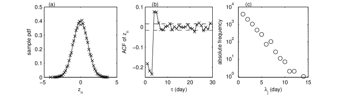
To measure the components spectral width we need a flexible local measure suited for a complex time series. Time scales are usually defined as the periods of the constant-amplitude trigonometric components of the Fourier decomposition. Instead of such a global averaged description, we use the characteristic times defined as the spacings between successive local extrema of the time series, also equal to the lengths of its monotonic segments huang98 . For an arbitrary time series we denote the characteristic times by , . In the simplest cases, the set supplies a full description of the time series spectrum. For instance, a harmonic oscillation has all equal to half the oscillation period.
The situation is more complex in the case of a noisy time series. The characteristic times distribution is dominated by the small-scale fluctuations of the noise and it does not distinguish the large-scale variations possibly existing in the time series. Quantitatively, a time series cannot contain monotonic variations smaller than , but there may exist components with monotonic variations lasting longer than . For instance, the histogram of the characteristic times of the estimated volatility of the S&P500 index is dominated by fluctuations with characteristic times smaller than [Fig. 2(c)], which are much smaller than the characteristic times of the large-scale components of the volatility. Our goal is to decompose the volatility into a hierarchy of spectral components with characteristic times larger than 5 business days, such that the intervals associated to them should be disjoint.
III Decomposition algorithm
We will decompose the volatility into components
| (5) |
where is the mean volatility and are the volatility residuals of order . This is a generalization of the superstatistical model with two independent scales described in the previous section. First, the number of the time scales is not limited to two. If they are independent, then the integral in Eq. (3) is replaced by a multiple integral sobyanin11 . Here we allow that the evolutions at different scales may be correlated and then the global pdf cannot be computed as an integral. Also, the residuals may be non-Gaussian. Finally, we make no assumption on the nature of the components (deterministic or random). In this section we describe the numerical decomposition algorithm and in the next section we exemplify how it works in the case of the S&P500 index.
Similar to the SiZer algorithm chaudhuri99 , we compute the components by successive smoothings, which gradually eliminate the variations with the largest characteristic times from the previous component. Let us assume that the first components have been computed. We denote by the interval containing its characteristic times () equal to the lengths of the monotonic segments. The next component is determined such that the interval should have minimum width and should be as close as possible to the previous interval . In this way the time scales of the components are not predetermined, but they are controlled by data themselves and the resulting algorithm has an adaptive nature.
For smoothing we use the repeated central MA (RCMA) with normalized padding with zero at boundaries (Chap. 4 in vamos2012 ) obtained by repeating the smoothing (4) several times. Its parameters are the semilength of the averaging window and the number of repetitions of the MA. Roughly the same smoothing is realized by averaging many times with a small or several times with a large vamos2012 . Therefore we maintain between 15 and 20 repetitions and we vary mainly the semilength from one component to the next.
We denote by the time series obtained after one application of the RCMA to the residuals of order , and by that obtained after a second application to . It is possible that a single smoothing with the RCMA cannot extract all the variations with the characteristic times in . If the most part of the monotonic segments with characteristic times in has not been extracted, i.e., if , where is the quadratic norm, then we apply once again the RCMA to the new partial residuals . We stop the averagings after iterations when the quadratic norm of is one order of magnitude smaller than that of the product .
After several applications of the RCMA, there remain some monotonic segments with reduced lengths and amplitudes which are not related to the characteristic times within of the component. A large-scale monotonic variation may be separated into two shorter segments with the same monotony by a small inflexion with opposite monotony. We replace these three segments by a single monotonic segment with the length equal to the sum of the three lengths using the ACD algorithm designed to determine the monotonic component of an arbitrary time series vamos2007 ; vamos2012 . In this way the three initial characteristic times are replaced by a single one equal to their sum so that the interval is shifted towards the larger values of the characteristic times. We eliminate the small monotonic segments in ascending order of their lengths until does not overlap . We choose the parameters of the RCMA and the number of the ACD iterations such that the resulting interval has a minimum width.
IV Volatility intrinsic components
IV.1 The first two volatility intrinsic components
Before applying the adaptive iterative procedure presented in the previous section to identify the intrinsic components of the estimated volatility, we need to know the initial largest-scale component. We determine it such that the adaptive nature of the whole algorithm should not be endangered. We satisfy this goal by imposing the condition that the global shape of the largest-scale component should be preserved by applying additional smoothings.
In order to obtain a strong smoothing of the volatility time series we apply the MA (4) with a large value of the averaging window . We repeat the averaging 20 times and for each number of averagings we compute the number of monotonic segments of the averaged time series [Fig. 3(a)]. After the first averaging the number of monotonic segments is reduced from 7842 contained by the initial time series down to 16. The next variations of occur only at some values of and are much smaller than the first one.
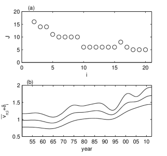
In Fig. 3(b) we plot three of the averaged time series corresponding to some of the main jumps of . After averagings the averaged volatility has monotonic segments and the shortest of them with 877 business days begins in 1975 and ends at 1978. The next three averagings preserve the number of monotonic segments but the length of the shortest one is reduced to 196 business days and its amplitude decreases. This monotonic segment and that beginning in 2001 and ending at 2004 are simultaneously eliminated by the 10th averaging, so that the number of the monotonic segments becomes . Now the shortest monotonic segment has 1232 business days and is situated at the beginning of the averaged time series. It is eliminated by the 18th averaging after which there remain only 4 monotonic segments. A detailed analysis of the repeated averagings effect on the local extrema can be found in Chap. 6 of vamos2012 .
Additional averagings do not reduce the number of the monotonic segments and therefore we consider that the estimated volatility averaged 18 times describes the largest-scale monotonic variations of the volatility. It contains four time intervals: two with almost constant averaged volatility, only slightly decreasing (from 1950 to 1965 and from 1980 to 1995) and two with increasing averaged volatility (1970s and after 1995 to 2012). The global shapes of the averaged volatilities for do not significantly differ from each other, except for several fluctuations with small amplitudes.
The averaged volatility has an obvious global increasing component over which the four monotonic segments described above are superposed [Fig. 3(b)]. This superposition alters the characteristic times, increasing those for the increasing segments and decreasing the others. Therefore, by means of the ACD algorithm vamos2012 , we separate the global monotonic component of the averaged volatility and we identify it with the first component of the volatility [continuous line in Fig. 4(b)].
We may not identify the second volatility intrinsic component with because we are not sure that we have successfully extracted the most part of the largest-scale variations of the volatility. Therefore we apply the RCMA with and several time to the residuals (Sect. III). In Fig. 5(a) we plot the first five partial averages and we observe that their amplitudes progressively diminish with , while preserving approximately the same shape. We neglect the fifth partial average and we retain only the first four partial averages because .
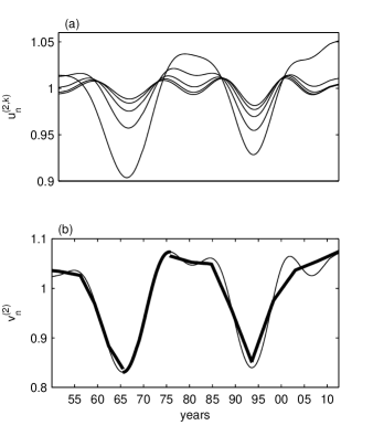
Finally we eliminate by means of the ACD algorithm the insignificant monotonic segments from the product . The shortest monotonic segment has 973 business days and lasts from 1980 to 1984 [Fig. 5(b)]. After its elimination, the resulting decreasing segment has 4409 business days. The second monotonic segment which we eliminate has 1195 business days and lasts from 2001 to 2006 and the resulting increasing segment has 4761 business days. Finally, the third eliminated monotonic segment lays at the left boundary of the time series and then the ACD algorithm is applied only to two neighboring monotonic segments. By applying the ACD algorithm, the number of the monotonic segments diminishes from 9 to 4 and their lengths range between 10 and 19 years. The final result is the second intrinsic component [dashed line in Fig. 4(b)].
IV.2 Heterogeneous spectral structure of volatility
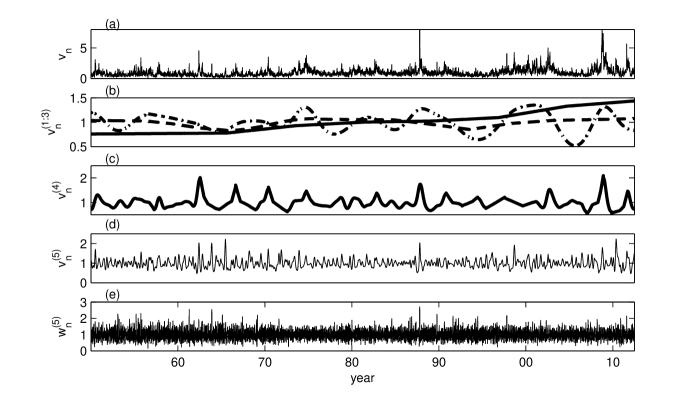
The next three intrinsic components are obtained with the iterative method described in Sect. III taking as reference the interval [Figs. 4(b-d)]. We applied the RCMA algorithm three times with , , and and . The ACD algorithm was applied one time, 20 times, and 37 times, respectively. We analyze the spectral properties of the intrinsic components plotting the overall variations of the monotonic segments as a function of their lengths, i.e., their characteristic times (Fig. 6). The first component is monotonic and has a single characteristic time equal to the time series length (not plotted in Fig. 6).

The third intrinsic component [point-dashed line in Fig. 4(b)] has the characteristic times ranging from 3 to 8.5 years (asterisks in Fig. 6). The characteristic times of the forth and fifth intrinsic components [Figs. 4(c) and (d)] range between half a year to 2.6 years, and one to six months, respectively (triangles and crosses in Fig. 6). The residuals [Fig. 4(e)] have characteristic times between one and 12 days (point markers in Fig. 6). We have to take into account that the characteristic times shorter than 5 days of are not reliable, because they are mixed with those of the estimated noise in Eq. (2).
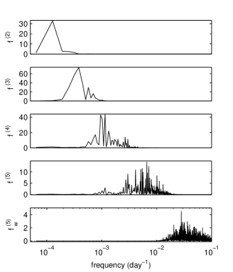
The volatility intrinsic components have been determined such that their characteristic times are rigourously disjoint (Fig. 6). As discussed in Sect. III, there is a possibility that the neighboring intrinsic components may have monotonic variations with overlapping characteristic times. Indeed, there exists a superposition of the Fourier time scales but it is minimal, the regions of the maximum power spectra of the intrinsic components being clearly separated (Fig. 7).
In the following, we use this volatility decomposition to analyze the dynamics at different time scales. We can associate a pdf only to the last two intrinsic components and . We can also associate a pdf to the residuals of order five . Their pdfs are very similar (Fig. 8) and they are likely realizations of stationary stochastic processes. Because of their resemblance we group them as the random part of the volatility .

The first two volatility components contain the largest-scales variations and we group them as the deterministic part of the volatility . Even if they were generated by a stochastic process, because of their limited number of values they cannot be distinguished from a deterministic signal. The different nature of these two components from the others is also sustained by their smaller amplitudes of the monotonic segments (Fig. 6).
The shape of the third intrinsic component and its characteristic times can be related to the well-known business cycles schump39 . We interpret it as a transition component between the deterministic and random parts. In this way the estimated volatility is split up into a deterministic part and a random part, the third intrinsic component making the transition between them .
The existence of the deterministic large-scale components means that the volatility is a nonstationary time series brockdav96 . This result supports the alternative approach in quantitative finance, revived in the last decade, which considers that the volatility is not a stochastic process, but a slowly varying deterministic function bellegem11 . Even more similar to our result is the spline-GARCH model in which the volatility is a superposition of a deterministic function and a stationary stochastic process engle08 .
The existence of the deterministic components also means that there is not a unique pdf of the volatility. Because the large-scale components have a deterministic behavior, the global pdf is a discrete summation, not an integral as in Eq. (3) vamos2010 ; vamos2013 . As a consequence, cannot be computed as a universal expression and it depends on the particular form of the deterministic part. This fact could be a possible explanation for the difficulty to determine a general pdf for the financial time series voit2005 .
V Synchronization of intrinsic volatility components
Now we check if the random intrinsic components of the volatility are independent, as the superstatistical model (3) assumes. We can destroy the possible correlations between the three components of by shuffling their values and then multiplying them. The majority of the values of the initial and the shuffled pdfs coincide, proving that most of the time the three random intrinsic components fluctuate independently [Fig. 9(a)]. Their tails differ from each other only for , for 120 values representing 0.76% of all the volatility values. Hence more than 99% of the time the random intrinsic components fluctuate independently and the central part of the resulting pdf can be computed as a multiple integral generalizing Eq. (3). We obtained the same result for two other financial indices, DJI and NIKKEI.
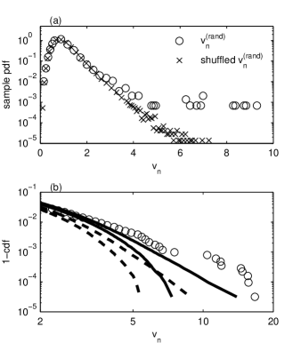
It is well-known that volatility has heavy tails liu99 . The question is if the tail of the volatility random part remains heavy. A pdf with heavy tails has an asymptotic behavior following a power law and its moments of order higher than the absolute value of the exponent are infinite resnick2007 . Because the existing statistical methods to recognize and to measure power law tails have significant errors resnick2007 , we compare the volatility tails with the tails of the Laplace distribution , where is a positive real parameter. We use this distribution as a reference because, unlike the power law distributions, all its moments are finite although it has heavier tails than the Gaussian distribution.
We need several thousands of observations to establish if a sample pdf has heavy or exponential tails heyde04 , condition satisfied by our volatility time series. We have numerically generated 1000 uncorrelated time series with Laplace distribution of unit variance () having the same length as the volatility time series. Then we have computed the cumulative distribution function (cdf) for each artificial time series and we have established the limits containing 95% of the complementary cdf (1 - cdf) [dashed lines in Fig. 9(b)]. We have also generated 1000 shuffled versions of , we have standardized them by extracting their mean and then dividing the result by their standard deviation, and we have established the 95% interval of variation of their complementary cdfs [continuous lines in Fig. 9(b)].
The right tail of the volatility random part is significantly heavier than those of the Laplace distribution [Fig. 9(b)]. This tail is reduced by shuffling, but the tails of the standardized shuffled time series remain almost in all cases heavier than the exponential tails. Hence, even if the random intrinsic components of the volatility were independent, their product would have heavy tails. The correlation between them only enhances their heaviness. In conclusion, the extreme volatility is the result of both the superstatistical mechanism (mixture of different statistics) and the correlation between the random volatility components.
The random intrinsic components of the volatility become correlated during financial crashes when the financial markets structure is reorganized and all the categories of investors act in the same way, i.e., they become synchronized onnela2003b ; mcdonald2008 ; peron2011 . Synchronization of dynamically interacting units in a complex network was observed in a large variety of domains arenas2008 . Hence we have shown that the synchronization of the network structure is accompanied by the temporal synchronization of the dynamics at different time scales.
VI Conclusions
There are many possible applications of our adaptive decomposition algorithm due to its ability to separate nonlinear and nonstationary time series into disjoint intrinsic spectral components. They can be analyzed by usual statistical tests and the possible spectral heterogeneities may be discovered. For instance, the existence of the slowly varying trend in a noisy time series could be separated from a random noise with characteristic times much smaller than those of the trend. Also, one could analyze the intrinsic components of the concentration in an anomalous diffusion process generated by the superposition of a microscopic Brownian motion over a transport through a random porous medium suciu .
Here we have shown that the well-separated spectral intrinsic components of the financial volatility allow the search for correlations between the dynamics at different scales. Generalizing this result we conjecture that the temporal multiscale synchronization of the communities of a complex network may be a general mechanism to generate heavy tails different from those proposed till now as the combination of exponentials, the Yule process, critical phenomena, self-organized criticality newman2005 , the superstatistical model beck03 or the mixture of Gaussians gherghiu04 . The fact that the volatility heavy tails result from the simultaneous action of two distinct such mechanisms indicates that any of these mechanisms could collaborate to generate heavy tails when the system has a hierarchical complex structure.
In accordance with Eq. (2), the complex structure of the volatility is conveyed to logreturns. The heterogeneity of the intrinsic components and the synchronization of small-scale components might provide an explanation for the difficulty to model the logreturn distribution voit2005 . In particular, even if the financial returns have a universal tail index around 3 gopi99 , there exist significant variations between individual companies plerou99 . These variations are small for intraday returns, but they increase for daily returns. The variations are even larger for exchange rates between different currencies dacoro2001 . Such variations can be analyzed in relation with the complex evolution of the intrinsic components obtained with the adaptive decomposition algorithm presented here.
References
- (1) L.F. Costa, O.N. Oliveira, G. Travieso, F.A. Rodrigues, P.R.V. Boas, L. Antiqueira, M.P. Viana, and L.E.C. da Rocha, Adv. Phys. 60, 329 (2011).
- (2) A.L. Baraási, E. Ravasz, and Z. Oltvai, in Statistical Mechanics of Complex Networks, edited by R. Pastoras-Satorras, M. Rubi, and A. Diaz-Guilera (Springer, Berlin, 2003).
- (3) J. Gao, Y. Cao, W. Tung, and J. Hu, Multiscale Analysis of Complex Time Series (Wiley, Hoboken, 2007).
- (4) D.B. Percival and A.T. Walden, Wavelet Methods for Time Series Analysis (Cambridge, Cambridge, 2000).
- (5) N.E. Huang, Z. Shen, S.R. Long, M.C. Wu, H.H. Shih, Q. Zheng, N.C. Yen, C.C. Tung, and H.H. Liu, Proc. R. Soc. Lond. A 454, 903 (1998).
- (6) M.M. Dacorogna, R. Gençay, U.A. Müller, R.B. Olsen, and O.V. Pictet, An Introduction to High-Frequency Finance (Academic Press, San Diego, 2001).
- (7) R.S. Tsay, Analysis of Financial Time Series (Wiley, Hoboken, 2010).
- (8) C. Beck and E.G.D. Cohen, Physica A 322, 267 (2003).
- (9) C. Beck, Phil. Trans. R. Soc. A 369, 453 (2011).
- (10) D.N. Sob’yanin, Phys, Rev. E 84, 051128 (2011).
- (11) C. Beck, Braz. J. Phys. 39, 357 (2009).
- (12) C. Beck, Phys. Rev. Lett. 98, 064502 (2007).
- (13) R. Cont, Quant. Financ. 1, 223 (2001).
- (14) S.J. Taylor, Asset Price Dynamics, Volatility, and Prediction (Princeton University Press, Princeton, 2007).
- (15) E. Van der Straeten and C. Beck, Phys. Rev. E 80, 036108 (2009).
- (16) A. Gerig, J. Vicente, and M.A. Fuentes, Phys. Rev. E 80, 065102 (2009).
- (17) C. Vamoş and M. Crăciun, Phys. Rev. E 81, 051125 (2010).
- (18) C. Vamoş and M. Crăciun, Eur. Phys. J. B 86, 166 (2013).
- (19) Y. Liu, P. Gopikrishnan, P. Cizeau, M. Meyer, C.-K. Peng, and H.E. Stanley, Phys. Rev. E 60, 1390 (1999).
- (20) C. Vamoş and M. Crăciun, Automatic Trend Estimation (Springer, Dordrecht, 2012).
- (21) P. Chaudhuri and J.S. Marron, J. Am. Stat. Assoc. 94, 807 (1999).
- (22) C. Vamoş, Phys. Rev. E 75, 036705 (2007).
- (23) J.A. Schumpeter, Business Cycles. A Theoretical, Historical and Statistical Analysis of the Capitalist Process (McGraw-Hill, New York, 1939).
- (24) P.J. Brockwell, R.A. Davies, Time Series: Theory and Methods (Springer Verlag, New York, 1996).
- (25) S. Van Bellegem, in Wiley Handbook in Financial Engineering and Econometrics: Volatility Models and Their Applications, edited by L. Bauwens, C. Hafner, S. Laurent (Wiley, New York, 2011).
- (26) R.F. Engle, J.G. Rangel, Rev. Financ. Stud. 21, 1187 (2008).
- (27) J. Voit, The Statistical Mechanics of Financial Markets (Springer, Berlin, 2005).
- (28) S.I. Resnick, Heavy tails Phenomena. Probabilistic and Statistical Modeling (Springer, New York, 2007).
- (29) C.C. Heyde and S.G. Kou, Oper. Res. Lett. 32, 399 (2004).
- (30) J.P. Onnela, A. Chakraborti, K. Kaski, J. Kertész, and A. Kanto, Phys. Rev. E 68, 056110 (2003).
- (31) M. McDonald, O. Suleman, S. Williams, S. Howison, and N. F. Johnson, Phys. Rev. E 77, 046110 (2008).
- (32) T.K.D. Peron and F.A. Rodrigues, Europhys. Lett. 96, 48004 (2011).
- (33) A. Arenas, A. Díaz-Guilera, J. Kurths, Y. Moreno, and C. Zhou, Phys. Rep. 469, 93 (2008).
- (34) N. Suciu, Phys. Rev. E 81, 056301 (2010).
- (35) M.E.J. Newman, Contemp. Phys. 46, 323 (2005).
- (36) S. Gheorghiu and M.-O. Coppens, PNAS 101, 15852 (2004).
- (37) P. Gopikrishnan, V. Plerou, L.A.N. Amaral, M. Meyer, and H.E. Stanley, Phys. Rev. E 60, 5305 (1999).
- (38) V. Plerou, P. Gopikrishnan, L.A.N. Amaral, M. Meyer, and H.E. Stanley, Phys. Rev. E 60, 6519 (1999).
2. A.L. Barabási, E. Ravasz, Z. Oltvai, in Statistical Mechanics of Complex Networks, edited by R. Pastoras-Satorras, M. Rubi, A. Diaz-Guilera (Springer, Berlin, 2003)Google Scholar3.
3. M.M. Dacorogna, R. Gençay, U.A. Müller, R.B. Olsen, O.V. Pictet, An Introduction to High-Frequency Finance (Academic Press, San Diego, 2001)Google Scholar
4. R.S. Tsay, Analysis of Financial Time Series (Wiley, Hoboken, 2010)Google Scholar
5. C. Beck, E.G.D. Cohen, Physica A 322, 267 (2003)ADSCrossRefzbMATHMathSciNetGoogle Scholar
6. C. Beck, Philos. Trans. R. Soc. A 369, 453 (2011)ADSCrossRefzbMATHGoogle Scholar
7. D.N. Sob’yanin, Phys. Rev. E 84, 051128 (2011)ADSCrossRefGoogle Scholar
8. C. Beck, Braz. J. Phys. 39, 357 (2009)ADSCrossRefGoogle Scholar
9. C. Beck, Phys. Rev. Lett. 98, 064502 (2007)ADSCrossRefGoogle Scholar
10. J. Gao, Y. Cao, W. Tung, J. Hu, Multiscale Analysis of Complex Time Series (Wiley, Hoboken, 2007)Google Scholar
11. D.B. Percival, A.T. Walden, Wavelet Methods for Time Series Analysis (Cambridge University Press, Cambridge, 2000)Google Scholar
12. N.E. Huang, Z. Shen, S.R. Long, M.C. Wu, H.H. Shih, Q. Zheng, N.C. Yen, C.C. Tung, H.H. Liu, Proc. R. Soc. London A 454, 903 (1998)ADSCrossRefzbMATHMathSciNetGoogle Scholar13.
13. R. Cont, Quant. Financ. 1, 223 (2001)CrossRefGoogle Scholar
14. S.J. Taylor, Asset Price Dynamics, Volatility, and Prediction (Princeton University Press, Princeton, 2007)Google Scholar
15. E. Van der Straeten, C. Beck, Phys. Rev. E 80, 036108 (2009)ADSCrossRefGoogle Scholar
17. C. Vamoş, M. Crăciun, Phys. Rev. E 81, 051125 (2010)ADSCrossRefGoogle Scholar
18. C. Vamoş, M. Crăciun, Eur. Phys. J. B 86, 166 (2013)ADSCrossRefGoogle Scholar
19. Y. Liu, P. Gopikrishnan, P. Cizeau, M. Meyer, C.-K. Peng, H.E. Stanley, Phys. Rev. E 60, 1390 (1999)ADSCrossRefGoogle Scholar
20. C. Vamoş, M. Crăciun, Automatic Trend Estimation (Springer, Dordrecht, 2012)Google Scholar
21. P. Chaudhuri, J.S. Marron, J. Am. Stat. Assoc. 94, 807 (1999)CrossRefzbMATHMathSciNetGoogle Scholar
22. C. Vamoş, Phys. Rev. E 75, 036705 (2007)ADSCrossRefGoogle Scholar
23. J.A. Schumpeter, Business Cycles. A Theoretical, Historical and Statistical Analysis of the Capitalist Process (McGraw-Hill, New York, 1939)Google Scholar
24. P.J. Brockwell, R.A. Davies, Time Series: Theory and Methods (Springer-Verlag, New York, 1996)Google Scholar
25. S. Van Bellegem, in Wiley Handbook in Financial Engineering and Econometrics: Volatility Models and Their Applications, edited by L. Bauwens, C. Hafner, S. Laurent (Wiley, New York, 2011)Google Scholar
26. R.F. Engle, J.G. Rangel, Rev. Financ. Stud. 21, 1187 (2008)CrossRefGoogle Scholar
27. J. Voit, The Statistical Mechanics of Financial Markets (Springer, Berlin, 2005)Google Scholar
28. S.I. Resnick, Heavy tails Phenomena. Probabilistic and Statistical Modeling (Springer, New York, 2007)Google Scholar
29. C.C. Heyde, S.G. Kou, Oper. Res. Lett. 32, 399 (2004)CrossRefzbMATHMathSciNetGoogle Scholar
30. J.P. Onnela, A. Chakraborti, K. Kaski, J. Kertész, A. Kanto, Phys. Rev. E 68, 056110 (2003)ADSCrossRefGoogle Scholar
31. M. McDonald, O. Suleman, S. Williams, S. Howison, N.F. Johnson, Phys. Rev. E 77, 046110 (2008)ADSCrossRefGoogle Scholar
32. T.K.D. Peron, F.A. Rodrigues, Europhys. Lett. 96, 48004 (2011)ADSCrossRefGoogle Scholar
33. A. Arenas, A. Díaz-Guilera, J. Kurths, Y. Moreno, C. Zhou, Phys. Rep. 469, 93 (2008)ADSCrossRefMathSciNetGoogle Scholar
34. M.E.J. Newman, Contemp. Phys. 46, 323 (2005)ADSCrossRefGoogle Scholar
35. S. Gheorghiu, M.-O. Coppens, Proc. Natl. Acad. Sci. 101, 15852 (2004)ADSCrossRefGoogle Scholar
36. P. Gopikrishnan, V. Plerou, L.A.N. Amaral, M. Meyer, H.E. Stanley, Phys. Rev. E 60, 5305 (1999)ADSCrossRefGoogle Scholar
37. V. Plerou, P. Gopikrishnan, L.A.N. Amaral, M. Meyer, H.E. Stanley, Phys. Rev. E 60, 6519 (1999)ADSCrossRefGoogle Scholar