Abstract
This paper deals with the light travel time effect in binary systems with variable components. The methods for estimation of the orbital elements relying on the parameters obtained through Fourier decomposition of the respective timing / O − C data, are reviewed. Some new formulae are derived and some qualitative remarks on the adopted methodology are discussed. Finally, some issues related to the presence of time gaps in the analysed data and to the case of noisy data are addressed.
Authors
Alexandru Pop
Astronomical Institute, Astronomical Observatory Cluj-Napoca, Romanian Academy
Maria Crăciun
Tiberiu Popoviciu Institute of Numerical Analysis, Romanian Academy
Mihai Bărbosu
Rochester Institute of Technology, School of Mathematical Sciences, New York, USA
Keywords
Variable stars; Binary systems; Data analysis.
Paper coordinates
A. Pop, M. Crăciun, M. Bărbosu, On the determination of the orbital elements in the light travel time effect, Romanian Astron. J., 32 (2022) no. 1, pp. 59-71.
About this paper
Journal
Romanian Astronomical Journal
Publisher Name
Editura Academiei Romane
DOI
Print ISSN
1220-5168
Online ISSN
2285-3758
google scholar link
Paper (preprint) in HTML form
On the Determination of the Orbital Elements in the Light Travel Time Effect
Abstract
This paper deals with the light travel time effect in binary systems with variable components. The methods for estimation of the orbital elements relying on the parameters obtained through Fourier decomposition of the respective timing / data, are reviewed. Some new formulae are derived and some qualitative remarks on the adopted methodology are discussed. Finally, some issues related to the presence of time gaps in the analysed data and to the case of noisy data are addressed.
keywords:
Variable stars – Binary systems – Data analysis1 Introduction
Unseen companions of variable stars (either pulsating stars or eclipsing close binary systems, or planets around pulsars) can be detected through the well-known Light Travel Time Effect (LTTE). It consists of the modulation of the variable star period induced by the orbital motion around the barycentre of the system (variable star + unseen companion(s)). As a consequence, the occurrence of the corresponding extremum light times is also modulated. The study of the LTTE has been tackled by different authors, like Woltjer (1922), De Sitter (1933), Irwin (1952, 1959), Kopal (1959, 1978) and Borkovits & Hegedüs (1996), Konacki & Maciejewski (1996, 1999), Pop (1998, 1999, 2000). The common goal of their approaches was to estimate the values of the orbital elements for the corresponding system.
Being given a timing data set and choosing the mathematical model which rules the LTTE, the values of the orbital elements are frequently estimated through the Levenberg-Marquardt least-squares minimization method. However, its application requires first/initial guesses of the values of the orbital elements. When the complexity of the investigated period variability phenomenon is relatively high, the identification of the set of initial values which leads towards the optimal fit, can be a real challenge. The solution to this problem, which was adopted by several authors, was to explore a large number of initial guesses (e.g., Hinse et al. 2012a, 2014b; Lee et al. 2014; Borkovits et al. 2015; Esmer et al. 2021).
The aim of the present paper is to review the problem of the estimation of first guesses of orbital elements relying on the parameters of an ephemeris containing a truncated Fourier series (e.g., Pop 1996) and taking into account the Fourier decomposition of the LTTE (see Kopal 1959, 1978; Borkovits & Hegedüs 1996; Konacki & Maciejewski 1996; Pop 1998, 1999, 2000). Some new formulae are derived and different practical aspects are also considered in order to account for the presence of time gaps in the analysed data as well as for the presence of the additive observational noise.
2 The LTTE Model
The occurrence of the extremum (minimum or maximum) light times of a variable star which has an unseen companion (stellar or planetary) is described by the well-known ephemeris (e.g., Kopal 1978)
| (1) |
where is the initial epoch, is the period of the observed variable star, and is the variability cycle number. The last term represents the time delay required to the light to travel across the projection of the radius vector of the variable star orbit onto the line of sight. In the formulae given below, we used the following notations: is the projected semi-major axis of the absolute orbit of the barycentre of the variable component around the barycentre of the hypothetical binary or triple system, is the inclination of the normal to the orbital plane with respect to the line of sight, is the speed of light, is the orbital eccentricity, is the periastron longitude, is the time of periastron passage, and is the orbital period.
When assuming more unseen companions, the LTTE model can also be applied, but only by neglecting the gravitational perturbations between companions (e.g., Hinse et al. 2012b, 2014a).
Taking into account the well-known expansions of the elliptic motion (e.g., Brouwer & Clemence 1961; Townsend & Tamburro 1968; Kopal 1978), we have
| (2) |
| (3) |
with
| (4) |
Thus, Eq. (1) becomes
| (5) |
where
| (6) |
| (7) |
| (8) |
| (9) |
and being the mean anomaly and the dimensionless frequency which features the periodic behaviour of the curve respectively, while is the orbital angular frequency or the mean motion. This way, the LTTE ephemeris (Eq. (1)) becomes
| (10) |
Kopal (1978) rewrote it in the form
| (11) |
with the following notations
| (12) |
| (13) |
From Eqs. (2) and (2) it immediately results
| (14) |
Pop (1998, 1999, 2000) used slightly different notations in Eq. (2):
| (15) |
| (16) |
with
| (17) |
to write the LTTE ephemeris in the form
| (18) |
where
| (19) |
| (20) |
From Eq. (18) one immediately can see that the times of extremum light displayed by a variable star having an unseen companion are modulated by an arbitrary periodic signal, its parameters being functions of the orbital elements of the system, which is a previously known result. Consequently, the amplitude spectrum of the residuals computed from these extremum light times is a line spectrum, consisting of an infinite number of lines situated at the frequencies and having the monotonically decreasing amplitudes [see also Konacki & Maciejewski (1996, 1999)].This characteristic feature is useful, e.g., in the case of Algol type systems, in the situation where we need to make a differential diagnosis with respect to the quasiperiodic modulation induced by the magnetic cyclic activity occurring in the cool, late-spectral type secondary component (e.g., Pop et al. 2017).
The constant term which appears in Eq. (18) is actually included in the observed times of minimum light. In fact, within the frame of our approach, the estimation of initial guesses of the orbital elements relies on the equivalence between the LTTE term in Eq. (1) and the truncated Fourier series appearing in Eqs. (2) and (18) [see also Hinse et al. (2012a)].
3 First guesses of the orbital elements
In this section we present some methods for estimating the values of the orbital elements of the (hypothetical) absolute orbit of the variable star around the system’s barycentre; these elements are: or , , , , and . The value of the orbital period can be immediately calculated from the formula , in which, the values of and resulted from the fitting of the model (2) or (18) to the observational data.
Kopal’s (1978) approach kept the first two periodic terms from the truncated Fourier series appearing in the LTTE ephemeris (Eq. (2)) and after that, formulae for the orbital elements were derived. He also made some approximations in the formulae of the and coefficients:
| (22) |
Therefore, the orbital elements became:
| (23) |
| (24) |
| (25) |
| (26) |
Tests performed by Borkovits & Hegedüs (1996) indicated that reliable results could be obtained with these formulae for .
Borkovits & Hegedüs (1996) also derived corresponding formulae for the case in which the first three periodic terms in Eq. (2) were considered and they also took into account second order approximations in order to estimate the orbital elements. Thus, these approximations for the coefficients and are [see also, e.g., Brouwer & Clemence (1961)]:
| (27) |
| (28) |
| (29) |
The corresponding formulae given by Borkovits & Hegedüs (1996) for the orbital elements become (with our notations)
| (30) |
| (31) |
| (32) |
| (33) |
The approach of Pop (1998, 1999, 2000) relied on the LTTE ephemeris given by Eq. (18). Its aim was to develop an algorithm for the estimation of the orbital elements by:
(i) taking into account an arbitrary number of amplitudes in a truncated Fourier series of type (18);
(ii) using higher accuracy estimates of the and coefficients, which rely on Bessel functions [Eq. (4); see also Konaki & Maciejewski (1996)] or on the equivalent power series in (Pop 1998, 2000).
The estimation of the values of and relies on the remark that amplitude ratios are functions depending only on the orbital elements [see also Kopal (1978) and Konaki & Maciejewski (1996, 1999)]
| (34) |
Let us denote , the respective amplitudes being those estimated from the Fourier decomposition of the ‘observed’ curve or by fitting one of the models (2) or (18) to the analysed timing data. As proposed by Pop (1998, 1999, 2000), the values of and can be estimated by minimizing the objective function
| (35) |
using, e.g., a simple algorithm of exhaustive search. Note that the above amplitude ratios were considered by Pop by analogy with the structural parameters of the light curves of pulsating stars, defined on the basis of their Fourier amplitudes (e.g., Simon & Lee 1981).
We note that:
(a) due to the fact that are periodic functions with a period of , the ambiguity between the values and has to be removed;
(b) according to our numerical tests, the objective function [see Eq. (35)] is much more sensitive to the variation of compared to the one with respect to (see also Figs. 4 and 5 below). Therefore, we proposed another approach for estimating the value of [see Eq. (39) below].
The value of can be estimated from Eqs. (19) above. Thus,
| (36) |
According to the initial approach of Pop (1998, 1999, 2000), the value of was estimated by identifying – using the Fourier series in Eq. (18) – the cycle number corresponding to the extremum light time which is the closest to the time of periastron passage and which is contained within a time interval of one orbital period (or , if we expressed the time in cycle numbers), centred on the initial epoch . The corresponding deviation from the linear ephemeris is
| (37) |
while
| (38) |
Within the present study we provide additional formulae for estimating the values of and . Thus, in the case of the LTTE ephemeris (2) used by Kopal (1978) and Borkovits & Hegedüs (1996), we derived the following third-degree equation in :
| (39) |
This method may be applied after a preliminary estimation of e and through the minimization of (Eq. (35)). The obtained value of e is then introduced in Eq. (39) which can be solved numerically.
In the case of the LTTE ephemeris (18) used by Pop (1998, 1999, 2000), taking into
account Eqs. (19), (17), and (8), we derived the following formula for :
| (40) |
which is equivalent to Eq. (32). As it can be seen from equations (36), (37), and (38), but also (39) and (40), precise determinations of e and are very important in the computation of and . That is why, in Section 4 below, we will illustrate the estimation of these two orbital parameters.
4 Qualitative remarks on amplitude ratios and the objective function
Regarding the amplitude ratios from Eq. (34), , , , and the objective function, , from Eq. (35), we add the following remarks.
In Fig. 1 we plotted the ratios , , and (in descending order) for all values of and [, ]. One can observe that , , therefore the graphical representations of are symmetric with respect to the plane . Konacki & Maciejewski (1996, 1999) had a similar plot approach, for two of these quantities, stating that these ratios are, ”for small eccentricities (…), with good accuracy, functions of only”, remark similar to the one above in (b). We can add that Fig. 1 shows the surfaces of , , and related to the LTTE induced by a purely Keplerian orbital motion.
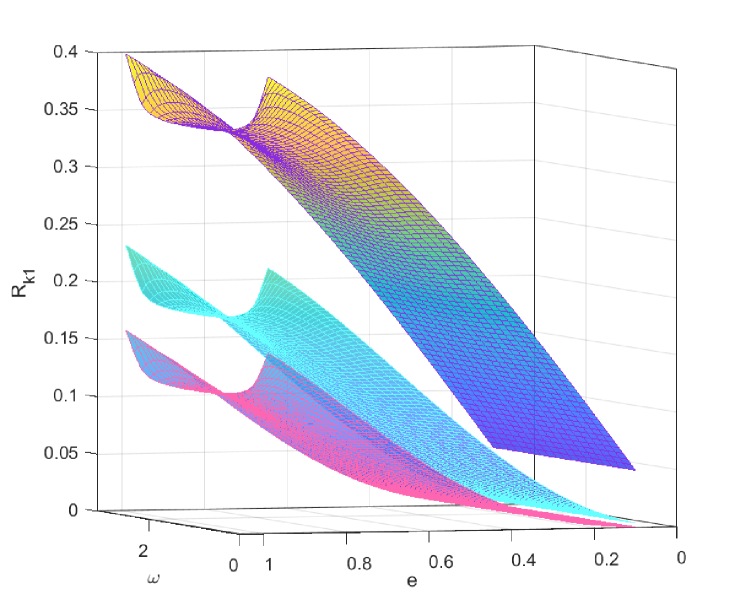
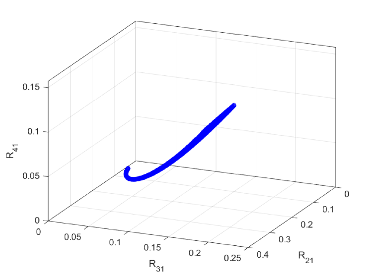
Fig. 2 displays the locus of the points of coordinates , for all and , corresponding to a purely Keplerian LTTE. It can be used in differentiating the LTTE mechanism when compared to other arbitrary periodic phenomena and in determining how close a hypothetical movement is to a Keplerian one [see also Fig. 1 of Pop (1999)].
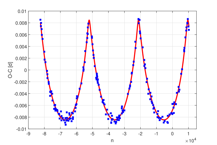
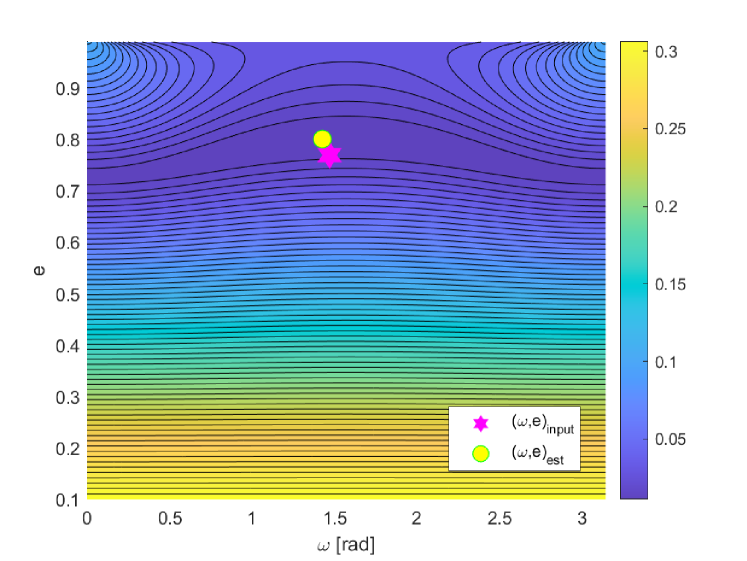
In order to illustrate our approach, we generated a data set of LTTE timing data using the orbital elements for the hypothetical companion of the W UMa type binary system V524 Monocerotis (He et al. 2012; Bulut & Aşkın 2022), superposed on a Gaussian noise with a relatively low standard deviation (see Fig. 3). Due to the fact that the number of the available observed data is relatively small (66), and the orbital cycle coverage is not rich, we increased the number of artificially generated data (200), keeping the same time base. In addition, the data sampling is also irregular and contains random length gaps.
In Fig. 4 we plotted the corresponding objective function, , as given in Eq. (35), for the amplitude ratios for the simulated data set.
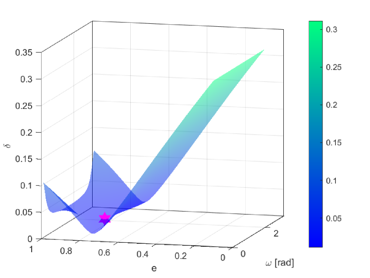
Fig. 5 shows the contour plot of the isolines of the objective function given in Eq. (35) for the simulated LTTE data. As we already mentioned above, for small values of , the objective function is less sensitive to the variation of , while for larger values of , becomes more and more sensitive with respect to (see also Fig. 4).
5 Practical aspects
As previously indicated, in order to consider the investigation of a period variability phenomenon possibly caused by a LTTE, we have to fit a truncated Fourier series to the available timing data. Therefore, it is useful to take into account the run of the respective curve, and also to analyse its amplitude spectrum in order to obtain further information. The following situations may be encountered:
(i) Most frequently the timing data displays time gaps which limits the order of the fitted Fourier series. Thus, according to (a) the local weather conditions experienced by the respective observers, and, sometimes to (b) the historical context (see, e.g., the case of the two World Wars), the available timing data can contain more or less wide time gaps. In order to avoid the oscillation of the fitted curve inside these gaps, a simple condition has to be fulfilled [similar to that proposed by Pop et al. (2004)]: half of the minimum dimensionless period corresponding to the frequency of the highest harmonic which will be taken into account has to be equal to the width of the largest time gap measured in cycle numbers , i.e.,
| (41) |
which becomes
| (42) |
(ii) According to the observational technique and its location (ground or space based), the analysed timing data may contain a more or less amount of additive observational noise.
(iii) In the case of the Fourier expansion of the elliptical motion, the large orbital eccentricity values yield large amplitudes of the higher order harmonics (see Konacki & Maciejewski 1996). On the other hand, according to the level of the observational noise, only (very) low order harmonics can be observed in the amplitude spectrum of the detrended residuals. In case of lower eccentricity orbits, the second harmonic and even the first one may be significantly contaminated by the contribution of the observational noise. As a consequence, by taking too many harmonics, the fitted model will tend to describe the fluctuations caused by the noise. Clearly, in such a situation, the attempt to estimate the values of the orbital elements might be seriously affected.
An elegant solution to this problem may be the use of the Lanczos smoothing factors, already applied by Meylan & Burki (1986) in the case of the radial velocity curves of some pulsating stars. The Lanczos factors are in fact weights which multiply the estimated amplitudes of a truncated Fourier series [see, e.g., Arfken (1970), Hamming (1986)]. For our model, in Eq. (18) they are given by the formula
| (43) |
As it is well-known, these factors have values less than 1 and, for , , which means that the highest harmonic taken into account is completely eliminated. Thus, by reducing the harmonics amplitudes as well as their number, the Lanczos factors perform a smoothing of the Fourier fit. Therefore, a predictable consequence might be an underestimation of the orbital eccentricity value.
References
- Arfken, G. 1970, Mathematical Methods for Physicists, Second Edition, Academic Press, New York
- Borkovits, T., Hegedüs, T.: 1996, A&AS, 120, 63
- Borkovits, T., Rappaport, S., Hajdu, T., Sztakovics, J.: 2015, MNRAS, 448, 946
- Brouwer, D., Clemence, G.M.: 1961, Methods in Celestial Mechanics, Academic Press, New York and London
- Bulut, İ., Aşkın, G.: 2022, New. Astron., 90, 101668 (12 pp.)
- Burki, G., Meylan, G.: 1986, A&A, 156, 131
- De Sitter, A.: 1933, Bull. Astron. Inst. Netherlands, 7, 119
- Esmer, E.M., Baştürk, Ö., Hinse, T.C., Selam, S.O., Correia, A.C.M.: 2021, A&A, 648, id. A85, (22 pp.)
- Hamming, R.W.: 1986, Numerical Methods for Scientists and Engineers, Second Edition, Dover Publications, Inc., New York
- He, J.-J., Wang, J.-J., Qian, S.-B.: 2012, PASJ, 64, 85
- Hinse, T.C., Horner, J., Wittenmyer, R. A.: 2014a, J. Astron. Space. Sci., 31, 187
- Hinse, T.C., Goździewski, K., Lee, J.W., Haghighipour, N., Lee, C.-U.: 2012a, AJ, 144:34 (10 pp.)
- Hinse, T.C., Lee, J. W., Goździewski, K., Haghighipour, N., Lee, C.-U., Scullion, E. M.: 2012b, MNRAS, 420, 3609
- Hinse, T.C., Horner, J., Lee, J.W., Wittenmyer, R.A., Lee, C.-U., Park, J.-H., Marshall, J.P.: 2014b, A&A, 565, A104 (8 pp.)
- Irwin, J.B.: 1952, ApJ, 116, 211
- Irwin, J.B.: 1959, AJ, 64, 149
- Konacki, M., Maciejewski, A.J.: 1996, Icarus, 122, 347
- Konacki, M., Maciejewski, A.J.: 1999, MNRAS, 308, 167
- Kopal, Z.: 1959, Close Binary Systems, Chapman-Hall and John Wiley, London and New York
- Kopal, Z.: 1978, Dynamics of Close Binary Systems, D. Reidel Publishing Company, Dordrecht
- Lee, J.W., Hong, K., Hinse, T.C.: 2015, AJ, 149:93 (7 pp.)
- Lee, J.W., Hinse, T.C., Youn, J.-H., Han, W.: 2014, MNRAS, 445, 2331
- Pop, A.: 1996, Romanian Astron. J., , 6, 147
- Pop, A.: 1998, PhD Thesis, Astronomical Institute of the Romanian Academy, Bucharest
- Pop, A.: 1999, Romanian Astron. J, , 9, 131
- Pop, A.: 2000, Metode de analiză şi interpretare a variabilităţii stelare, Casa Cărţii de Ştiinţă, Cluj-Napoca
- Pop, A., Turcu, V., Codreanu, S.: 2004, Ap&SS, 293, 393
- Pop, A., Crăciun, M., Mocanu, G., Vamoş, C.: 2017, Ap&SS, 362, 76
- Simon, N.R., Lee, A.S.: 1981, ApJ, 248, 291
- Townsend, G.E., Tamburro, M.B.: 1968, Guidance, Flight Mechanics and Trajectory Optimization, Vol. III, The Two-Body Problem, NASA CR-1002, Washington, D.C.
- Woltjer, J.: 1922, Bull. Astron. Inst. Netherlands, 1, 93
[1] Arfken, G. 1970, Mathematical Methods for Physicists, Second Edition, Academic Press, New York Borkovits, T., Hegedus, T.: 1996, Astron. Astrophys. Suppl. , 120, 63
[2] Borkovits, T., Rappaport, S., Hajdu, T., Sztakovics, J.: 2015, Mon. Not. Roy. Astron. Soc. , 448, 946 Brouwer, D., Clemence, G.M.: 1961, Methods in Celestial Mechanics, Academic Press, New York and London
[3] Bulut, I., As¸kın, G., 2022, New. Astron., 90, 101668 (12 pp.)
[4] Burki, G., Meylan, G., 1986, Astron. Astrophys. , 156, 131
[5] De Sitter, A., 1933, Bull. Astron. Inst. Netherlands, 7, 119
[6] Esmer, E.M., Bas¸turk, O., Hinse, T.C., Selam, S.O., Correia, A.C.M.: 2021, Astron. Astrophys. , 648, id. A85, (22 pp.)
[7] Hamming, R.W., 1986, Numerical Methods for Scientists and Engineers, Second Edition, Dover Publications, Inc., New York
[8] He, J.-J., Wang, J.-J., Qian, S.-B., 2012, Pub. Astron. Soc. Japan , 64, 85
[9] Hinse, T.C., Horner, J., Wittenmyer, R. A., 2014a, J. Astron. Space. Sci., 31, 187
[10] Hinse, T.C., Gozdziewski, K., Lee, J.W., Haghighipour, N., Lee, C.-U., 2012a, Astron. J. , 144, 34 (10 pp.)
[11] Hinse, T.C., Lee, J. W., Gozdziewski, K., Haghighipour, N., Lee, C.-U., Scullion, E. M., 2012b, Mon. Not. Roy. Astron. Soc. , 420, 3609
[12] Hinse, T.C., Horner, J., Lee, J.W., Wittenmyer, R.A., Lee, C.-U., Park, J.-H., Marshall, J.P., 2014b, Astron. Astrophys. , 565, A104 (8 pp.)
[13] Irwin, J.B., 1952, Astrophys. J. , 116, 211
[14] Irwin, J.B., 1959, Astron. J. , 64, 149
[15] Konacki, M., Maciejewski, A.J., 1996, Icarus, 122, 347
[16] Konacki, M., Maciejewski, A.J., 1999, Mon. Not. Roy. Astron. Soc. , 308, 167
[17] Kopal, Z., 1959, Close Binary Systems, Chapman-Hall and John Wiley, London and New York
[18] Kopal, Z., 1978, Dynamics of Close Binary Systems, D. Reidel Publishing Company, Dordrecht
[19]Lee, J.W., Hong, K., Hinse, T.C., 2015, Astron. J. , 149:93 (7 pp.)
[20] Lee, J.W., Hinse, T.C., Youn, J.-H., Han, W., 2014, Mon. Not. Roy. Astron. Soc. , 445, 2331
[21] Pop, A., 1996, Romanian Astron. J. , 6, 147
[22] Pop, A., 1998, PhD Thesis, Astronomical Institute of the Romanian Academy, Bucharest
[23] Pop, A., 1999, Romanian Astron. J. , 9, 131
[24] Pop, A., 2000, Metode de analiza si interpretare a variabilitatii stelare, Casa Cartii de Stiinta, Cluj- ˘Napoca
[25] Pop, A., Turcu, V., Codreanu, S., 2004, Astrophys. Space Sci. , 293, 393
[26] Pop, A., Craciun, M., Mocanu, G., Vamos¸, C., 2017, Astrophys. Space Sci. , 362, 76
[27] Simon, N.R., Lee, A.S., 1981, Astrophys. J. , 248, 291
[28] Townsend, G.E., Tamburro, M.B., 1968, Guidance, Flight Mechanics and Trajectory Optimization, Vol. III, The Two-Body Problem, NASA CR-1002, Washington, D.C.
[29] Woltjer, J., 1922, Bull. Astron. Inst. Netherlands, 1, 93