Abstract
The time evolution of a physical quantity associated with a thermodynamic system whose equilibrium fluctuations are modulated in amplitude by a slowly varying phenomenon can be modeled as the product of a Gaussian white noise {Zt} and a stochastic process with strictly positive values {Vt} referred to as volatility.
The probability density function (pdf) of the process Xt=VtZt is a scale mixture of Gaussian white noises expressed as a time average of Gaussian distributions weighted by the pdf of the volatility. The separation of the two components of {Xt} can be achieved by imposing the condition that the absolute values of the estimated white noise be uncorrelated.
We apply this method to the time series of the returns of the daily S&P500 index, which has also been analyzed by means of the superstatistics method that imposes the condition that the estimated white noise be Gaussian. The advantage of our method is that this financial time series is processed without partitioning or removal of the extreme events and the estimated white noise becomes almost Gaussian only as result of the uncorrelation condition.
Authors
Călin Vamoş
Maria Crăciun
Keywords
Paper coordinates
C. Vamoş, M. Crăciun, Separation of components from a scale mixture of Gaussian white noises, Physical Review E, vol. 81 (2010) article id. 051125,
doi: 10.1103/PhysRevE.81.051125
References
see the expansion block below.
soon
About this paper
Print ISSN:
2470-0045
Online ISSN:
2470-0053
Google Scholar profile
google scholar link
Paper (preprint) in HTML form
Separation of components from a scale mixture of Gaussian white noises
Abstract
The time evolution of a physical quantity associated with a thermodynamic system whose equilibrium fluctuations are modulated in amplitude by a slowly varying phenomenon can be modeled as the product of a Gaussian white noise and a stochastic process with strictly positive values referred to as volatility. The probability density function (pdf) of the process is a scale mixture of Gaussian white noises expressed as a time average of Gaussian distributions weighted by the pdf of the volatility. The separation of the two components of can be achieved by imposing the condition that the absolute values of the estimated white noise be uncorrelated. We apply this method to the time series of the returns of the daily S&P500 index, which has also been analyzed by means of the superstatistics method that imposes the condition that the estimated white noise be Gaussian. The advantage of our method is that this financial time series is processed without partitioning or removal of the extreme events and the estimated white noise becomes almost Gaussian only as result of the uncorrelation condition.
PACS:
89.65.Gh, 05.45.Tp, 05.70.LnThere are nonequilibrium thermodynamic systems that for short time periods are in equilibrium states, but their parameters vary over longer time scales. An elementary example of such a system is a Brownian particle moving through a slowly fluctuating environment. If the Brownian particle is always in local equilibrium, then its velocity has a Gaussian distribution with slowly varying parameters. The average global velocity distribution is a superposition of Gaussians weighted by the probability density of the slowly fluctuating parameters. Depending on the type of the statistical distribution of the slow fluctuations of the environment, the particle velocity may have different types of statistical distributions named superstatistics beck03 .
A time series obtained by measuring a thermodynamic system with superstatistics can be modeled as the product of two stochastic processes
| (1) |
where and and are independent. The Gaussian white noise models the equilibrium thermodynamic fluctuations, while the stochastic process with strictly positive values describes the slow fluctuations of the environment. If is not only uncorrelated, but independent and identically distributed (i.i.d.), then is called heteroskedastic. We emphasize that the independence of and does not preclude the dependence of on the preceding terms and , , as for example, in the ARCH and GARCH models engle82 ; boller86 .
Although the financial markets are not usual thermodynamic systems, many of the methods in statistical physics can be applied to such complex social phenomena voit05 . For a financial time series the white noise in the heteroskedastic process (1) models the efficiency of the financial markets, i.e., the uncorrelation of successive price variations. The significant long-range correlations of the absolute values of the price fluctuations are due to the slowly varying stochastic process , which modulates the amplitude of the white noise fluctuations. As in finance, we name it volatility.
A numerical method to estimate the two factors in Eq. (1) is the partitioning of the time series into slices for which the thermodynamic local equilibrium holds straet09 . The partitioning is achieved by imposing the condition that the mean kurtoses of over the slices equal the Gaussian kurtosis. The superstatistics method has been applied to a variety of complex systems with time scale separation in turbulence, share price fluctuations, cosmic rays, traffic delays, metastasis and cancer survival, etc. beck09 . Because the normality is tested by means of the fourth moment, the superstatistics method is sensitive to the presence of outliers. For example, it was necessary to eliminate the extreme events from some financial time series in order to analyze them straet09 . A similar approach for intraday returns is presented in gerig09 . The main difference is that the slices length is predetermined to a day and the volatility is considered constant over intraday time scales.
The equilibrium thermodynamic fluctuations are not only Gaussian, but also independent, and, consequently, uncorrelated. Hence the separation of the components of the stochastic process (1) can be obtained by imposing instead of the normality condition, the condition that the absolute values of the estimated noise be uncorrelated. The question is about the relation between these two conditions, i.e., if we impose one condition, then to what degree is the other condition also satisfied. In this Rapid Communication we show that by imposing the uncorrelation condition, the estimated white noise becomes almost Gaussian, proving that it entails the normality condition.
Our results indicate that the uncorrelation condition is numerically more efficient than the normality one. We apply this method to the time series of the daily S&P500 index analyzed in straet09 , without its partitioning and without eliminating any extreme value. It is possible that this greater efficiency be due to a more complete exploitation of the temporal variation of all the observed values, not only the variation from one slice to the other.
Although the physical systems modeled by Eq. (1) are normal in the conventional thermodynamic sense, they seem anomalous by featuring non-Gaussian statistics. If the volatility is stationary, then is also stationary and its probability density function (pdf) is a scale mixture of normal distributions given by the integral
| (2) |
where is the pdf of andrews74 . According to this formula, is the result of the superposition of Gaussians whose standard deviations are realizations of the volatility , that is why we say that is the mixture of Gaussians with scales distributed according to . A large class of systems with polydisperse features has the pdf with power-law tails as a result of the superposition of Gaussians with the variances obeying a gamma distribution gherghiu04 .
A direct generalization of the scale mixture of normal distributions is obtained if the volatility is nonstationary. Since in Eq. (2) explicitly depends on time, then also varies in time. The global average pdf is the time average of
and we refer to it as a scale mixture of Gaussian white noises. This distinct denomination emphasizes the importance of the time dependence of the volatility which allows for a greater range of shapes for the pdfs than Eq. (2). In this case the volatility can describe a deterministic variation imposed by the environment on the measured system or a superposition of a stationary random fluctuations on such a deterministic evolution.
We determine the white noise by first estimating the volatility by one of the two main methods in quantitative finance poon05 . The first method expresses the volatility by the explicit relations that define stochastic models of the financial time series. The second method is based on the averaging of historical values of the absolute or square returns at a high enough sampling frequency. Such estimators are called “realized volatility” and it is shown that for continuous stochastic processes they are unbiased estimators andersen02 . In practice various types of averaging are used. The best known is the exponential weighted moving average of the Riskmetrics model riskmetr96 . The daily volatility is also often estimated by averaging the intraday data andersen98 . In this paper we estimate the volatility by means of a modified form of the moving average presented in liu99 and we find the optimum moving average using the uncorrelation condition.
We consider a time series as a finite realization of the stochastic process . We follow the practice of denoting by small letters the realizations of the stochastic processes denoted by the corresponding capitals. In this way we keep clear the distinction between the different nature of a stochastic process (family of measurable functions defined on a probability space) and one of its realizations which is a series of real numbers equal with the values taken by the measurable functions at particular events. In fact the stochastic process does not model the time series, but the random phenomenon which is assumed to generate the observed time series.
If is the semilength of the averaging window, then for we define the moving average
| (3) |
If (), then the average is taken over the first (the last ) values of . This asymmetric average forces the values near the time series boundaries to follow the variations of the interior values. If we consider as a volatility estimator, then from Eq. (1) it follows that the estimator of the white noise is
| (4) |
We have to find the optimum value satisfying the condition that the series be uncorrelated. This condition cannot be imposed to the signed series since, like the initial time series , it is uncorrelated. This property results from the randomness of the sign variations of the white noise in Eq. (1), which is preserved by multiplication with the strictly positive values of the slowly varying volatility .
The sample autocorrelation function (ACF) of an uncorrelated infinite time series is identical zero. Bartlett’s formula states that for a finite i.i.d. Gaussian process, the pdf of the sample ACF is Gaussian with mean and variance , where is the length of the time series brockdav96 . The proof presented in brockdav96 can be reproduced with minimal changes for the absolute values of an i.i.d. Gaussian process and it follows that Bartlett’s formula holds in this case too.
We measure the deviation from normality of the sample ACF of the time series , denoted , by the statistic used in the Kolmogorov-Smirnov test
| (5) |
where is the sample cumulative distribution function (cdf) of and is the theoretical cdf of the normal distribution with Bartlett’s parameters. The quantity is an index measuring the nonnormality of , i.e., the serial correlation of . If is the value for which is minimum, then the volatility estimator is and from Eq. (4) it follows that the estimator of the white noise is .
We test this algorithm on the daily S&P500 index studied in straet09 on which several scaling analyses have been performed liu99 ; Gopi99 ; mantegna95 . It has also been proved by a statistical analysis that this time series can be modeled as the product of the volatility and an i.i.d. stochastic process starica05 . This conclusion is in accordance with the heteroskedastic decomposition in Eq. (1) on which all the volatility stochastic models are build poon05 . Its validity is sustained also by the results analogous to those for the S&P500 index obtained with the uncorrelation condition for several stock market indices (Dow Jones, Nikkei, FTSE, etc.) and several large cap stocks (INTC, MSFT, IBM, MRK, etc.).
We examine the S&P500 index in the interval between January 1st, 1950 and December 31st, 2009 containing trading days. If we denote by the daily closing values of the S&P500 index, then the logreturn over the temporal interval is defined as
For the logreturns are computed only for , otherwise the temporal intervals would overlap each other and spurious correlations would occur between the logreturns. Also, the mean is extracted from the final time series .
We suppose that, for a given , the time series is a finite sample of an infinite discrete stochastic process of the form of Eq. (1). The average (3) is performed only on the daily logreturns (), so that the information at the highest available frequency is used even if we estimate the volatility for . This choice is in agreement with the theoretical result that the realized volatility is closer to the real one if data frequency is increased andersen02 .
The index defined by Eq. (5) depends on two parameters ( and ). The choice of the number of sample ACF values is a difficult problem with no simple solution escan09 . As a general rule should be smaller than a quarter of the time series length box94 . However, the sample ACF is different from that of a white noise especially for the small values of . Moreover, if the serial correlation for small is reduced, then the entire ACF becomes negligible. As a consequence, we limit the value of in Eq. (5) only to several tens.
In Fig. 1(a) we present the variation of the index for with respect to the semilength of the averaging window for several values of . Each curve has two minima. The first minimum corresponds to an averaging with , which does not significantly damp the fluctuations of the logreturns, so that the average preserves these fluctuations. We are interested in the second minimum occurring when for which the average is slowly varying. For other values of the first minimum is greater than the second one or even does not exist and then the minimum supplying the estimated volatility coincides with the global minimum.
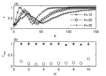
The minimum values of the index for which the white noise is estimated are compared in Fig. 1(b) with which is the index computed for the initial logreturns time series. The minimum of is obtained by exhaustive search for and . One notices that for all time scales , is close to 1, indicating that all the values of the sample ACF implied in the computation of lay outside the variation range of the ACF of a white noise. The values of are significantly smaller than the corresponding showing that the estimated white noise is much closer to an uncorrelated time series than the initial logreturns.
In order to verify that the uncorrelation condition entails the normality of the estimated white noise, we compute the Kolmogorov-Smirnov statistic of . In comparison with Eq. (5) the difference is that is the cdf of the normalized estimated white noise, not of its sample ACF, and is the cdf of a normalized Gaussian. Figure 2 shows the values of for compared with those for the normalized initial logreturns . It also contains the mean and the standard deviation of for statistical ensembles of 1000 numerically generated i.i.d. Gaussian time series having the same length as of S&P500. The results show that the estimated white noise has a probability distribution much closer to a Gaussian than that of the initial logreturns. One notices that for it cannot be differentiated from an i.i.d. Gaussian time series.
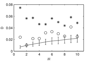
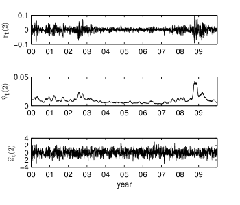
Figure 3 shows the logreturns, the estimated volatility, and the estimated white noise after the year 2000 for . The increased variability of the logreturns amplitude (volatility clustering) is no more present in the estimated white noise. Even the most volatile period of the financial crisis which started in 2008 is correctly described by the estimated volatility. We have obtained this result without removing any extreme value from the logreturns as it is necessary in the superstatistics method straet09 .
In order to test the separation algorithm in its simplest form, we have processed the entire logreturns time series, without any partitioning. However, for such a long time series () it is possible that the search for the minimum of the index be more efficient over shorter fragments. Then the white noise obtained by joining the white noises estimated over shorter segments could be more similar to an uncorrelated time series. The partitioning of a nonstationary time series might be obtained by existing algorithms Fukuda04 .
The method presented in this paper numerically separates the two components of a scale mixture of Gaussian white noises and it can be applied to many phenomena characterized by the modulation in amplitude of the thermodynamic equilibrium fluctuations by a slowly varying process. Such phenomena are those already studied by means of the superstatistics method: turbulence, share price fluctuations, cosmic rays, traffic delays, metastasis and cancer survival, etc. beck09 . Some biophysical processes, for example, the human heart rate fluctuations, also present these features Galvan01 .
If the white noise does not have a Gaussian distribution, Bartlett’s formula has to be modified for each type of pdf. For instance, at time scales of minutes the logreturns have a two-tailed exponential distribution Silva04 . In such cases the separation of the components using the uncorrelation condition gives different results depending on the assumed type of the probability distribution of the white noise. The choice of the correct pdf might be possible by means of the resemblance degree between the pdf of the estimated noise and the one that was initially assumed.
References
- (1) C. Beck and E.G.D. Cohen, Physica A 322, 267 (2003).
- (2) R.F. Engle, Econometrica 50, 987 (1982).
- (3) T. Bollerslev, J. Econometrics 31, 307 (1986).
- (4) J. Voit, The Statistical Mechanics of Financial Markets, 3rd ed. (Springer, Berlin, 2005).
- (5) E. Van der Straeten and C. Beck, Phys. Rev. E 80, 036108 (2009).
- (6) C. Beck, Braz. J. Phys. 39, 357 (2009).
- (7) A. Gerig, J. Vicente, and M.A. Fuentes, Phys. Rev. E 80, 065102(R) (2009).
- (8) D.F. Andrews and C.L. Mallows, J. Roy. Stat. Soc. B 36, 99 (1974).
- (9) S. Gheorghiu and M.-O. Coppens, PNAS 101, 15852 (2004).
- (10) S.-H. Poon, A Practical Guide to Forecasting Financial Market Volatility (Wiley Finance, 2005).
- (11) T.G. Andersen, T. Bollerslev, and F.X. Diebold, NBER Technical Working Paper No. 279, 2002.
- (12) J. Longerstaey and P. Zangari, RiskMetrics-Technical Document, 4th ed. (Morgan Guaranty Trust Co., New York, 1996).
- (13) T.G. Andersen and T. Bollerslev, Int. Econ. Rev. 39, 85 (1998).
- (14) Y. Liu, P. Gopikrishnan, P. Cizeau, M. Meyer, C.-K. Peng, and H.E. Stanley, Phys. Rev. E 60, 1390 (1999).
- (15) P.J. Brockwell and R.A. Davies, Time Series: Theory and Methods, (Springer Verlag, New York, 1996).
- (16) P. Gopikrishnan, V. Plerou, L.A. Nunes Amaral, M. Meyer, and H.E. Stanley, Phys. Rev. E 60, 5305 (1999).
- (17) R.N. Mantegna and H.E. Stanley, Nature 376, 46 (1995).
- (18) C. Stărică and C. Granger, Rev. Econ. Stat. 87, 503 (2005).
- (19) J.C. Escanciano and I.N. Lobato, J. Econometrics 151, 140 (2009).
- (20) G. Box, G. Jenkins and G. Reinsel, Time series analysis: Forecasting and control, 3rd ed. (Prentice-Hall, Upper Saddle River, NJ, 1994).
- (21) K. Fukuda, H.E. Stanley, and L.A. Nunes Amaral, Phys. Rev. E 69, 021108 (2004).
- (22) P. Bernaola-Galván, P.C. Ivanov, L.A. Nunes Amaral, and H.E. Stanley, Phys. Rev. Lett. 87, 168105 (2001).
- (23) A.C. Silva, R.E. Prange, and V.M. Yakovenko, Physica A 344, 227 (2004); H. Kleinert and X.J. Chen, Physica A 383, 513 (2007)
[1] C. Beck and E. G. D. Cohen, Physica A 322, 267 2003.
[2] R. F. Engle, Econometrica 50, 987 1982.
[3] T. Bollerslev, J. Econometrics 31, 307 1986.
[4] J. Voit, The Statistical Mechanics of Financial Markets, 3rd ed. Springer, Berlin, 2005.
[5] E. Van der Straeten and C. Beck, Phys. Rev. E 80, 036108 2009.
[6] C. Beck, Braz. J. Phys. 39, 357 2009.
[7] A. Gerig, J. Vicente, and M. A. Fuentes, Phys. Rev. E 80, 065102R 2009.
[8] D. F. Andrews and C. L. Mallows, J. R. Stat. Soc. Ser. B Methodol. 36, 99 1974.
[9] S. Gheorghiu and M.-O. Coppens, Proc. Natl. Acad. Sci. U.S.A. 101, 15852 2004.
[10] S.-H. Poon, A Practical Guide to Forecasting Financial Market Volatility Wiley Finance, Chichester, 2005.
[11] T. G. Andersen, T. Bollerslev, and F. X. Diebold, NBER Technical Working Paper No. 279, 2002 unpublished.
[12] J. Longerstaey and P. Zangari, Risk Metrics—Technical Document, 4th ed. Morgan Guaranty Trust Co., New York, 1996.
[13] T. G. Andersen and T. Bollerslev, Int. Econom. Rev. 39, 885 1998.
[14] Y. Liu, P. Gopikrishnan, P. Cizeau, M. Meyer, C.-K. Peng, and H. E. Stanley, Phys. Rev. E 60, 1390 1999.
[15] P. J. Brockwell and R. A. Davies, Time Series: Theory and Methods Springer Verlag, New York, 1996.
[16] P. Gopikrishnan, V. Plerou, L. A. Nunes Amaral, M. Meyer, and H. E. Stanley, Phys. Rev. E 60, 5305 1999.
[17] R. N. Mantegna and H. E. Stanley, Nature London 376, 46 1995.
[18] C. Stărică and C. Granger, Rev. Econ. Stat. 87, 503 2005.
[19] J. C. Escanciano and I. N. Lobato, J. Econometrics 151, 140 2009.
[20] G. Box, G. Jenkins, and G. Reinsel, Time Series Analysis: Forecasting and Control, 3rd ed. Prentice-Hall, Upper Saddle River, NJ, 1994.
[21] K. Fukuda, H. E. Stanley, and L. A. Nunes Amaral, Phys. Rev. E 69, 021108 2004.
[22] P. Bernaola-Galván, P. Ch. Ivanov, L. A. Nunes Amaral, and H. E. Stanley, Phys. Rev. Lett. 87, 168105 2001.
[23] A. C. Silva, R. E. Prange, and V. M. Yakovenko, Physica A 344, 227 2004; H. Kleinert and X. J. Chen, ibid. 383, 513 2007.