Abstract
In this paper we solve by method of lines (MoL) a class of pseudo-parabolic PDEs defined on the real line. The method is based on the sinc collocation (SiC) in order to discretize the spatial derivatives as well as to incorporate the asymptotic behavior of solution at infinity. This MoL casts an initial value problem attached to these equations into a stiff semi-discrete system of ODEs with mass matrix independent of time. A TR-BDF2 finite difference scheme is then used in order to march in time.
The method does not truncate arbitrarily the unbounded domain to a finite one and does not assume the periodicity. These are two omnipresent, but non-natural, ingredients used to handle such problems. The linear stability of MoL is proved using the pseudospectrum of the discrete linearized operator.
Some numerical experiments are carried out along with an estimation of the accuracy in conserving two invariants. They underline the efficiency and robustness of the method. The convergence order of MoL is also established.
Authors
Keywords
References
See the expanding block below.
Paper coordinates
C.I. Gheorghiu, Spectral Collocation Solutions to a Class of Pseudo-parabolic Equations, G.Nikolov et al. (Eds.): NMA 2018, LNCS 11189, pp. 1-8, 2019, doi: 10.1007/978-3-030-10692-8_20
About this paper
Journal
Springer
Publisher Name
Numerical Methods and Applications
DOI
10.1007/978-3-030-10692-8_20
Print ISSN
?
Online ISSN
?
Google Scholar Profile
aici se introduce link spre google scholar
Paper (preprint) in HTML form
Spectral Collocation Solutions to a Class of Pseudo-Parabolic Equations.††thanks: Partly supported by organization UEFISCDI MC2018.
Abstract
In this paper we solve by method of lines (MoL) a class of pseudo-parabolic PDEs defined on the real line. The method is based on the sinc collocation (SiC) in order to discretize the spatial derivatives as well as to incorporate the asymptotic behavior of solution at infinity. This MoL casts an initial value problem attached to these equations into a stiff semi-discrete system of ODEs with mass matrix independent of time. A TR-BDF2 finite difference scheme is then used in order to march in time.
The method does not truncate arbitrarily the unbounded domain to a finite one and does not assume the periodicity. These are two omnipresent, but non-natural, ingredients used to handle such problems.
The linear stability of MoL is proved using the pseudospectrum of the discrete linearized operator. Some numerical experiments are carried out along with an estimation of the accuracy in conserving two invariants. They underline the efficiency and robustness of the method. The convergence order of MoL is also established.
Keywords:
pseudo-parabolic equation infinite domain Camassa-Holm peakon sinc collocation TR-BDF2 linear stability pseudospectrum.1 Camassa-Holm Equation
Camassa and Holm [4] introduce the equation,
| (1) |
discuss its analytical properties and sketch its derivation. Here is the fluid velocity in the direction, is a constant related to the critical shallow-water wave speed, and subscripts denote partial derivatives.
Actually, the equation is a new completely integrable dispersive shallow water equation that is bi-Hamiltonian. For the authors quoted above showed that this equation has solitary water waves of the form which they called ”peakons”. Dropping both high-order terms from the r. h. s. of (1) leads to the familiar Benjamin-Bona-Mahony (BBM) equation [2], or at the same order, to the Korteweg-de Vries (KdV) equation. Nevertheless, these extra terms profoundly alter the behavior of solitary waves. Thus, this extension of the BBM equation possesses soliton solutions whose limiting forms as have peaks where first derivatives are discontinuous, i.e. peakons. The lack of smoothness at the peak of the peakon introduces high-frequency dispersive errors into the calculation. This is one of the main numerical challenges.
There is a fairly rich literature gathered around the Camassa-Holm equation. For instance, in [3] J. P. Boyd derives a perturbation series solution for general which converges even at peakon limit and also gives three analytical formulations for spatially representations of the peakons. He also observes that although the Camassa-Holm equation is integrable for general , it appears that imbricating solitary waves generates an exact spatially periodic solution only for the special cases and . Camassa, Holm and Hyman [5] present periodic numerical solutions to equation (1) and a large discussion to this equation as a Hamiltonian system. They focus on the case . Actually, we also have some performing methods, like Runge-Kutta discontinuous Galerkin, for periodic case or bounded domains obtained by empiric truncation.
The main motivation to design this MoL-SiC scheme is to avoid the arbitrary truncation of the domain or periodicity assumptions. Instead, we suggest an asymptotic truncation of the integration domain through the scaling factor of SiC. The present paper provides accurate numerical results for arbitrary case. We use a MoL based on SiC in order to discretize the spatial derivatives and TR-BDF2 in order to march in time.
The boundary conditions for solution will be taken to be regular at infinity, i.e.
| (2) |
for at least where denotes the derivative with respect to . They are here behavioral (natural) rather than numerical and have been inspired by the analysis in [2].
The pure initial-value problem for the above equation is to ask for a solution defined for having a specified initial configuration namely
| (3) |
A typical situation arises wherein the initial disturbance has sensibly finite extent. Thus, we suppose a datum being drawn from some classes of functions having limit at , i.e., satisfying at least the first condition in (2). In such circumstances the pure initial value problem for (1) is well-posed in Hadamard’s classical sense (see [1]). That is, corresponding to a suitable initial datum , there is a unique function defined on satisfying the differential equation there, and for which (2) holds. Moreover, if is slightly perturbed in its function class, then the solution changes only slightly in response.
2 MoL Discretization to Camassa-Holm Equation
The MoL solution to the equation (1) reads
| (4) |
where are the sinc discrete functions introduced and analyzed by F. Stenger in [10] and for are the nodal time unknowns. is the order of approximation.
The functions are defined by
where are the equispaced nodes with spacing , symmetric with respect to the origin and .
It is important to observe that SiC approximation defined by (4) satisfies the regularity condition at infinity (2). The sinc differentiation collocation matrices on are denoted by , . In order to implement the MoL we have used the form of these matrices provided by Weideman and Reddy in [12].
The Camassa-Holm PDE is one of the form
| (5) |
where the operators and are linear and is a nonlinear one. Once we discretize the spatial part of this PDE we get a system of ODEs,
| (6) |
where the vector is defined by
The particular form of the discrete formulation (6) for Camassa-Holm equation reads
| (7) |
where the dot, as in MATLAB, signifies the element wise product of two vectors.
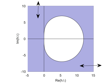
For our dispersive problem it is known that the eigenvalues of the linear operator are close to the imaginary axis (see the analysis in [9]). They are depicted in Fig. 2 and are situated inside or very close to the region of stability of TR-BDF2 depicted in Fig. 1. This is the main reason in choosing this finite difference scheme to solve the ODEs system (7).
3 Linear Stability of MoL
We adopt the strategy from [11] in order to establish the linear (numerical) stability of MoL. We have successfully used this strategy in our contribution [7] in solving numerically the BBM equation which is another pseudo-parabolic one. The linearization of the discrete equation (7) is simply
| (8) |
where is the unit matrix of order . Its pseudospectrum is depicted in Fig. 2 and shows that indeed all eigenvalues are on the imaginary axis.
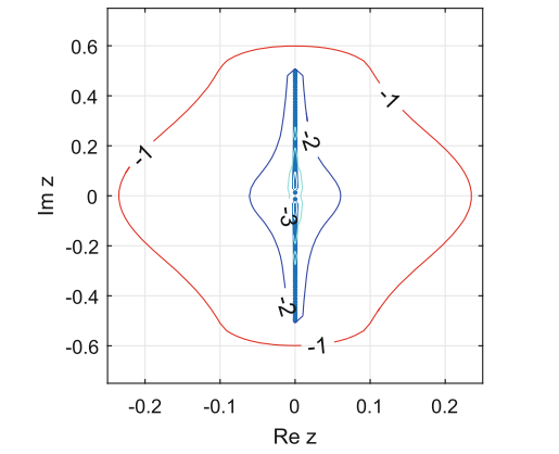
If we overlap Fig. 2 and the region of stability of TR-BDF2 from Fig. 1 we observe the -pseudospectrum lies within a distance + of the stability region as and . Typically the time step has been of order when (1) has been solved.
Thus we can conclude that the MoL-SiC scheme along with TR-BDF2 is numerically stable irrespective of values of parameter . In fact, our numerical experiments have provided reasonable numerical results for the case even if the above analysis of stability does not literally apply to this case.
4 Numerical Experiments
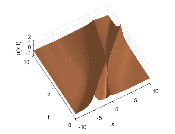
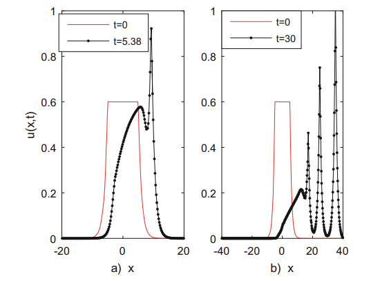
Some numerical experiments will be reported in this section. We consider the interaction of two peakons which emerge from the initial data
| (9) |
Actually we solve the Cauchy’s problem (1)-(9). The interaction of two peakons as singular soliton solutions is depicted in Fig. 3.
The evolution of initial data (9) to its final form of two separated and reversed in order peakons is provided in Fig. 4.
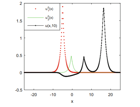
These solitons travel with a speed proportional to their height and remain coherent after their collision (a short animation is instructive in this respect). In spite of the fact that peakons are nonanalytic solitons, a careful inspection of Fig. 3 and Fig. 4 shows that no oscillations (like Gibbs’ ones) appear when resolving the cusp of peakons.
4.1 The Accuracy of MoL
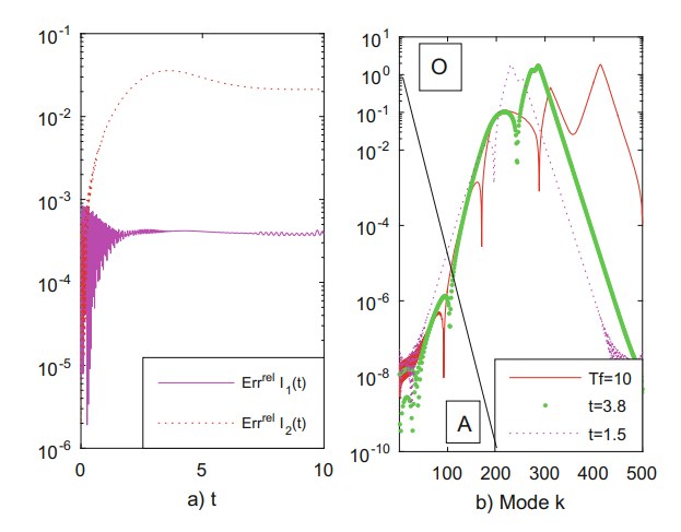
We are now concerned with the accuracy of our outcomes (see also our contribution [8], Sect. 2.1). Thus in a log-linear plot we display in the b) panel of Fig. 5 the absolute values of the coefficients of SiC solutions at several time moments.
We recall an important aspect of SiC, namely the formulation of the collocation and the Galerkin methods for a boundary value problem using sinc functions is perfectly synonymous. Consequently, two important conclusions can be inferred from this figure. First, as time proceed the computations are carried out with the same accuracy. Second, from the same right panel b), we observe that the coefficients behave like with which means the coefficients of SiC solution decrease only exponentially rather than super exponentially (which requires ) as time proceed.
Constantin and Strauss [6] give a very simple proof of the orbital stability of the peakons in the norm using the following two conservation laws
| (10) |
Now we can be more precise and call a solution to (1) if is a solution to (1)-(3) in the sense of distributions and and are conserved for . We will use these conservation laws in order to asses the accuracy of our outcomes. We now introduce the relative errors for the invariants and with
| (11) |
and display them in the left panel of Fig. 5. Corresponding to the initial data (9) we have and . Moreover, the value in (11) stands for the number of integration steps used by TR-BDF2. We carry out the integration in (10) using a trapezoidal quadrature between the extreme nodes in SiC grid. In order to validate once more the above MoL we solve equation (1) with the initial data
| (12) |
The solution is depicted in Fig. 6 and is in perfect accordance with well established results.
5 Concluding Remarks
The MoL-SiC along with TR-BDF2 proved to be a reliable and effective method to solve some Cauchy’s problems attached to a pseudo-parabolic equation. The computational effort is kept in fairly reasonable limits, i.e., some seconds in order to solve the system of semi-discrete ODEs on a usual machine.
The linear stability of MoL is established but a nonlinear one is an open problem. The conservation of two invariants is kept in reasonable limits during the time integration interval. The first one behaves better than the second as expected. Moreover, with respect to the accuracy of method we establish that the convergence is only exponentially.
References
- [1] Amick, C.J., Bona, J.L., Schonbek, M.E.: Decay of Solutions of Some Nonlinear Wave Equations. J. Differ. Equations 81, 1–49 (1989). doi:10.1016/0022-0396(89)90176-9
- [2] Benjamin, T.B., Bona, J.L., Mahony, J.J.: Model Equations for Long Waves in Nonlinear Dispersive Systems. Philos. Trans. Roy. Soc. London Ser.A. 272, 47–78 (1972). doi:10.1098/rsta.1972.0032
- [3] Boyd, J.P.: Peakons and Coshoidal Waves: Traveling Wave Solutions of the Camassa-Holm Equation. Appl. Math. Comput. 81, 173–187 (1997). doi:10.1016/0096-3003(95)00326-6
- [4] Camassa, R., Holm, D.D.: An Integrable Shallow Water Equation with Peaked Solitons. Phys. Rev. Lett. 71, 1661–1664 (1993). doi:10.1103/PhysRevLett.71.1661
- [5] Camassa, R., Holm, D.D., Hyman, J.M.:A New Integrable Shallow Water Equation. In T.-Y. Wu, J. W. Hutchinson. (eds.) vol. 31, pp. 1-31. Academic (1994)
- [6] Constantin, A., Strauss, A.W.: Stability of Peakons. Commun. Pure Appl. Math. 53, 603–-10 (2000). doi:10.1002/(SICI)1097-0312(200005)53:5603::AID-CPA33.0.CO;2-L
- [7] Gheorghiu, C.I.: Stable spectral collocation solutions to a class of Benjamin Bona Mahony initial value problems. Appl. Math. Comput. 273, 1090–1099 (2016). doi: 10.1016/j.amc.2015.10.078
- [8] Gheorghiu, C.I.: Spectral Collocation Solutions to Problems on Unbounded Domains. Casa Cărţii de Ştiinţă Publishing House, Cluj-Napoca (2018)
- [9] Kassam, A.-K., Trefethen, L.N.: Fourth-Order Time-Stepping for Stiff PDEs. SIAM J. Sci. Comput. 26, 1214–-1233 (2005). doi:10.1137/S1064827502410633
- [10] Stenger, F.: Summary of sinc numerical methods. J. Comput. Appl. Math. 121, 379–420 (2000). doi:10.1016/S0377-0427(00)00348-4
- [11] Trefethen, L.N.: Spectral Methods in MATLAB. SIAM Philadelphia (2000)
- [12] Weideman, J.A.C., Reddy, S. C.: A MATLAB Differentiation Matrix Suite. ACM T. Math. Software. 26, 465–519 (2000). doi:10.1145/365723.365727
[1] Amick, C.J., Bona, J.L., Schonbek, M.E., Decay of solutions of some nonlinear wave equations. J. Differ. Equations 81, 1–49 (1989).
[2] Benjamin, T.B., Bona, J.L., Mahony, J.J., Model equations for long waves in nonlinear dispersive systems. Philos. Trans. Roy. Soc. Lond. Ser.A. 272, 47–78 (1972).
[3] Boyd, J.P., Peakons and coshoidal waves: traveling wave solutions of the Camassa-Holm equation. Appl. Math. Comput. 81, 173–187 (1997).
[4] Camassa, R., Holm, D.D., An integrable shallow water equation with peaked solitons. Phys. Rev. Lett. 71, 1661–1664 (1993).
[5] Camassa, R., Holm, D.D., Hyman, J.M., A new integrable shallow water equation. In: Wu, T.-Y., Hutchinson, J.W. (eds.) Advances in Applied Mechanics, vol. 31, pp. 1–31. Academic Press, New York (1994)Google Scholar
[6] Constantin, A., Strauss, A.W., Stability of Peakons. Commun. Pure Appl. Math. 53, 603–610 (2000). 10.1002/(SICI)1097-0312(200005)53:5<<603::AID-CPA3>>3.0.CO;2-L
[7] Gheorghiu, C.I., Stable spectral collocation solutions to a class of Benjamin Bona Mahony initial value problems. Appl. Math. Comput. 273, 1090–1099 (2016).
[8] Gheorghiu, C.I., Spectral Collocation Solutions to Problems on Unbounded Domains. Casa Cărţii de Ştiinţă Publishing House, Cluj-Napoca (2018)
[9] Kassam, A.-K., Trefethen, L.N., Fourth-order time-stepping for stiff PDEs. SIAM J. Sci. Comput. 26, 1214–1233 (2005).
[10] Stenger, F., Summary of sinc numerical methods. J. Comput. Appl. Math. 121, 379–420 (2000).
[11] Trefethen, L.N., Spectral Methods in MATLAB. SIAM Philadelphia (2000)
[12] Weideman, J.A.C., Reddy, S.C., . ACM T. Math. Softw. 26, 465–519 (2000).