A survey on the high convergence orders and computational convergence orders of sequences

6 years ago

(survey), Convergence order, history, ISI/JCR, Numerical Analysis, paper

This is the first paper which surveys the rigorous definitions and relations of convergence orders (the Q-orders; the C-orders; the R-orders) of convergent sequences, and the computational variants.

Abstract

Let $x_k\rightarrow x^\ast\in{\mathbb R}^N$; denote the errors by $ e_k: = \|x^\ast – x_k\| $ and the quotient factors by $Q_p(k)=\frac{e_{k+1}}{{e_k}^p}$ ($p \geq 1$).

Consider the following definitions of Q-orders $p_0>1$ of $\{x_k\}$:

\begin{equation}\tag{$Q_\varepsilon$}\label{def Qe}
\begin{cases}
Q_p=0, & p \in [1,p_0),
\\
Q_p=+\infty, & p \in (p_0,+\infty)
\end{cases}
\Leftrightarrow
\begin{cases}
Q_{p_0-\varepsilon}=0, & \forall \varepsilon >0, p_0-\varepsilon>1,
\\
Q_{p_0+\varepsilon}=+\infty, & \forall \varepsilon >0
\end{cases}
\end{equation}

\begin{equation}\tag{$Q$}\label{def Q}
q_l=q_u, {\rm where}
\begin{cases}
q_l=\inf \big\{p\in[1,+\infty) : \bar{Q}_p=+\infty\big\}, \quad \bar{Q}_p=\limsup\limits_{k\rightarrow\infty}Q(k)
\\
q_u=\sup \big\{p\in[1,+\infty) : \underset{\bar{}}{Q}{}_p=0\big\}, \quad \underset{\bar{}}{Q}{}_p=\liminf\limits_{k\rightarrow\infty}Q(k)
\end{cases}
\end{equation}

\begin{equation}\tag{$Q_L$}\label{def Q_L}
\lim\limits_{k\rightarrow \infty}
\frac{\ln e_{k+1}}{\ln e_k}=p_0
\end{equation}

$\forall \varepsilon>0, \exists A,B\geq 0, \ k_0 \geq 0$ s.t.
\begin{equation}\tag{$Q_{I,\varepsilon}$}\label{f. def Q_eps}
A\cdot e_k ^{p_{0}+\varepsilon}\leq e_{k+1} \leq B\cdot e_k^{p_{0}-\varepsilon},\ \; \; \forall k\geq k_0
\end{equation}

\begin{equation}\tag{$Q_\Lambda$}\label{def Q_Lam}
\lim\limits_{k\rightarrow \infty}
\frac{\ln \frac{e_{k+2}}{e_{k+1}}}{\ln \frac{e_{k+1}}{e_k}}=p_0.
\end{equation}

Twenty years after the classical book of Ortega and Rheinboldt was published, the above definitions for the Q-orders were independently and rigorously studied (i.e., some orders characterized in terms of others), by Potra (1989), resp. Beyer, Ebanks and Qualls (1990). The relationship between all the five definitions (only partially analyzed in each of the two papers) was not subsequently followed and, moreover, the second paper slept from the readers attention.

The main aim of this paper is to provide a rigorous, selfcontained, and, as much as possible, a comprehensive picture of the theoretical aspects of this topic, as the current literature has taken away the credit from authors who obtained important results long ago.

Authors

Emil Cătinaş
(Tiberiu Popoviciu Institute of Numerical Analysis, Romanian Academy)

Keywords

Convergent sequences in $\mathbb{R}^n$; (Q)-convergence orders; (C)-convergence orders; (R)-convergence orders; convergence rates; rates of convergence; convergence speed; speed of convergence; computational convergence orders.

Cite this paper as

E. Cătinaş, A survey on the high convergence orders and computational convergence orders of sequences, Appl. Math. Comput., 343 (2019) 1-20.
doi: 10.1016/j.amc.2018.08.006

PDF

http://doi.org/10.1016/j.amc.2018.08.006

About this paper

Journal

Applied Mathematics and Computation

Publisher Name

Elsevier

DOI

10.1016/j.amc.2018.08.006

Print ISSN

0096-3003

Online ISSN

Google Scholar citations

google scholar citations

Errata

The sequence $z_k$ from Example 2.8 actually does not have Q-order $2$:
\[
z_k = \begin{cases} 2^{-2^k/k}, & k \text{ odd}\\ 2^{-k2^k}, & k \text{ even.} \end{cases}
\]

Post version

November 7, 2021: errata added.

November 11, 2018: post created.

A survey on the high convergence orders and computational convergence orders of sequences

Emil Cătinaş

Abstract

Twenty years after the classical book of Ortega and Rheinboldt was published, five definitions for the $Q$ -convergence orders of sequences were independently and rigorously studied (i.e., some orders characterized in terms of others), by Potra (1989), resp. Beyer, Ebanks and Qualls (1990). The relationship between all the five definitions (only partially analyzed in each of the two papers) was not subsequently followed and, moreover, the second paper slept from the readers attention.

Moreover, this paper provides rigorous support for the numerical examples recently presented in an increasing number of papers, where the authors check the convergence orders of different iterative methods for solving nonlinear (systems of) equations. Tight connections between some asymptotic quantities defined by theoretical and computational elements are shown to hold.

Keywords. convergent sequences in $\mathbb{R}^{n}$ ; Q-, C-, and R-convergence orders of sequences; computational convergence orders.

MSC 2010. 65J05.

author address: Tiberiu Popoviciu Institute of Numerical Analysis, Romanian Academy, P.O. Box 68-1, Cluj-Napoca, Romania. e-mail: ecatinas@ictp.acad.ro, www.ictp.acad.ro/catinas

1 Introduction

Consider in the beginning a sequence $\{x_{k}\}$ from $\mathbb{R}$ , which converges to a finite limit $x^{\ast}$ . Its speed of convergence is characterized by several measures, called convergence orders, which are fundamental notions in Mathematical and in Numerical Analysis.

The relation

\lim_{k\rightarrow\infty}\tfrac{\left|x^{\ast}-x_{k+1}\right|}{\left|x^{\ast}-% x_{k}\right|^{p}}=C_{p}\in(0,+\infty)

(1)

gives the classical definition of the convergence with order $p>1$ , and, in a less rigorous but sufficiently intuitive statement, it can be traced back in 1818, to Fourier 26. Even deeper traces may be found in history: in a letter of Newton dated in 1675, it appears he was aware of the rough doubling of the number of correct significant digits in one step (characteristic to the quadratic convergence) of the iterative method which bears his name 57.

The existence of the nonzero value $C_{p}$ is a very restrictive condition not only in theory, but also in examples from practice – not to mention that in the multidimensional setting it is a norm-dependent problem. Moreover, as it requires the knowledge of both $p$ and $x^{\ast}$ , relation (1) is only of theoretical use.

Still, such definition (along with the $Q$ -superlinear convergence, which requires $C_{1}=0$ for $p=1$ ) is extremely important in studying the local convergence of the main iterative methods for nonlinear problems, either of Newton type (see, e.g., 4, 32, 28, 62, 53, 19, 41, 55, 11, 14, 49), or the more general successive approximations (see, e.g., 4, (32, ch. 10), 62, 13, 46) – which, under some supplementary assumptions (including smoothness) may be regarded in fact as equally general (see 13). This definition is also important in the field of the matrix function theory (polar decomposition, matrix sign function, computing the matrix inverse by Schulz or different iterative methods), in a setting where the matrix is an element of a normed space (see, e.g., 43, 15); we should also mention the acceleration of the convergence of sequences (see, e.g., 6), and perhaps other fields too.

From a numerical standpoint, the aim is to define the so-called computational convergence orders, that iteratively approximate the convergence orders using only the elements of the sequence known at the step $k$ . To this end (or just for theoretical purposes) new definitions have been introduced and studied. We attempt to follow the origin of each notion in the following section; this is a difficult task, as most of the papers treat the convergence orders as a collateral topic; no survey has been written since two monographs containing entire chapters devoted to the rigorous analysis of the $Q$ - and $R$ -convergence orders. The book of Ortega and Rheinboldt 32, though first published in 1970, is a standard reference in the field of iterative methods and their convergence orders (see also 62); it was republished in 2000 in the Classics in Applied Mathematics series of SIAM. The book of Potra and Pták (1984) 19 contains further, complementary results.

Two important papers were subsequently published, independently and close in time, where the equivalence of different definitions of (computational) $C$ - and $Q$ -convergence orders were given. The complementary results of these two works allow us to form a complete, simplified and rigorous picture of the topic. The first paper was written by Potra (1989) 16; as of November 2017, Scholar Google reported 96 citations of it, which shows that the mathematicians are aware of it. The other paper however, written by Beyer, Ebanks and Qualls (1990) 60, is almost unknown to the mathematical community: as of November 2017, we have found only 6 citations in Google Scholar (out of which two papers in Chinese, two papers in the field of Bioarchaeology, one paper solving an unsolved problem from 60, and one paper dealing with the quadratic convergence in period doubling for trapezoid maps).

Unfortunately, the fact that the paper of Beyer, Ebanks and Qualls remained unknown, allowed some authors to (honestly) reinvent such notions, e.g., in 54 and 1. The very cited paper 54¹¹1As of September 2017, a search on the Internet using Google Scholar for (the exact string, quotation marks included) ”computational order of convergence” returned 673 papers, out of which 101 were published in 2016. has the distinctive feature that not only the definition of the computational convergence order proposed there is not original (nor proved, nor in fact entirely computational - as it requires $x^{\ast}$ ), but even the iterative method itself (as it was given in the well known book of J.F. Traub (30, formula (8-14), p. 164)²²2We owe this information to a previous referee, to whom we thank for improving the presentation of the introduction.).

In numerous works, the classical $Q$ - and $R$ -orders defined by Ortega and Rheiboldt lead to statements expressed as ” $\{x_{k}\}$ has $Q$ -order (at least) $p_{0}>1$ and $R$ -order (at least) $p_{1}$ , $p_{1}>p_{0}$ ”. The $Q$ -order we study here is a completion to the classical one, and no longer allows such conclusions. Instead, if having at all an order $p_{0}>1$ , the sequences will be only in one of the cases (the $C$ -order is obtained by taking norms in (1)):

a)

$\{x_{k}\}$ has $R$ -order $p_{0}>1$ (but neither $C$ - nor $Q$ -order);
b)

$\{x_{k}\}$ has the same $R$ - and $Q$ -order $p_{0}>1$ (but no $C$ -order);
c)

$\{x_{k}\}$ has the same $R$ -, $Q$ - and $C$ -order $p_{0}>1$ .

In less words, the relation reads for $p_{0}>1$ as

C\textrm{-order }p_{0}\ \Rightarrow Q\textrm{-order }p_{0}\ \Rightarrow R% \textrm{-order }p_{0},

with no converse implication holding in general.

Nonetheless, the comments of Tapia, Dennis Jr. and Schäfermeyer (49, p. 49) remain true: “The distinction between $Q$ - and $R$ -convergence is quite meaningful and useful and is essentially sacred to workers in the area of computational optimization. However, for reasons not well understood, computational scientists who are not computational optimizers seem to be at best only tangentially aware of the distinction.”

The structure of this paper is the following: in Section 2 we review, in chronological order, the definitions of convergence orders. In Section 3 we analyze the high convergence orders ( $p>1$ ), giving full proofs for $C$ - and $Q$ -orders. We present first the relation (implication, resp. equivalence) between the introduced convergence orders; the results are based on the proofs from 16 and 60, which we can simplify for some cases. Then we review the main properties of the $R$ -orders. We analyze next the computational $C$ - and $Q$ -convergence orders based on the corrections $x_{k+1}-x_{k}$ (the approach was dealt with in 60, but the authors assumed real and monotone sequences in treating certain cases; a result of Potra and Pták 19 and the Dennis-Moré lemma 28 allow us to complete the proofs). We also consider computational convergence orders based on the nonlinear residuals $F(x_{k})$ , when solving nonlinear systems of equations having the same number of equations and unknowns. The section ends with a summary of all the relations obtained, illustrated by a diagram. Finally, in Section 4 we recall, without proofs, the relationships between some convergence orders in the linear case. Some conclusions are presented in the end of the paper.

2 Definitions - a brief historical review

2.1 C- and Q-type (computational) convergence orders.

2.1.1 Convergence orders based on the errors x*-xk

We turn now our attention to a sequence $\{x_{k}\}$ from $\mathbb{R}^{n}$ , which converges to a finite limit $x^{\ast}$ ; we prefer the common setting of a normed space— $\mathbb{R}^{n}$ endowed with a given norm $\left\|\cdot\right\|$ —though most of the results from this paper can be presented in a more general setting, of a metric space. We assume that $x_{k}\neq x^{\ast},$ $k\geq 0$ . Since this leads to dealing with positive numbers, we can simplify the notations and consider further only the errors (called such as a short for ”norms of errors”)

e_{k}=\|x^{\ast}-x_{k}\|.

As we have mentioned, the oldest definition of convergence with order $p_{0}>1$ is that

\lim_{k\rightarrow\infty}Q_{p_{0}}\left(k\right):=\lim_{k\rightarrow\infty}% \frac{e_{k+1}}{(e_{k})^{p_{0}}}=C_{p_{0}}\in(0,+\infty),

(2)

which we call, as in 60, $C$ -convergence with order $p_{0}$ (the linear convergence requires $p_{0}=1$ and $0<C_{1}<1$ ) – $Q$ comes from quotient. If it exists, it is uniquely defined and it implies that $\forall\varepsilon>0,\ \exists k_{0}\geq 0$ such that

(C_{p_{0}}-\varepsilon)e_{k}^{p_{0}}\leq e_{k+1}\leq(C_{p_{0}}+\varepsilon)e_{% k}^{p_{0}},\ \;\;\forall k\geq k_{0},

(3)

or, less sharp, the existence of $A,B>0$ such that

Ae_{k}^{p_{0}}\leq e_{k+1}\leq Be_{k}^{p_{0}},\ \;\;\forall k\geq 0.

(4)

Remark 2.1

a) For example, if $p_{0}=2$ and $C_{2}$ is not too large, relation (3) says that the error is approximately squared at each step $k$ , for $k$ sufficiently large.

b) Some authors have used (4) to define the exact $Q$ -order of convergence $p_{0}$ (see 7, 6, 20, 19, 9, 16).

c) An inequality of the form (4) still holds if the limit in (2) does not exist, but instead $\liminf$ and $\limsup$ are finite and nonzero. Denoting

\ \underline{Q}_{p_{0}}:=\liminf\limits_{k\rightarrow\infty}Q_{p_{0}}(k),\quad% \bar{Q}_{p_{0}}:=\limsup\limits_{k\rightarrow\infty}Q_{p_{0}}(k),

(5)

relation

0<\underline{Q}_{p_{0}}<\bar{Q}_{p_{0}}<+\infty

(6)

implies (4): $0<\underline{Q}_{p_{0}}$ attracts the first inequality in (4), while $\bar{Q}_{p_{0}}<+\infty$ the second one (see also (32, 9.3.3)).

d) As widely known, the larger the order $p_{0}$ , the faster the speed of convergence.

The $C$ -order is a norm-dependent notion, as the following two examples show for the $C$ -orders $1$ and $2$ .

Example 2.2

35 Let $x^{\ast}=(0,0)\in\mathbb{R}^{2}$ , the sequence

x_{k}=\begin{cases}(2^{-k},0),&k\ \text{even,}\\ (0,2^{-k+1}),&k\ \text{ odd.}\end{cases}

(7)

Consider the norms

\|(u,v)\|_{A}=2|u|+|v|,\quad\|(u,v)\|_{B}=|u|+2|v|.

It follows $C_{1}=\frac{1}{2}$ for the $A$ -norm, while $C_{1}$ does not exist for the $B$ -norm.

Example 2.3

Let $x^{\ast}=(0,0)\in\mathbb{R}^{2}$ and

x_{k}=\begin{cases}(2^{-2^{k}},0),&k\ \text{odd,}\\ (2^{-2^{k}},2^{-2^{k}}),&k\text{ even.}\end{cases}

(8)

One obtains $C_{2}=1$ when considering the maximum norm $\|\cdot\|_{\infty}$ , while $C_{2}$ does not exist for the norm $\|\cdot\|_{1}$ .

The following definition for the convergence order seems to be the second oldest one (we adopt the notation from 60). The sequence $\{x_{k}\}$ has $Q_{L}$ -convergence order $p_{0}\geq 1$ if:

Q_{L}\left(k\right):=\frac{\ln e_{k+1}}{\ln e_{k}}\rightarrow p_{0},\ \;\;% \text{as }k\rightarrow\infty.

(9)

Remark 2.4

a) As noticed by Brezinski in 8 and 9, $Q_{L}$ is a particular case of a definition used by Bourbaki 42 in order to compare the convergence orders of two sequences.

The measure $Q_{L}$ was then independently considered by Wall in 1956 10 (see also 34, (32, ch. 9), (52, ch. 2) and 20), argued – for $\lg$ instead of $\ln$ – as the limit of the quotient of two consecutive numbers of correct decimal places in $x_{k+1}$ resp. $x_{k}$ (see also (19, p. 90)); in this sense, convergence for example with $Q_{L}$ -order $2$ means intuitively that, from a certain step, the number of correct digits are doubled the successive elements of $\{x_{k}\}$ . The logarithm base may be taken as any positive real number $a\neq 1$ ; we shall consider further the natural base $\operatorname{e}$ for simplicity.

b) In contrast to $Q_{p_{0}}(k)$ , the expression $Q_{L}(k)$ does not require the (usually unknown) value $p_{0}$ of the order, but provides an approximation of it. This may be advantageous in certain situations when evaluating the order, as it turned out, e.g., in the books of Wright (56, p. 252 and Ch. 7), Ye (63, p. 210, p. 226) and in two papers of Potra 18 and 17 (where the authors deal with $\underline{Q}_{L}:=\liminf_{k\rightarrow\infty}Q_{L}(k)$ , a quantity which we analyze in Proposition 3.3).

c) Brent, Winograd and Wolfe noticed in 51 that $C$ -order $p_{0}$ immediately implies $Q_{L}$ -order, of same value.

d) We shall see later, in Remark 3.8, that this notion (cf. 44), as well as the other $Q$ -orders, is norm-independent (also noted by Potra 16).

In 1967, Feldstein and Firestone 3 introduced essentially the following convergence order, which we denote here by $Q_{\varepsilon}$ .

The sequence $\{x_{k}\}$ has $Q_{\varepsilon}$ -convergence order $p_{0}$ if:

	$\displaystyle\lim_{k\rightarrow\infty}Q_{p_{0}-\varepsilon}\left(k\right)$	$\displaystyle=0,\;\;\forall\varepsilon>0\text{ with }p_{0}-\varepsilon\geq 1,$		(10)
	$\displaystyle\lim_{k\rightarrow\infty}Q_{p_{0}+\varepsilon}\left(k\right)$	$\displaystyle=\infty,\;\;\forall\varepsilon>0.$

Condition $p_{0}-\varepsilon\geq 1$ will be a standing assumption from here on, in all subsequent formulas, while in Section 3 we will implicitely assume that $p_{0}-\varepsilon>1$ .

The convergence with $Q_{\varepsilon}$ -convergence order $p_{0}>1$ can be expressed in a more intuitive form (see also 60):

	$\displaystyle\lim_{k\rightarrow\infty}Q_{p}(k)=$	$\displaystyle 0,\quad 1<p<p_{0},$
	$\displaystyle\lim_{k\rightarrow\infty}Q_{p}(k)=$	$\displaystyle+\infty,\quad p>p_{0}.$

Two years later, the same authors 2 expressed the above order in an equivalent form, which in fact will be the same as the $Q$ -order defined below. Let

	$\displaystyle\lambda_{\ast}$	$\displaystyle=\sup\big{\{}p:\lim_{k\rightarrow\infty}Q_{p}(k)=0\big{\}},$		(11)
	$\displaystyle\lambda^{\ast}$	$\displaystyle=\inf\big{\{}p:\lim_{k\rightarrow\infty}Q_{p}(k)=\infty\big{\}}.$

They noticed that $0\leq\lambda_{\ast}\leq\lambda^{\ast}$ , and when $p_{0}=\lambda_{\ast}=\lambda^{\ast}$ , the sequence was said to have the order $p_{0}$ .

In their classical book from 1970, Ortega and Rheinboldt (32, Ch. 9) introduced and studied the quantity denoted in (5) by $\bar{Q}_{p},$ for all $p\geq 1$ :

\bar{Q}_{p}=\limsup\limits_{k\rightarrow\infty}Q_{p}\left(k\right).

They shown the following behavior for $\bar{Q}_{p}$ as a ”function” of $p$ .

Proposition 2.5

(32, 9.1.2) Exactly one of the following conditions holds:

a) $\bar{Q}_{p}=0,\ \forall p\in[1,+\infty);$

b) $\bar{Q}_{p}=+\infty,\ \forall p\in[1,+\infty);$

c) $\exists p_{0}\in[1,+\infty)$ s.t. $\bar{Q}_{p}=0,$ $\forall p\in[1,p_{0})$ and $\bar{Q}_{p}=+\infty,$ $\forall p\in\left(p_{0},+\infty\right).$

The quantity

q_{l}=\left\{\begin{array}[c]{c}\infty,\text{\ \ \ if \ }\bar{Q}_{p}=0,\ % \forall p\geq 1\\ \inf\big{\{}p\in[1,\infty):\bar{Q}_{p}=+\infty\big{\}}\end{array}\right.

(12)

(called in 32 as $Q$ -convergence with order at least $q_{l}$ and denoted by O ${}_{Q}\{x_{k}\}$ ) stood there and in many subsequent works for a measure of the convergence order. We call it, as in 60, the lower $Q$ -order, and denote it by $q_{l}$ (instead of $p_{l}$ used there). We shall see that the lower $Q$ -order needs to be completed by the upper $Q$ -order for obtaining the ”full” $Q$ -order; as a matter of fact, $q_{l}=\lambda_{\ast}$ , the lower order from (11) defined in 2.

Remark 2.6

The sequence $\{x_{k}\}$ was said in (32, Def. 9.1.4) that converges faster than $\{y_{k}\}$ if for some $p_{0}\geq 1,$ we have $\bar{Q}_{p_{0}}\{x_{k}\}<\bar{Q}_{p_{0}}\{y_{k}\}$ (it is interesting to note that if these two upper bounds are finite and nonzero, the inequality may revert when changing the norm (32, p. 285)). However, in the case of the even stronger relation

0<C_{p_{0}}\{x_{k}\}<C_{p_{0}}\{y_{k}\}<+\infty,

numerical evidence reveals that $\{x_{k}\}$ does not necessarily converge faster than $\{y_{k}\}$ , as shown by Ypma and Igarashi 40.

On the other hand, as noticed by Brezinski 9, the sequences given by $x_{k}=\frac{1}{k}$ and $y_{k}=\frac{1}{k^{2}}$ , $k\geq 0$ , have the same asymptotical constant, $Q_{1}\{x_{k}\}=Q_{1}\{y_{k}\}$ , though they converge with quite different speeds.

Some further comments on this topic will be made in Remark 2.11.

In 1979, Schwetlick (20, B.4.2.3) defined the $Q$ -convergence order in the following way, which will be used throughout the paper. Let the lower $Q$ -order $q_{l}$ be given in (12), recall the notation from (5)

\underline{Q}_{p}=\liminf\limits_{k\rightarrow\infty}Q_{p}\left(k\right)

and define the upper $Q$ -order $q_{u}$ by

q_{u}=\sup\big{\{}p\in[1,+\infty):\underline{Q}_{p}=0\big{\}}.

Then the $Q$ -convergence is with order $p_{0}$ if $p_{0}=q_{l}=q_{u}.$ This definition is equivalent to the one given by Feldstein and Firestone in (11), as $q_{l}=\lambda_{\ast}$ and $q_{u}=\lambda^{\ast}$ .

In 1981, Schmidt 33 introduced the following type of convergence order, denoted here, as in 60, by $Q_{\Lambda}$ : $\{x_{k}\}$ has $Q_{\Lambda}$ -convergence order $p_{0}$ if

Q_{\Lambda}\left(k\right)=\frac{\ln\frac{e_{k+2}}{e_{k+1}}}{\ln\frac{e_{k+1}}{% e_{k}}}\rightarrow p_{0},\text{\ \ \ as\ \ }k\rightarrow\infty.

(13)

The author gave no result relating the $Q$ - and $Q_{\Lambda}$ -orders he introduced, and assumed that $Q_{\Lambda}$ is equivalent to an $R$ -order (while it is in fact a $Q$ -order, as we shall see).

In 1982, Beyer and Stein 61 independently introduced the measure (19) below, which is somehow similar to $Q_{\Lambda}$ , and in fact equivalent to $Q_{\Lambda}^{\prime}$ defined in subsubsection 2.1.2.

In 1985, unaware of 33 and 61, Brezinski 9 considered the $Q_{\Lambda}$ -convergence order and, assuming that $\{x_{k}\}$ has the exact $Q$ -order of convergence $p_{0}>1$ (as defined by (4)), he proved that $\{x_{k}\}$ has the $Q_{\Lambda}$ -order $p_{0}$ (and $Q_{L}$ -order $p_{0}$ as well).

In 1989, Potra introduced in 16 the following type of convergence order (denoted here by $Q_{I,\varepsilon}$ , with ” $I$ ” from ”inequality”), which will be useful in obtaining some simplified proofs.

The sequence $\{x_{k}\}$ has $Q_{I,\varepsilon}$ -convergence order $p_{0}$ if $\forall\varepsilon>0,$ $\exists a,b>0$ such that

ae_{k}^{p_{0}+\varepsilon}\leq e_{k+1}\leq be_{k}^{p_{0}-\varepsilon},\ \;\;% \forall k\geq 0.

(14)

This can be regarded as a generalization of inequalities (4).

Potra shown some fundamental results in our study, that $Q_{I,\varepsilon}$ -convergence with order $p_{0}>1$ is equivalent to $Q_{\varepsilon}$ - and to $Q_{L}$ -convergence of same order, which we denote here, as in 60, by symbols between curled braces:

\left\{Q_{\varepsilon},Q_{I,\varepsilon},Q_{L}\right\}.

Ortega and Rheinboldt (32, N.R. 9.2.2) have previously noticed a weaker property of $Q_{L}$ -convergence with order $p_{0}$ , namely that it implies (partial) $R$ -convergence with order $p_{0}$ (i.e., in the notations below, that $p_{0}=r_{l}$ ).

In the same paper, Potra has also considered the lower and upper $Q$ -orders, when noting that if a sequence has exact $Q$ -order $p_{0}$ then $q_{l}=q_{u}=p_{0}$ .

In 1990, Beyer, Ebanks and Qualls 60, unaware of the definitions and the results mentioned above, introduced the definitions of the $Q$ - and $Q_{\Lambda}$ -orders and shown some other fundamental results, that convergence with $Q$ -order $p_{0}>1$ is equivalent to $Q_{\Lambda}$ and to $Q_{L}$ -convergence with same order:

\left\{Q,Q_{L},Q_{\Lambda}\right\}.

They considered $Q_{\Lambda}$ inspired by the similar measure (19), as we have already mentioned.

We end the historical remarks by noting that the references 45, 5 and 36 are cited in certain works as containing aspects referring to convergence orders, but we were not able to consult them.

Lemma 3.1 from Section 3 shows that $q_{l}\leq q_{u}$ (which justifies the terminology lower/upper); when this inequality is strict, the sequence does not have a $Q$ -order, as shown below.

Example 2.7

Let

x_{k}=\begin{cases}2^{-2^{k}},&k\ \text{even,}\\ 3^{-2^{k}},&k\ \text{odd.}\end{cases}

We get

\bar{Q}_{p}=\begin{cases}0,&1\leq p<\operatorname{log}_{3}4,\\ 1,&p=\operatorname{log}_{3}4,\\ +\infty,&p>\operatorname{log}_{3}4,\end{cases}\;\text{and }\ \ \underline{Q}_{% p}=\begin{cases}0,&1\leq p<4\operatorname{log}_{4}3,\\ 1,&p=4\operatorname{log}_{4}3,\\ +\infty,&p>4\operatorname{log}_{4}3.\end{cases}

The graphical illustration of $\bar{Q}_{p}$ and $\underline{Q}_{p}$ for $p\geq 1$ leads to the so called convergence profile of the sequence, as termed in 60 (see Fig. 1).

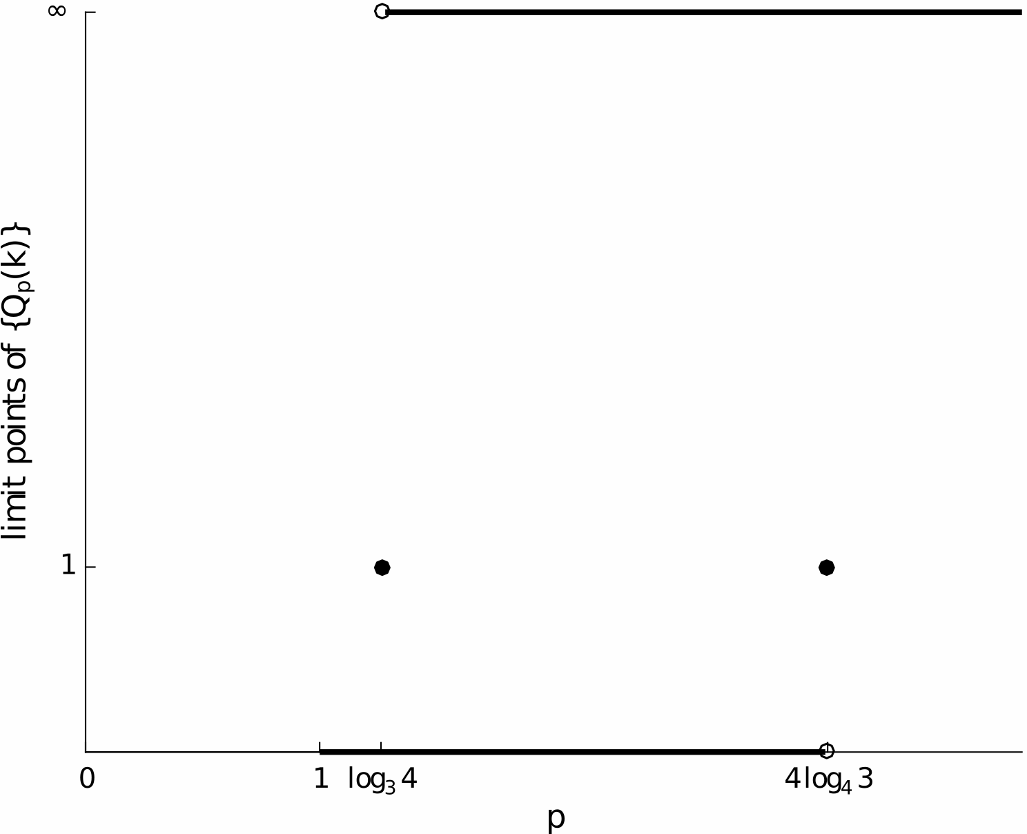
Refer to caption — Figure 1: $Q$ convergence-order profile for $\{x_{k}\}$ defined in Example 2.7. This is a graph of the limit points of $Q_{p}(k)$ as a function of $p$ . The vertical scale is not to scale.

This sequence does not have a $Q$ -order, as $q_{l}=\operatorname{log}_{3}4\approx 1.26<q_{u}=4\operatorname{log}_{4}3% \approx 3.17$ , but it converges with (exact) $R$ -order $2$ , as defined later. We note the classical statement in this case, ” $\{x_{k}\}$ converges with $Q$ -order (at least) $\operatorname{log}_{3}4\approx 1.26$ and with $R$ -order (at least) $2$ ”, which no longer holds in the setting of this paper.

An elementary example shows that in case of convergence with $Q$ -order $p_{0},$ apart of finite nonzero values of one (or both) of the asymptotical constants $\underline{Q}_{p_{0}}\leq\bar{Q}_{p_{0}}$ , any of the following relations may hold:

$\displaystyle\underline{Q}_{p_{0}}$	$\displaystyle=\bar{Q}_{p_{0}}=+\infty,$	(15)
$\displaystyle\underline{Q}_{p_{0}}$	$\displaystyle=\bar{Q}_{p_{0}}=0,$	(16)
$\displaystyle\underline{Q}_{p_{0}}$	$\displaystyle=0\textrm{ and}\ \bar{Q}_{p_{0}}=+\infty.$	(17)

Example 2.8

Let

x_{k}=2^{-2^{k}/k},\ \;\;\;y_{k}=2^{-k2^{k}},\;\;\;z_{k}=\begin{cases}x_{k},&k% \ \text{odd,}\\ y_{k},&k\text{ even.}\end{cases}

It is easy to verify that for $p_{0}=2,$ the sequences $\left\{x_{k}\right\},\left\{y_{k}\right\},\left\{z_{k}\right\}$ verify respectively (15), (16) and (17) ( $\{x_{k}\}$ was also considered in 60).

Schwetlick (20, Ü.4.2.3, p. 93) also considered an example of the type $x_{k}=e_{k}|\ln e_{k}|$ , $y_{k}=e_{k}/|\ln e_{k}|$ , for the errors $e_{k}$ converging with exact $Q$ -order $2$ .

Potra 16 considered

e_{k}=\begin{cases}e_{k+1}=2e_{k}e_{k-1}^{2},&k\ \text{even,}\\ e_{k+1}=e_{k}e_{k-1}^{2},&k\text{ odd,}\end{cases}

which has $Q$ -order $2$ and $\bar{Q}_{2}=+\infty$ .

Jay 35 considered the sequence of the type $x_{k}=k2^{-2^{k}}$ , $k$ even, $x_{k}=2^{-2^{k}}/k$ , $k$ odd, which satisfies (17) for $p_{0}=2$ .

One may easily find examples when $\underline{Q}_{p_{0}}=0$ and $\bar{Q}_{p_{0}}$ is finite, nonzero, or, on the other hand, when $\underline{Q}_{p_{0}}$ is finite, nonzero and $\bar{Q}_{p_{0}}=+\infty$ . Jay 35 considered the sequence $x_{k}=x_{k-1}^{q}/k$ , $k$ odd, $x_{k}=x_{k-1}^{q}$ , $k$ even, for $q\geq 1$ , $x_{0}=1$ , for which one obtains $\underline{Q}_{q}=0$ and $\bar{Q}_{q}=1$ .

Further examples, to be analyzed either elementary or with the aid of the results from this paper, were given by Potra and Pták (19, p. 93): $x_{k+1}=(x_{k})^{p-\frac{1}{k}}$ , $k\geq 1$ , $x_{1}=\theta$ , $0<\theta<1$ and also $x_{2k}=\theta^{(rs)^{k}}$ , $x_{2k+1}=\theta^{r^{k}s^{k+1}}$ , $0<\theta<1<r<s$ .

Remark 2.9

Despite the fact that conditions (15)–(17) may seem rather abstract (or, at least, suitable for scholar examples), they do occur in relevant situations from theory or practice. For a nontrivial illustration, we refer the reader to a computational optimization problem (56, p. 252 and Ch. 7), where one has $p_{0}=2$ and $\underline{Q}_{2}=\bar{Q}_{2}=+\infty$ .

Remark 2.10

When $\bar{Q}_{1}=0,$ i.e.,

\lim_{k\rightarrow\infty}\frac{e_{k+1}}{e_{k}}=0,

it is said that the sequence converges (at least) $Q$ -superlinearly. The convergence is strict $Q$ -superlinearly, when $q_{l}=1$ (i.e., $\bar{Q}_{p}=+\infty$ , $\forall p>1$ ); there are three cases in this situation: $q_{l}=q_{u}=1$ , i.e., $Q$ -order $1$ (see Example 3.6), $1=q_{l}<q_{u}<+\infty$ , resp. $1=q_{l}$ , $q_{u}=+\infty$ (see Example 2.14 b), formula (24)).

It is worth noting that one may also obtain $q_{l}=1$ , $q_{u}=+\infty$ in lack of $Q$ -superlinear (and even linear) convergence, shown in Example 2.14 d), formula (25)), as $\bar{Q}_{1}=+\infty$ .

Remark 2.11

Returning to the comments from Remark 2.6, we note that the comparison of the convergence of two sequences $\{x_{k}\}$ , $\{y_{k}\}$ having errors $\{e_{k}^{\prime}\}$ resp. $\{e_{k}^{\prime\prime}\}$ is important in particular in the field of the acceleration of the convergence of sequences, when sequences with (at most) linear convergence are considered; here it is said that $\{x_{k}\}$ converges faster than $\{y_{k}\}$ if (see, e.g., 6):

\lim_{k\rightarrow\infty}\frac{e_{k}^{\prime}}{e_{k}^{\prime\prime}}=0\quad(% \textrm{also denoted by\ }e_{k}^{\prime}=o(e_{k}^{\prime\prime}),\textrm{\ as % \ }k\rightarrow\infty).

(18)

Now we see that this definition makes sense not only if the $Q$ -orders of the two sequences are different, but even if they are equal, as the above condition is norm-independent.

To show this, we consider the terminology proposed by Jay 35 for a sequence converging with $Q$ -order $p_{0}>1$ , who defined that the convergence is with:

•

$Q$ -suborder $p_{0}$ if $\bar{Q}_{p_{0}}=\infty$ ,
•

$Q$ -superorder $p_{0}$ if $\bar{Q}_{p_{0}}=0$ .

The last terminology is in fact widely used - recall the superquadratic convergence (for $\bar{Q}_{2}=0$ ), supercubic, etc.).

Now we see that for sequences with $Q$ -order $p_{0}>1$ we can briefly say that:

•

$Q$ -superconvergence is faster than exact $Q$ -convergence (in the sense of (4) or (6));
•

exact $Q$ -convergence is faster than $Q$ -subconvergence;
•

(consequently) $Q$ -superconvergence is faster than $Q$ -subconvergence.

This can be illustrated by the following sequences having $Q$ -order $2$ : $\{2^{-k2^{k}}\}$ ( $Q$ -superquadratic), $\{2^{-2^{k}}\}$ (exact $Q$ -order $2$ ), $\{2^{-2^{k}/k}\}$ ( $Q$ -subquadratic).

2.1.2 Computational convergence orders, based on the corrections xk+1-xk and the nonlinear residuals F(xk)

We consider now some quantities which do not require the limit $x^{\ast}$ , for which we adopt the terminology computational convergence orders. As some of them require the knowledge of the order $p_{0}$ itself, we keep in mind that perhaps a more proper terminology for those would be semi-computational.

As a notation, for the corresponding convergence orders based on corrections we shall add a prime mark (e.g., $C^{\prime}$ ) as in 60, while for those based on nonlinear residuals, two prime marks (e.g., $C^{\prime\prime}$ ).

Corrections.

We introduce another notation, for the corrections (including their norms too):

s_{k}=\|x_{k+1}-x_{k}\|.

In 1974 Dennis and Moré 28 obtained a result which shows that if a sequence converges $Q$ -superlinearly, then the errors and corrections converge precisely at the same rate (Lemma 3.14 from subsubsection 3.2.1).

In 1984, Potra and Pták 19 shown that a sequence converges $Q$ -superlinearly iff the corrections converge $Q$ -superlinearly (Proposition 3.13); in 1997 Walker 21 gave a different proof, also presented later.

In 1982, Beyer and Stein 61 considered, for sequences in $\mathbb{R}$ , the quantity

\frac{\operatorname{log}\frac{s_{k}}{s_{k+1}}}{\operatorname{log}\frac{s_{k-1}% }{s_{k}}},

(19)

equivalent to $Q_{\Lambda}^{\prime}$ defined below.

Three years later, Brezinski 9 proposed the use of the corrections $x_{k+1}-x_{k}$ instead of the (unknown) errors $x^{\ast}-x_{k}$ in the definitions of the convergence orders studied there ( $Q_{L},Q_{\Lambda}$ and exact $Q$ -order).

In 1990, Beyer, Ebanks and Qualls 60, taking the same approach, considered

Q_{p_{0}}^{\prime}\left(k\right):=\frac{s_{k+1}}{s_{k}^{p_{0}}}

with the resulted definitions being denoted correspondingly by $C^{\prime},Q^{\prime},Q_{L}^{\prime}$ and $Q_{\Lambda}^{\prime}$ ; we use here the same convention for denoting $Q_{\varepsilon}^{\prime},Q_{I,\varepsilon}^{\prime}$ . These authors proved the following fundamental results: for $p_{0}>1$ , the errors and corrections converge simultaneously to zero with the same convergence order, and therefore each convergence order is equivalent to its corresponding computational one. The following extended relation resulted:

\left\{C_{p_{0}},C_{p_{0}}^{\prime}\right\}\Rightarrow\left\{Q,Q_{L},Q_{% \Lambda},Q^{\prime},Q_{L}^{\prime},Q_{\Lambda}^{\prime}\right\}.

However, the considered assumptions were very strong when proving $\left\{C_{p_{0}},C_{p_{0}}^{\prime}\right\}$ and ” $Q^{\prime}\Rightarrow Q$ ”: $\{x_{k}\}$ was assumed as a monotone sequence from $\mathbb{R}$ (see (60, Sect. 4)). We shall see that for the general setting, some results from 19 and 28 may be used instead to obtain simplified proofs.

In 2010, Grau-Sánchez, Noguera and Gutiérrez 38, while studying connections between $Q_{\Lambda}$ - and $Q_{\Lambda}^{\prime}$ -orders (in the case of a sequence from $\mathbb{R}$ with $C$ -order $p$ ) considered the ”extrapolated convergence order”

\frac{\ln\frac{|x_{k+1}-\tilde{\alpha}_{k+1}|}{|x_{k}-\tilde{\alpha}_{k}|}}{% \ln\frac{|x_{k}-\tilde{\alpha}_{k}|}{|x_{k-1}-\tilde{\alpha}_{k-1}|}},

(20)

where $\tilde{\alpha}_{k}=x_{k}-\frac{\left(\Delta x_{k-1}\right)^{2}}{\Delta^{2}x_{k% -2}},$ $k\geq 2,$ $\Delta x_{k}=x_{k+1}-x_{k}$ . This convergence order was obtained from $Q_{\Lambda}$ by replacing the unknown limit with an extrapolation $\tilde{\alpha}_{k}$ given by the Aitken $\Delta^{2}$ method (in order to use only the terms known at the step $k$ ). However, this convergence order is valid only in the one dimensional case, since the Aitken $\Delta^{2}$ acceleration process does not have a direct extension to $\mathbb{R}^{n}$ .

We do not pursue this definition as, for high convergence orders, it is equivalent to $Q_{\Lambda}^{\prime}$ .

In 2012, Grau-Sánchez, Noguera, Grau and Herrero 37 considered another extrapolated convergence order

\tfrac{\ln\left|x_{k}-\tilde{\alpha}_{k}\right|}{\ln\left|x_{k-1}-\tilde{% \alpha}_{k-1}\right|},

(21)

for a sequence from $\mathbb{R}$ , having $C$ -order $p$ . Assuming $C$ -order, they shown some connections to the convergence orders (22) and (23) below.

In 38 and 37 the authors used the technique of asymptotic expansions in order to relate different convergence orders of $\{e_{k}\}$ , $\{s_{k}\}$ and $\{f(x_{k})\}$ for sequences $\{x_{k}\}$ from $\mathbb{R}$ . However, this approach could not be extended to the case of several dimensions.

Remark 2.12

It is important to keep in mind that the $C^{\prime}$ -, $Q^{\prime}_{\varepsilon}$ -, $Q^{\prime}_{I,\varepsilon}$ -orders are semi-computational orders, as they require the (supposed) unknown order, while the logarithm-based $Q^{\prime}_{L}$ - and $Q^{\prime}_{\Lambda}$ -orders are (fully) computational orders, i.e., they require neither the limit $x^{\ast}$ nor the order $p$ in their expressions.

As certain numerical experiments (see 39 and the references therein) have not revealed a clear superiority of $Q^{\prime}_{\Lambda}$ over $Q^{\prime}_{L}$ , the later seems to be the most convenient to use in practice (and in theory too: see (56, p. 252 and Ch. 7), (63, p. 210, p. 226), 18 and 17). Moreover, Propositin 3.3 and Theorem 3.15 will show, in terms we will define later, that $q_{l}=q^{\prime}_{l}=\underline{Q}_{L}$ and $q_{u}=q^{\prime}_{u}=\bar{Q}_{L}$ .

Nonlinear residuals.

Other computational convergence orders were considered in the context of solving nonlinear systems of equations $F(x)=0$ , $F:\mathbb{R}^{n}\rightarrow\mathbb{R}^{n}$ , with solution $x^{\ast}$ . For simplicity, we shall denote $F_{k}:=F(x_{k})$ (resp. $f_{k}$ when $n=1$ ).

In 1981, Păvăloiu 25 defined the exact convergence order $p_{0}>1$ corresponding to (4) by

A\|F_{k}\|^{p_{0}}\leq\|F_{k+1}\|\leq B\|F_{k}\|^{p_{0}},\ \;\;\forall k\geq 0,

while in 1995, he introduced in 22 the expression

\frac{\ln|f_{k+1}|}{\ln|f_{k}|}

(22)

and shown its equivalence to $Q^{\prime}_{L}$ . Also, while extending his results from 1999 24, he introduced in an unpublished manuscript 23 (posted on his website) the measure

\frac{\ln|f_{k+1}/f_{k}|}{\ln|f_{k}/f_{k-1}|}

(23)

in connection with the above ones. However, since the manuscript was not published as of 2011, the credit of first publishing this measure goes to Petković, who mentioned in passing the above expression in a note published in SIAM J. Numer. Anal. (2011).

Several computational aspects regarding these quantities were subsequently analyzed (see, e.g., 39 and the references therein).

2.2 R-convergence orders.

The root convergence order ( $R$ -order) requires weaker conditions than the $C$ - and $Q$ -orders, but unfortunately at the price of loosing its theoretical importance and its practical applications. As we have quoted in the Introduction, “The distinction between $Q$ - and $R$ -convergence is […] essentially sacred to workers in the area of computational optimization” (49, p. 49), meaning that the $R$ -order is a much less powerful notion.

In Example 3.11 is presented a sequence for which, depending on the parameters, the lower $Q$ -order $q_{l}$ is arbitrary close to $1$ from above, while the (exact) $R$ -order is arbitrary high (and even higher is the upper $Q$ -order $q_{u}$ ).

We shall review certain results, but not treat all of them in the same detail as we will for the $C$ - and $Q$ -orders.

In 1970, Ortega and Rheinboldt (32, 9.2) introduced and studied the root convergence factors, which we denote here by $\bar{R}_{p}\left\{x_{k}\right\}$ :

\bar{R}_{p}\left\{x_{k}\right\}=\left\{\begin{array}[c]{c}\limsup\limits_{k% \rightarrow\infty}\,(e_{k})^{\frac{1}{k}},\text{ if}\;p=1,\\ \limsup\limits_{k\rightarrow\infty}\,(e_{k})^{\frac{1}{p^{k}}},\text{ if}\;p>1% .\end{array}\right.

Unlike the quotient factors, the root factors do not relate each two consecutive terms, but consider some averaged asymptotic quantities.

They proved a Proposition similar to Proposition 2.5, but here $1$ takes the role of $+\infty$ for $\bar{Q}_{p}$ .

Proposition 2.13

(32, 9.2.3) Exactly one of the following conditions holds:

a) $\bar{R}_{p}=0,\ \forall p\in[1,+\infty);$

b) $\bar{R}_{p}=1,\ \forall p\in[1,+\infty);$

c) $\exists p_{0}\in[1,+\infty)$ s.t. $\bar{R}_{p}=0,$ $\forall p\in[1,p_{0})$ and $\bar{R}_{p}=1,$ $\forall p\in\left(p_{0},+\infty\right).$

The lower $R$ -order, which we denote here by $r_{l}$ (instead of $O_{R}\left\{x_{k}\right\}$ in (32, 9.2)), defined by

r_{l}=\left\{\begin{array}[c]{c}\infty,\text{\ \ \ if \ }\bar{R}_{p}=0,\ % \forall p\geq 1,\\ \inf\big{\{}p\in[1,\infty):\bar{R}_{p}=1\big{\}},\end{array}\right.

stood in 32 and in many subsequent works as the definition of the root convergence order.

Remark 2.14

a) (32, p. 290) If there exists a $p_{0}$ with $\bar{R}_{p_{0}}<1,$ then for any $\varepsilon>0$ with $\bar{R}_{p_{0}}+\varepsilon<1,$ there exists a $k_{0}\geq 0$ such that either

e_{k}\leq\left(\bar{R}_{p_{0}}+\varepsilon\right)^{k},\;\;\;\forall k\geq k_{0% },\text{ if}\;p_{0}=1,

e_{k}\leq\left(\bar{R}_{p_{0}}+\varepsilon\right)^{p_{0}^{k}},\;\;\;\forall k% \geq k_{0},\text{ if}\;p_{0}>1.

b) The value $r_{l}$ arises in the analysis of the speed of convergence of sequences with the errors satisfying different recurrence inequalities.

The simplest ones appear in usual circumstances for the secant method (see 4, 41, and also 51):

e_{k+1}\leq Ae_{k}\cdot e_{k-1}

and they yield the well-known $r_{l}$ -order $(1+\sqrt{5})/2\approx 1.6$ . It is important to note that the secant method then attains the same value also for the lower $Q$ -order $q_{l}$ (see 4, 41).

For the more general inequalities

e_{k+1}\leq A\textstyle\prod\limits_{i=0}^{m}(e_{k-i})^{\alpha_{i}},\quad k% \geq m,\ c_{k},\alpha_{k}\geq 0,

Schmidt 33, Burmeister and Schmidt 58, 59 resp. Potra and Pták (19, p. 107) determined in a series of works the lower $R$ -order $r_{l}$ .

It is interesting to note that for such inequalities, Herzberger and Metzner 27 and then Potra 16 gave certain sufficient conditions for the lower bound $q_{l}$ . Potra 16 has also noted that the above inequalities do not necessarily attract lower order $q_{l}$ greater than one: take

e_{k+1}=\begin{cases}(e_{k})^{k},&k>1\ \text{\rm is a power of }2,\\ e_{k}e_{k-1},&{\rm otherwise},\end{cases}

(24)

with $e_{0}=e_{1}=\frac{1}{2}$ . This sequence satisfies $e_{k+1}\leq e_{k}e_{k-1}$ (which immediately attracts $\bar{Q}_{1}=0$ and $r_{l}\geq(1+\sqrt{5})/2$ ), but in fact $\bar{Q}_{p}=+\infty$ , $\forall p>1$ (and $q_{u}=\bar{Q}_{L}=+\infty$ , as we shall see).

Certain iterative methods have lead to some different inequalities, of the type (32, Th. 9.2.9.)

e_{k+1}\leq e_{k}\sum_{j=0}^{m}\gamma_{j}e_{k-j},\;\;\forall k\geq m,\textrm{ % with }\gamma_{1},...,\gamma_{m}\geq 0,

or of other types, analyzed in 30 (see also 50).

c) As noted in (32, N.R. 9.2.1), the $\bar{R}_{1}$ factor has been used implicitly in much work concerning iterative processes for linear systems of equations, see, e.g., Varga 47. For nonlinear systems, it was used explicitly by Ortega and Rockoff 31.

d) Some connections between the errors and their majorizing sequences were made by Dennis Jr. in 29 (see also (49, p. 49)). Potra 16 has noticed that the lower $R$ -order $r_{l}$ is consistent with the natural ordering of sequences, while the lower $Q$ -order $q_{l}$ is not: given $\{x_{k}\},\{y_{k}\}$ with errors $\{e_{k}^{\prime}\}$ , resp. $\{e_{k}^{\prime\prime}\}$ , if $e_{k}^{\prime}\leq e_{k}^{\prime\prime}$ and $\{y_{k}\}$ has $r_{l}$ order $p_{0}$ then so has $\{x_{k}\}$ ; however, this statement does not hold for the lower $Q$ -order $q_{l}$ , as one may take $\{x_{k}\}$ from Example 2.7 and $y_{k}=2^{-2^{k}}$ . A more disturbing example was given by Jay 35, for $y_{k}=2^{-2^{k}}$ and

x_{k}=\begin{cases}2^{-2^{k}},&k\ {\rm even},\\ 2^{-3^{k}},&k\ {\rm odd}.\end{cases}

(25)

At the first sight, since $e_{k}^{\prime}\leq e_{k}^{\prime\prime}$ , the speed of $\{x_{k}\}$ seems higher than of the (exact) $Q$ -quadratic $\{y_{k}\}$ , but though, $\{x_{k}\}$ does not attain even $Q$ -linear convergence, as $\bar{Q}_{1}=\infty$ (we shall see that in this case the upper $Q$ -order is $q_{u}=\bar{Q}_{\Lambda}=\infty$ ). Another example was given in (24) above.

In 1973, Brent, Winograd and Wolfe 51 considered the following expressions, which we denote here by

	$\displaystyle\underline{R}_{L}:=$	$\displaystyle\liminf\limits_{k\rightarrow\infty}\big{\|}\ln e_{k}\big{\|}^{\frac% {1}{k}},$		(26)
	$\displaystyle\bar{R}_{L}:=$	$\displaystyle\limsup\limits_{k\rightarrow\infty}\big{\|}\ln e_{k}\big{\|}^{\frac% {1}{k}}$

(in 52 Brent considered in the same year only $\underline{R}_{L}$ ). The sequence was said that converges with $R_{L}$ -order $p_{0}>1$ if $\underline{R}_{L}=\bar{R}_{L}=p_{0}$ , i.e., in a single condition,

\lim_{k\rightarrow\infty}\big{|}\ln e_{k}\big{|}^{\frac{1}{k}}=p_{0}.

(27)

They noted that the $C$ -order $p_{0}>1$ easily implies $R_{L}$ -order $p_{0}$ .

In 1979, Schwetlick 20 considered the upper $R$ -order

\underline{R}_{p}\left\{x_{k}\right\}=\begin{cases}\liminf\limits_{k% \rightarrow\infty}\,(e_{k})^{\frac{1}{k}},&\text{ if}\;p=1,\\ \liminf\limits_{k\rightarrow\infty}\,(e_{k})^{\frac{1}{p^{k}}},&\text{ if}\;p>% 1,\end{cases}

and (in the notations of this paper)

r_{u}=\begin{cases}\infty,\text{\ \ \ if \ }\underline{R}_{p}=0,\ \forall p% \geq 1,\\[5.69054pt] \sup\big{\{}p\in[1,\infty):\underline{R}_{p}=0\big{\}},\end{cases}

he defined the convergence with $R$ -order $p_{0}$ if $p_{0}=r_{l}=r_{u}.$

Similarly to the case of the $Q$ -order, the sequence is said that converges $R$ -superlinearly if

\lim_{k\rightarrow\infty}(e_{k})^{\frac{1}{k}}=\bar{R}_{1}=0.

Remark 2.15

Analogously to Remark 2.14, whenever exists a $p_{0}$ with $\underline{R}_{p_{0}}>0,$ then for any $\varepsilon>0$ with $0<\underline{R}_{p_{0}}-\varepsilon,$ there is a $k_{0}\geq 0$ such that either

\left(\underline{R}_{p_{0}}-\varepsilon\right)^{k}\leq e_{k},\quad\forall k% \geq k_{0},\text{ if}\;p_{0}=1,

\left(\underline{R}_{p_{0}}-\varepsilon\right)^{p_{0}^{k}}\leq e_{k},\quad% \forall k\geq k_{0},\text{ if}\;p_{0}>1.

In 1989, Potra 16 has introduced and studied some further measures for the $R$ -convergence order, which we denote here by $R_{\varepsilon}$ , resp. $R_{I,\varepsilon}$ :

•

$\{x_{k}\}$ converges with $R_{\varepsilon}$ -order $p_{0}>1$ if

$\displaystyle\lim_{k\rightarrow\infty}(e_{k})^{\frac{1}{(p_{0}-\varepsilon)^{k% }}}$ $\displaystyle=0,\quad\forall\varepsilon>0,$

$\displaystyle\lim_{k\rightarrow\infty}(e_{k})^{\frac{1}{(p_{0}+\varepsilon)^{k% }}}$ $\displaystyle=1,\quad\forall\varepsilon>0;$
•

$\{x_{k}\}$ converges with $R_{I,\varepsilon}$ -order $p_{0}>1$ if $\forall\varepsilon>0,$ $\exists a,b>0$ and $0<\eta,\theta<1$ such that

$a\,\eta^{\left(p_{0}+\varepsilon\right)^{k}}\leq e_{k}\leq b\,\theta^{\left(p_% {0}-\varepsilon\right)^{k}},\;\;\forall k\geq 0.$

The exact $R$ -order of convergence was also defined here – analogously to the definition of the exact $Q$ -order (4) – as being $p_{0}>1$ if $\exists A,B>0$ , $0<\eta,\theta<1$ such that

A\cdot\eta^{(p_{0})^{k}}\leq e_{k}\leq B\cdot\theta^{(p_{0})^{k}},\;\;\forall k% \geq 0;

(28)

we see that this definition can be immediately connected to the following one, analogous to (6):

0<\underline{R}_{p_{0}}<\bar{R}_{p_{0}}<\infty.

(29)

Potra has also considered the lower and upper $R$ -orders, when noting that if a sequence has exact $R$ -order $p_{0}$ then $r_{l}=r_{u}=p_{0}$ .

Comparing the list of $Q$ - and $R$ -orders, the definition of $R_{\Lambda}$ was not given before, so we consider it here, by denoting the expressions

\underline{R}_{\Lambda}:=\liminf\limits_{k\rightarrow\infty}\big{|}\ln\tfrac{e% _{k+1}}{e_{k}}\big{|}^{\frac{1}{k}},\quad\bar{R}_{\Lambda}:=\limsup\limits_{k% \rightarrow\infty}\big{|}\ln\tfrac{e_{k+1}}{e_{k}}\big{|}^{\frac{1}{k}}

and by defining the $R_{\Lambda}$ -order $p_{0}\geq 1$ when $\underline{R}_{\Lambda}=\bar{R}_{\Lambda}=p_{0}$ , i.e., when

\lim_{k\rightarrow\infty}\big{|}\ln\tfrac{e_{k+1}}{e_{k}}\big{|}^{\frac{1}{k}}% =p_{0}.

(30)

3 Results relating the high (computational) convergence orders

In this section we consider $p>1$ and present the relationships of different definitions of the (computational) convergence orders, with full proofs in the case of the $C$ - and $Q$ -orders.

3.1 Relationships between the convergence orders

The equivalences and implications mentioned in the previous section can be summarized as:

	$\displaystyle\left\{Q_{\varepsilon},Q_{I,\varepsilon},Q_{L}\right\}$	$\displaystyle\Rightarrow\left\{R_{\varepsilon},R_{I,\varepsilon},R_{L}\right\}% ,\;\;\;\text{ \cite[cite]{\@@bibref{Authors Phrase1YearPhrase2}{Potra89}{\@@citephrase{(}}{% \@@citephrase{)}}},}$
	$\displaystyle C_{p_{0}}$	$\displaystyle\Rightarrow\left\{Q,Q_{L},Q_{\Lambda}\right\},\;\;\;\;\text{ % \cite[cite]{\@@bibref{Authors Phrase1YearPhrase2}{BEQ90}{\@@citephrase{(}}{% \@@citephrase{)}}}.}$

At this point we can simply merge the equivalences from the two statements above and write the conclusion.

However, as we intend to provide a self-contained material, we include the proofs of the equivalence of the $Q$ -orders, some of them much simplified.

3.1.1 C- and Q-convergence orders

We shall need the three auxiliary results below.

Lemma 3.1

(60, lemma 2.1)

(i): If $\bar{Q}_{p}<\infty,$ then $Q_{s}\left(k\right)\rightarrow 0$ for all $s<p$ , and so $p\leq q_{l};$
(ii): if $\underline{Q}_{p}>0,$ then $Q_{s}\left(k\right)\rightarrow\infty$ for all $p<s$ and so $q_{u}\leq p;$
(iii): if $p<q_{l},$ then $Q_{p}\left(k\right)\rightarrow 0;$
(iv): if $q_{u}<p,$ then $Q_{p}\left(k\right)\rightarrow\infty$ .

Relations (iii) and (iv) show that $q_{l}\leq q_{u}$ and justify the terminology ”lower” and ”upper”.

Proof. 60 For (i), if $\bar{Q}_{p}<\infty$ and $s<p,$ then

Q_{s}(k)=\frac{e_{k+1}}{e_{k}^{s}}=e_{k}^{p-s}Q_{p}(k)\rightarrow 0,\quad\text% {as }k\rightarrow\infty.

For (iii), suppose $p<q_{l}$ and choose $s\in\left(p,q_{l}\right).$ By definition of $q_{l},$ then, $\bar{Q}_{s}<\infty$ . Now, by (i), $Q_{p}\left(k\right)\rightarrow 0.$

The other statements are proved in a similar manner.

Remark 3.2

Ortega and Rheinboldt have previously obtained (i) and (ii) in (32, 9.1), see Proposition 2.5.

Potra obtained the following general result, interesting in its own, which will help us relating some quantities to their corresponding computational versions.

Proposition 3.3

(16, Prop. 1.1) The following relations hold:

\underline{Q}_{L}:=\liminf_{k\rightarrow\infty}\frac{\ln e_{k+1}}{\ln e_{k}}=q% _{l}

(31)

and

\bar{Q}_{L}:=\limsup_{k\rightarrow\infty}\frac{\ln e_{k+1}}{\ln e_{k}}=q_{u}.

Proof. 16 Let

1<\underline{Q}_{L}=p_{0}.

Then for any $\varepsilon>0$ with $p_{0}-\varepsilon>1$ , there exists $k_{0}$ such that

\tfrac{\ln e_{k+1}}{\ln e_{k}}>p_{0}-\varepsilon,\quad k\geq k_{0}.

We may assume that $\ln e_{k}<0$ , and we obtain

\ln e_{k+1}<(p_{0}-\varepsilon)\ln e_{k},\quad k\geq k_{0},

so that

e_{k+1}<e_{k}^{p_{0}-\varepsilon},\quad k\geq k_{0}.

This proves that $\bar{Q}_{p_{0}-\varepsilon}\leq 1<\infty$ and, by Lemma 3.1 (i), we get

p_{0}\leq q_{l}.

Suppose that

p_{0}<s<q_{l}.

It follows by Lemma 3.1 (iii) that $Q_{s}\left(k\right)\rightarrow 0,$ so there is $c>0$ such that $Q_{s}\left(k\right)\leq c,$ $\forall k\geq 0,$ i.e.,

e_{k+1}\leq ce_{k}^{s},\quad k\geq 0.

But then

\ln e_{k+1}\leq\ln c+s\ln e_{k},

which leads to

\liminf_{k\rightarrow\infty}\tfrac{\ln e_{k+1}}{\ln e_{k}}\geq s+\lim_{k% \rightarrow\infty}\tfrac{\ln c}{\ln e_{k}}=s>p_{0},

which is a contradiction. Hence, we have proved that $\underline{Q}_{L}=q_{l}.$

Analogously, $\bar{Q}_{L}=p_{1}$ implies $p_{1}=q_{u}.$

Lemma 3.4

(60, lemma 3.3) If

\lim\inf Q_{\Lambda}\left(k\right)>0,

then $\{e_{k}\}$ is monotone decreasing starting from a step $k\geq k_{0}$ .

Proof. 60 For some some $\varepsilon>0$ sufficiently small, $\exists k_{0}\geq 0$ such that $Q_{\Lambda}(k)>\varepsilon,$ $\forall k\geq k_{0}.$ Hence, the numbers $\ln\tfrac{e_{k+1}}{e_{k}}$ all have the same sign $\forall k\geq k_{0}$ . If they were positive, then we would have $e_{k+1}>e_{k}$ , contradictory to the convergence of $\{x_{k}\}.$ Therefore, they are all negative and $e_{k+1}<e_{k}.$

We present now the result relating the $C$ - and $Q$ -orders, and we choose to incorporate Proposition 3.3.

Theorem 3.5

(cf. 16, 60) Consider a given norm $\|\cdot\|$ in $\mathbb{R}^{n}$ and a convergent sequence $\{x_{k}\}$ to some $x^{\ast}\in\mathbb{R}^{n}$ . Then, given some $p_{0}>1$ , in the above notations we have:

C_{p_{0}}\underset{\nLeftarrow}{\Rightarrow}\left\{Q,Q_{\varepsilon},Q_{I,% \varepsilon},Q_{L},Q_{\Lambda}\right\}.

(32)

Moreover,

\underline{Q}_{L}=q_{l}\quad\textrm{and }\bar{Q}_{L}=q_{u}.

(33)

Proof. We give the proof in five steps: A. $C_{p_{0}}\underset{\nLeftarrow}{\Rightarrow}Q_{L}$ , B. $Q\Leftrightarrow Q_{\varepsilon}$ , C. $Q_{\varepsilon}\Leftrightarrow Q_{I,\varepsilon}$ , D. $Q\Leftrightarrow Q_{L}$ and E. $Q_{\Lambda}\Leftrightarrow Q_{L}$

A1 ( $C_{p_{0}}\Rightarrow Q_{L}$ ). The simplest approach is (also mentioned in 51) to take logarithms in (2). The proof in 60 used an approach similar to Lemma 3.1.

A2 ( $Q_{L}\nRightarrow C_{p_{0}}$ ) 60 Consider any of the sequences from Example 2.8.

B. The relation is obvious.

C1 ( $Q_{\varepsilon}\Rightarrow Q_{I,\varepsilon}$ ) Let $\varepsilon>0$ such that $p_{0}-\varepsilon>1.$ Since $Q_{p-\varepsilon}\rightarrow 0$ , it follows that exists $b$ such that $Q_{p_{0}-\varepsilon}\leq b,$ $\forall k\geq 0,$ i.e., the second inequality in the definition of $Q_{I,\varepsilon}.$ The first inequality is obtained in the same way.

C2 ( $Q_{I,\varepsilon}\Rightarrow Q_{\varepsilon}$ ) Suppose for some $p_{0}>1$ and $\varepsilon>0$ with $p_{0}-\varepsilon>1$ we have

a(e_{k})^{p_{0}+\varepsilon}\leq e_{k+1}\leq b(e_{k})^{p_{0}-\varepsilon},% \quad\forall k\geq 0.

The second inequality implies $\bar{Q}_{p_{0}-\varepsilon}\leq b<\infty,$ and by Lemma 3.1 (i), $\lim Q_{q}\left(k\right)=0,\ \ \forall q$ s.t. $1<q<p_{0}-\varepsilon.$

The first inequality (valid for all $\varepsilon>0$ ) implies $\underline{Q}_{p_{0}+\varepsilon}\geq a>0$ and again by Lemma 3.1 (ii), $\lim Q_{s}\left(k\right)=+\infty,\ \ \forall s$ with $p+\varepsilon<s.$

The assertion follows since $\varepsilon$ can be taken arbitrarily small.

D. (16, Prop. 1.1) Using the above result, we get $Q_{L}\Rightarrow\bar{Q}_{L}=\underline{Q}_{L}=p_{0}\Rightarrow q_{l}=q_{u}=p_{% 0}\Rightarrow Q$ and vice versa.

E1 ( $Q_{\Lambda}\Rightarrow Q_{L}$ ) 60 We notice that, by B and D, we have that $Q_{L}\Leftrightarrow Q_{\varepsilon}$ , so it suffices to show that $Q_{\Lambda}\Rightarrow Q_{\varepsilon}$ .

Let $Q_{\Lambda}(k)\rightarrow p_{0}>1.$ For any $\varepsilon>0,$ we have $Q_{\Lambda}(k)<p_{0}+\varepsilon$ for all $k$ sufficiently large, and using Lemma 3.4 we get

\ln\tfrac{e_{k+2}}{e_{k+1}}>(p_{0}+\varepsilon)\ln\tfrac{e_{k+1}}{e_{k}},

which gives

\tfrac{e_{k+2}}{(e_{k+1})^{p_{0}+\varepsilon}}>\tfrac{e_{k+1}}{(e_{k})^{p_{0}+% \varepsilon}},

i.e., $Q_{p_{0}+\varepsilon}\left(k+1\right)>Q_{p_{0}+\varepsilon}\left(k\right),$ $\forall k\geq k_{0}.$

Considering now $\frac{\varepsilon}{2}$ instead of $\varepsilon,$ we obtain similarly that

Q_{p_{0}+\frac{\varepsilon}{2}}\left(k+1\right)>Q_{p_{0}+\frac{\varepsilon}{2}% }\left(k\right),\;\;\forall k\geq k_{1}.

(34)

We prove that the monotone sequence $\left\{Q_{p_{0}+\varepsilon}\left(k\right)\right\}$ is unbounded: $Q_{p_{0}+\varepsilon}\left(k\right)\rightarrow\infty.$ Otherwise, if $\exists M>0$ s.t. $\frac{e_{k+2}}{(e_{k+1})^{p_{0}+\varepsilon}}<M,$ for all $k,$ i.e., $\bar{Q}_{p_{0}+\varepsilon}<M,$ then according to Lemma 3.1 (i), this implies $\bar{Q}_{p_{0}+\frac{\varepsilon}{2}}=0$ in contradiction to the monotony from (34).

Similarly, one can prove that for any $\varepsilon>0$ with $p_{0}-\varepsilon>1,$ we have $Q_{\Lambda}\left(k\right)>p_{0}-\varepsilon$ for all $k$ sufficiently large and we get $Q_{p_{0}-\varepsilon}\left(k\right)\rightarrow 0.$

E2 ( $Q_{L}\Rightarrow Q_{\Lambda}$ ) 60 Assuming $Q_{L}(k)\rightarrow p_{0}>1,$ we have

\lim_{k\rightarrow\infty}Q_{\Lambda}(k)=\lim_{k\rightarrow\infty}Q_{L}\left(k% \right)\tfrac{Q_{L}\left(k+1\right)-1}{Q_{L}\left(k\right)-1}=p_{0}\tfrac{p_{0% }-1}{p_{0}-1}=p_{0}.

It is interesting to notice that $Q$ -convergence with order $p_{0}>1$ implies $\bar{Q}_{1}=0.$ However, the reverse is not true (i.e., $Q$ -superlinear convergence does not imply $Q$ -convergence with order $p_{0}>1$ ), as the following examples show.

Example 3.6

a) (32, E 10.1.4) (we follow here (19, p. 94)) Let $0<c<1/e$ and consider the sequence

x_{k+1}=-\tfrac{x_{k}}{\ln x_{k}},\;\;\;\;k\geq 0,x_{0}=c,

which converges superlinearly to $0 .$ Suppose there exists $p_{0}>1$ such that $\left\{x_{k}\right\}$ converges with $Q$ -order (and therefore with $Q_{I,\varepsilon}$ order) $p_{0}.$ Then $\forall\varepsilon>0$ with $p_{0}-\varepsilon>1,\exists b>0$ s.t. $x_{k+1}\leq bx_{k}^{p_{0}-\varepsilon}.$ Hence,

-\tfrac{x_{k}}{\ln x_{k}}\leq bx_{k}^{p_{0}-\varepsilon}\quad\textrm{or}\quad% \frac{\big{(}\frac{1}{x_{k}}\big{)}^{p_{0}-\varepsilon-1}}{\ln\frac{1}{x_{k}}}% \leq b,

for all $k$ sufficiently large, which contradicts the well known limit $\lim_{t\rightarrow\infty}\tfrac{t^{\alpha}}{\ln t}=\infty$ , for any $\alpha>0$ . As $Q_{L}(k)\rightarrow 1$ , we get $q_{l}=q_{u}=1$ .

b) Some simpler examples can be found either as explicitly given by $x_{k}=k^{-k}$ (52, p. 22), $x_{k}=10^{-k^{2}}$ 9, 60, $x_{k}=\frac{1}{k!}$ 35, or in the list of exercises, by $x_{k}=c^{-k^{2}}$ , $c>1$ (32, E.9.2.1.j). To show these assertions we can also use that $Q_{L}(k)$ or $Q_{\Lambda}(k)\rightarrow 1$ . Expression (24) of Potra gives yet another example.

Remark 3.7

We notice that the orders $Q_{\varepsilon},Q_{I,\varepsilon},Q_{L},Q_{\Lambda}$ do not have elements to define the strict $Q$ -superlinear convergence, when $\bar{Q}_{1}=0$ and $\bar{Q}_{p}=+\infty,$ $\forall p>1$ .

The $Q$ -superlinear convergence implies $R$ -superlinear convergence, as in any norm (32, 9.3.1)

\bar{R}_{1}\leq\bar{Q}_{1}.

In fact, $\bar{R}_{1}$ is a lower bound for $\bar{Q}_{1}$ in all norms from $\mathbb{R}^{n}$ .

It is interesting to see that sequences with infinite $Q$ -order exist too, as one can take $x_{k}=2^{-2^{2^{k}}}$ (from the list of exercises in (32, E.9.2.1)).

Remark 3.8

An important aspect we address now is the problem of changing the norms, as we have seen in Example 2.3 that for a given sequence in $\mathbb{R}^{n}$ the existence of the $C$ -order is norm-dependent. Ortega and Rheinboldt (32, 9.1.6) proved that the three relations $\bar{Q}_{p}=0$ , $\bar{Q}_{p}$ finite, $\bar{Q}_{p}=\infty$ are norm-independent. The same hold for $\underline{Q}_{p}$ , as one can easily verify (using also Lemma 3.1), which shows the norm-independence of the $Q$ -order. By the equivalence from Theorem 3.5, we conclude that the rest of the $Q$ -orders are norm independent too. This assertion will be further completed by the computational convergence orders, as we shall see in the following subsection.

It is important to recall that for sequences with $Q$ -order $p_{0}>1$ , while this $Q$ -order is norm-independent, the values of the quantities $\bar{Q}_{p_{0}}$ and $\underline{Q}_{p_{0}}$ however, if finite, are norm-dependent (32, E.9.1-1).

Remark 3.9

One can easily show that the sequence $\{x_{k}\}$ converges with $Q$ -order $p_{0}>1$ iff one of the the following sequences converges with the same order: $\{\frac{e_{k+1}}{e_{k}}\}$ , $\{e_{k+1}\cdot e_{k}\}$ or $\{(e_{k})^{\alpha}\}$ ( $\alpha>0$ arbitrary, given).

3.1.2 R-convergence orders

In 1972, Brent 52 stated, while in 1984, Potra and Pták 19 shown that

r_{l}=\underline{R}_{L}:=\liminf\limits_{k\rightarrow\infty}\big{|}\ln e_{k}% \big{|}^{\frac{1}{k}}.

(35)

In 1989 Potra 16 stated the equivalence $\{R_{\varepsilon},R_{I,\varepsilon},R_{L}\}$ , which can be easily proved.

In fact we may extend Theorem 3.5 and the above relations. For brevity, we choose to write $\{Q\}$ as a generic form for all the five equivalent $Q$ -type orders, $\{Q,Q_{\varepsilon},Q_{I,\varepsilon},Q_{L},Q_{\Lambda}\}$ . The same will be written in the sequel for $\{Q^{\prime}\}$ , $\{Q^{\prime\prime}\}$ , $\{R\}$ , $\{R^{\prime}\}$ and $\{R^{\prime\prime}\}$ .

Theorem 3.10

(cf. 16) In the assumptions of Theorem 3.5, we have:

C_{p_{0}}\underset{\nLeftarrow}{\Rightarrow}\{Q\}\underset{\nLeftarrow}{% \Rightarrow}\{R,R_{\varepsilon},R_{I,\varepsilon},R_{L},R_{\Lambda}\}

(36)

(with the equivalence of $R_{\Lambda}$ requiring the additional assumption $1<q_{l}\leq q_{u}<\infty$ ).

Moreover,

q_{l}=\underline{Q}_{L}\leq\underline{R}_{L}=\underline{R}_{\Lambda}=r_{l}\leq r% _{u}=\bar{R}_{L}=\bar{R}_{\Lambda}\leq\bar{Q}_{L}=q_{u}.

(37)

Proof. (cf. 16) We notice first that $Q_{I,\varepsilon}$ -order $p_{0}$ implies $R_{I,\varepsilon}$ -order $p_{0}$ (and therefore $\{Q\}\Rightarrow\{R_{\varepsilon},R_{I,\varepsilon},R_{L}\}$ , as mentioned above); this is obtained from the proofs of Propositions 9.3.2 and 9.3.3 in 32 and taking into account Proposition 2.13 above. A simpler approach results by considering directly (37), with $q_{l}=q_{u}$ .

The converse ” $Q\Leftarrow R$ ” is false, even if $\{x_{k}\}$ has exact $R$ -convergence order $p_{0}$ (i.e., (28) or (29) hold), as shown in Examples 2.7 and 3.11. One can easily show however that if $\eta=\theta$ in (28), this attracts convergence with $Q$ -order $p_{0}$ .

The equivalence of the $R_{\Lambda}$ -order $p_{0}$ to the $R_{L}$ , and therefore all remaining $R$ -orders, is based on the relation

\ln\tfrac{e_{k+1}}{e_{k}}=(\ln e_{k})\big{(}\tfrac{\ln e_{k+1}}{\ln e_{k}}-1% \big{)}.

We note that there exist sequences (see, e.g., (25)), for which $q_{l}=\underline{Q}_{L}<q_{u}=\bar{Q}_{L}=\infty$ , and which can therefore be studied for the $R$ -orders.

Relation (37) – which is a completion of the one stated and proved by Potra 16 for the lower orders $q_{l},\underline{Q}_{L},\underline{R}_{L},r_{l}$ – can be obtained again from the well known inequalities for positive numbers

\liminf\limits_{k\rightarrow\infty}\tfrac{a_{k+1}}{a_{k}}\leq\liminf\limits_{k% \rightarrow\infty}\left|a_{k}\right|^{\frac{1}{k}}\leq\limsup_{k\rightarrow% \infty}\left|a_{k}\right|^{\frac{1}{k}}\leq\limsup_{k\rightarrow\infty}\tfrac{% a_{k+1}}{a_{k}}

taking $a_{k}=\big{|}\ln e_{k}\big{|}$ , and then considering (31) and (35).

The following example shows that one may find sequences with $R$ -order ( $r_{l}=r_{u}=\tau$ ) arbitrary high and $q_{l}$ arbitrary close to 1 from above.

Example 3.11

16 Given any numbers $1<s<\tau,$ we construct a sequence $\left\{x_{k}\right\}$ which has the exact $R$ -convergence order $\tau$ and for which $q_{l}\leq s.$ Let $0<\theta<1$ be given, and take $\eta=\theta^{q}$ with $q>1$ such that $qs>\tau.$ Define

x_{k}=\begin{cases}\theta^{\tau^{k}},&k\;\text{odd,}\\ \eta^{\tau^{k}},&k\;\text{even.}\end{cases}

The sequence $\left\{x_{k}\right\}$ has exact $R$ -convergence order $\tau.$ On the other hand, for $k$ even we obtain

\frac{x_{k+1}}{x_{k}^{s}}=\frac{\left(\theta^{\tau}\right)^{\tau^{k}}}{\left(% \eta^{s}\right)^{\tau^{k}}}=\Big{(}\frac{\theta^{\tau}}{\theta^{qs}}\Big{)}^{% \tau^{k}}\rightarrow\infty,

so that $q_{l}\leq s.$

In fact, one obtains $q_{l}=\underline{Q}_{L}=\frac{\tau}{q}$ while $q_{u}=\bar{Q}_{L}=\tau q$ ( $>\tau$ , this value representing the exact $R$ -order).

This example is also suitable for justifying the mentioned comments from 49.

In (37), any inequality may be strict. Now we see (e.g., Examples 2.7 and 3.11) that the inner inequality may be equality (i.e., obtain $R$ -order) while one of the outer inequalities may be strict (i.e., no $Q$ -order).

This also shows that the sequences with $Q$ -order $1$ and $Q$ -superlinear convergence (see Example 3.6) cannot have (upper) $R$ -order greater than one, i.e., they converge strict $R$ -superlinearly. The proof is based on relation $\bar{R}_{1}\leq\bar{Q}_{1}=0$ (see 32) and on (37).

Remark 3.12

We notice that the $R$ -order is also a norm independent notion, as it can be proved by some results of Ortega and Rheinboldt (32, 9.2.2).

3.2 Results relating the computational convergence orders

In this section, the errors $x^{\ast}-x_{k}$ are replaced either by the corrections $x_{k+1}-x_{k},$ or by the nonlinear residuals $F(x_{k})$ , when solving nonlinear systems having the same number of equations and unknowns. We shall assume that $s_{k}\neq 0$ and $F\left(x_{k}\right)\neq 0,$ $\forall k\geq 0.$

We present full proofs only for the $C$ - and $Q$ -convergence orders.

3.2.1 Corrections

$C$ -, $Q$ -orders and corrections

As we have mentioned, Beyer, Ebanks and Qualls 60 shown that, for $p_{0}>1$ , the errors and corrections converge simultaneously to zero with the same $C$ - resp. $Q$ -type convergence order, and therefore each convergence order is equivalent to its corresponding computational one. The following relation resulted:

\left\{C,C^{\prime}\right\}\Rightarrow\left\{Q,Q_{L},Q_{\Lambda},Q^{\prime},Q_% {L}^{\prime},Q_{\Lambda}^{\prime}\right\}.

(38)

However, for proving $\left\{C,C^{\prime}\right\}$ and $Q^{\prime}\Rightarrow Q,$ the considered assumptions were very strong: $\left\{x_{k}\right\}$ was considered as a monotone sequence from $\mathbb{R}$ (see (60, Sect. 4)).

We shall extend relation (38) and show some simplified proofs. For that, we first present two auxiliary results.

Proposition 3.13

(Potra-Pták Lemma) (19, Prop. 6.4) The sequence $\{x_{k}\}$ converges $Q$ -superlinearly to $x^{\ast}$ if and only if the sequence $\{s_{k}\}$ converges $Q$ -superlinearly to zero.

Proof. Necessity. 19 Suppose $\{x_{k}\}$ converges $Q$ -superlinearly. Then there exists a positive integer $k_{0}$ such that

e_{k+1}\leq\tfrac{1}{2}e_{k},\text{ \ \ for all }k\geq k_{0}.

It follows that for $k\geq k_{0}$ , we have:

\tfrac{s_{k+1}}{s_{k}}\leq\tfrac{e_{k+1}+e_{k+2}}{e_{k}-e_{k+1}}\leq 3\tfrac{e% _{k+1}}{e_{k}},

from which we deduce the $Q$ -superlinear convergence of the sequence $\{s_{k}\}.$

Sufficiency. 19 If we suppose that the sequence $\{s_{k}\}$ converges $Q$ -superlinearly, then there exists a positive integer $k_{0}$ such that

s_{k}\leq\tfrac{1}{3}s_{k-1},\text{ \ \ for all }k\geq k_{0}.

For any $k\geq k_{0}$ we have:

\displaystyle e_{k+1}

\displaystyle\leq\textstyle\sum\limits_{j=1}^{\infty}s_{k+j}\leq s_{k+2}{% \textstyle\sum\limits_{j=0}^{\infty}}3^{-j}=\tfrac{3}{2}s_{k+1}\leq\tfrac{1}{2% }s_{k}.

Finally, writing

\tfrac{e_{k+1}}{e_{k}}\leq\tfrac{\frac{3}{2}s_{k+1}}{s_{k}-e_{k+1}}\leq 3% \tfrac{s_{k+1}}{s_{k}},

we infer that $\{x_{k}\}$ converges $Q$ -superlinearly.

For necessity, an alternative proof in the one dimensional case can be obtained using the Brezinski’s ”l’Hospital’s rule for sequences” (see 8).

The necessity was proved in the general case even before, by Dennis and Moré.

Lemma 3.14

(Dennis-Moré) 28 If the sequence $\{x_{k}\}$ converges $Q$ -superlinearly then

\lim_{k\rightarrow\infty}\tfrac{s_{k}}{e_{k}}=1.

Proof. 28 The result follows immediately from the equality

\big{\|}\tfrac{x_{k+1}-x_{k}}{\|x^{\ast}-x_{k}\|}-\tfrac{x^{\ast}-x_{k}}{\|x^{% \ast}-x_{k}\|}\big{\|}=\tfrac{e_{k+1}}{e_{k}}.

The assumption of this Lemma also implies that $\{s_{k}\}$ converges $Q$ -superlinearly to zero too.

The converse of this result does not hold, as an example given by the same authors shows 28: $x_{2k-1}=\frac{1}{k!}$ , $x_{2k}=2x_{2k-1}$ , $k\geq 1$ .

Another proof of the Potra-Pták lemma was independently given by Walker 21, in 1997.

Proof of Potra-Pták lemma. Necessity 21: the Dennis-Moré Lemma.

Sufficiency. 21 Suppose $s_{k}\rightarrow 0$ , $Q$ -superlinearly. Then

\frac{e_{k+1}}{e_{k}}=\frac{\left\|-\sum_{k+1}^{\infty}(x_{j+1}-x_{j})\right\|% }{\left\|-\sum_{k}^{\infty}(x_{j+1}-x_{j})\right\|}\leq\frac{\sum_{k+1}^{% \infty}s_{j}}{s_{k}-\sum_{k+1}^{\infty}s_{j}}=\frac{\sum_{k+1}^{\infty}\frac{s% _{j}}{s_{k}}}{1-\sum_{k+1}^{\infty}\frac{s_{j}}{s_{k}}}.

For each $k$ , define $\rho_{k}:=\max_{j\geq k}s_{j+1}/s_{j}$ . Note that $\lim_{k\rightarrow\infty}\rho_{k}=0$ and $s_{k+i}/s_{k}\leq\rho_{k}^{i}$ for each $i\geq 0$ . Then

\frac{e_{k+1}}{e_{k}}\leq\frac{\frac{\rho_{k}}{1-\rho_{k}}}{1-\frac{\rho_{k}}{% 1-\rho_{k}}}=\frac{\rho_{k}}{1-2\rho_{k}}\rightarrow 0,

and it follows that $x_{k}\rightarrow x^{\ast}$ $Q$ -superlinearly.

We are now able to present the main result of this subsubsection, which shows not only equivalence of $C$ -type resp. $Q$ -type orders, but also that the lower and upper $Q$ -orders are limits of some (truly) computational quantities.

Theorem 3.15

(cf. 60) In the assumptions of Theorem 3.5 and notations above, the following (generic) relations hold:

\{C,C^{\prime}\}\Rightarrow\{Q,Q^{\prime}\}.

Moreover,

	$\displaystyle\underline{Q}_{L}$	$\displaystyle=\underline{Q}_{L}^{\prime}=q_{l}\quad\textrm{and\quad}\bar{Q}_{L% }=\bar{Q}_{L}^{\prime}=q_{u},$		(39)
	$\displaystyle\underline{Q}_{q_{u}}$	$\displaystyle=\underline{Q}_{q_{u}}^{\prime}\quad\textrm{and\quad}\bar{Q}_{q_{% l}}=\bar{Q}_{q_{l}}^{\prime}.$		(40)

Proof. The proof will consist of two steps. At step A, we prove $\{C,C^{\prime}\}$ , while at step B we prove the equivalence of the $Q$ -type and $Q^{\prime}$ -type orders. Relations (39) and (40) follow along the way.

A1 ( $C\Rightarrow C^{\prime}$ ) Suppose $\left\{x_{k}\right\}$ converges with $C$ -order $p_{0}>1.$ Then $\left\{x_{k}\right\}$ converges $Q$ -superlinearly, and by the Potra-Pták and Dennis-Moré Lemmas, we get

\lim_{k\rightarrow\infty}\tfrac{e_{k+1}\,(s_{k})^{p_{0}}}{(e_{k})^{p_{0}}s_{k+% 1}}=1,

(41)

which shows that $\left\{x_{k}\right\}$ converges with $C^{\prime}$ -order $p_{0}.$

A2 ( $C^{\prime}\Rightarrow C$ ) A2 is proved similarly to A1.

B1 ( $Q$ $\Rightarrow$ $Q^{\prime}$ ) Suppose $\left\{x_{k}\right\}$ converges with some $Q$ -type order $p_{0}.$ Then $\{x_{k}\}$ converges with $Q$ -order $p_{0}$ and therefore $Q$ -superlinearly; by the Potra-Pták and Dennis-Moré Lemmas, it follows that

\lim_{k\rightarrow\infty}\tfrac{\ln s_{k+1}}{\ln s_{k}}=\lim_{k\rightarrow% \infty}\tfrac{\ln\big{(}\frac{s_{k+1}}{e_{k+1}}e_{k+1}\big{)}}{\ln\big{(}\frac% {s_{k}}{e_{k}}e_{k}\big{)}}=p_{0},

(42)

i.e., $\left\{x_{k}\right\}$ converges with $Q_{L}^{\prime}$ -order $p_{0}.$ One can view the previous statement from a different viewpoint: the sequence $\{s_{k}\}$ converges with $Q_{L}$ -order $p_{0},$ so by the results in Subsection 3.1, it converges with any $Q$ -type order $p_{0}$ , whence the conclusion.

Relation (42) and Proposition 3.3 attract (39), while (41) implies (40).

B2 ( $Q^{\prime}$ -type $\Rightarrow$ $Q$ -type order) The reverse implication is proved similarly.

Remark 3.16

a) Relation (40) shows in particular that if $\{x_{k}\}$ has an exact $Q$ -order of convergence $p_{0}>1$ , then the sequence of corrections has not only the same $Q$ -order, but even the same asymptotic constants.

b) We note that the norm-independence of the $Q$ -type orders attract the same property for the $Q^{\prime}$ -type orders.

$R$ -orders and corrections

Potra and Pták 19 have obtained some fundamental results in this direction, which can be easily completed:

Theorem 3.17

(cf. (19, Prop. 6.20)) In the assumptions of Theorem 3.5 and notations above, the following (generic) relations hold:

\{R,R^{\prime}\}

(with the equivalence of the $R_{\Lambda},R^{\prime}_{\Lambda}$ -orders requiring the additional assumption $1<q_{l}\leq q_{u}<\infty$ ).

The proof relies on the result (19, Prop. 6.20)

r_{l}\{x_{k}\}=r_{l}\{x_{k+1}-x_{k}\},

which leads by analogy to relation $r_{u}\{x_{k}\}=r_{u}\{x_{k+1}-x_{k}\}$ .

The following three results show that the asymptotic constants from the $R$ -convergence orders of the (errors of a) sequence and of its corrections are not so tightly connected as in the case of convergence with $Q$ -order (relation (40)).

Corollary 3.18

(19, p. 111) If $\left\{x_{k}\right\}$ and $\left\{x_{k+1}-x_{k}\right\}$ have exact $R$ -orders of convergence, then they must have the same exact $R$ -order of convergence.

Proposition 3.19

(19, p. 111) If $\left\{x_{k}\right\}$ has an exact $R$ -order of convergence this does not imply that $\left\{x_{k+1}-x_{k}\right\}$ has an exact $R$ -order of convergence, and vice versa.

Example 3.20

(19, p. 111) Let $c, r, s$ be three real numbers with $0<c<1<r<s$ and set

x_{k}=\begin{cases}c^{r^{k}},&k\text{ even,}\\ c^{r^{k-1}}+c^{s^{k-1}},&k\text{ odd,}\end{cases}\qquad y_{k}=\begin{cases}-c^% {r^{k}},&k\text{ even,}\\ c^{s^{k-1}},&k\text{ odd.}\end{cases}

It is easy to see that $r$ is the exact $R$ -order of convergence of the sequences $\left\{x_{k}\right\}$ and $\left\{y_{k+1}-y_{k}\right\},$ while the sequences $\left\{x_{k+1}-x_{k}\right\}$ and $\left\{y_{k}\right\}$ have no exact $R$ -order of convergence.

Remark 3.21

One can easily show that the sequence $\{x_{k}\}$ converges with $R$ -order $p_{0}>1$ iff one of the the following sequences converges with the same order: $\{e_{k+1}\cdot e_{k}\}$ or $\{(e_{k})^{\alpha}\}$ ( $\alpha>0$ arbitrary, given). The same holds for $\{\frac{e_{k+1}}{e_{k}}\}$ , but under the supplementary assumption that $1<q_{l}\leq q_{u}<\infty$ .

3.2.2 Nonlinear residuals $F(x_{k})$ - relationships

We consider now the solving of a system of nonlinear equations $F(x)=0$ for a nonlinear mapping $F:D\subseteq\mathbb{R}^{n}\rightarrow\mathbb{R}^{n}$ , having a solution $x^{\ast}\in D$ . The quantities $\|F(x_{k})\|$ - in different formulae - were used not only to control the convergence of a given sequence $\{x_{k}\}$ to $x^{\ast}$ , but also to determine at each step $k$ the next element, $x_{k+1}$ (see, e.g., the well known works of Dembo, Eisenstat and Steihaug 53, Eisenstat and Waker 55 and some extensions we have obtained in 11, 14).

We assume here that

A) $F$ is differentiable on the open domain $D;$

B) $F^{\prime}$ continuous at $x^{\ast};$

C) $F^{\prime}$ is invertible at $x^{\ast}.$

Replacing the errors by the corresponding residuals, we denote

Q_{p_{0}}^{\prime\prime}\left(k\right):=\frac{\|F_{k+1}\|}{\|F_{k}\|^{p_{0}}}

and similarly, the resulted definitions for the $C^{\prime\prime}$ - and all the rest of $Q^{\prime\prime}$ -type orders.

$C$ -, $Q$ -orders and nonlinear residuals

The following example shows that neither of $\{C,C^{\prime}\}$ and $C^{\prime\prime}$ implies the other.

Example 3.22

a) Consider $x_{k}\rightarrow x^{\ast}=0\in\mathbb{R}^{2}$ , with

x_{k}=\begin{cases}(2^{-2^{k}},0),&k\;\text{odd,}\\ (2^{-2^{k}},2^{-2^{k}-1}),&k\;\text{even,}\end{cases}

and the (linear) mapping $F:(\mathbb{R}^{2},\|\cdot\|_{\infty})\rightarrow(\mathbb{R}^{2},\|\cdot\|_{% \infty})$ , $F(u,v)=(u,4v)$ . One can see that conditions A)–C) are satisfied, and further, $\{x_{k}\}$ has $C$ -order $2$ , while $\{F_{k}\}$ does not have $C$ -order (in the max-norm).

b) Let $y_{k}\in\mathbb{R}^{2}$ , with

y_{k}=\begin{cases}(2^{-2^{k}},0),&k\;\text{odd,}\\ (2^{-2^{k}},2^{-2^{k}+1}),&k\;\text{even,}\end{cases}

and similarly the mapping $G(u,v)=(u,v/4)$ . Now $\{y_{k}\}$ has no $C$ -order, while $\{G_{k}\}$ has $C$ -order $2$ (in the max-norm).

One can also view Example 2.3 in the sense that if one takes $F:(\mathbb{R}^{2},\|\cdot\|_{\infty})\rightarrow(\mathbb{R}^{2},\|\cdot\|_{1})$ as the identity operator, $F=I$ , the sequence $\{x_{k}\}$ from (8) has $C$ -order $2$ , while $\{F_{k}\}$ does not have $C$ -order.

Before the result relating the orders, we recall (without proof) an auxiliary result, which is presented in different standard monographs and papers.

Lemma 3.23

53 Assume the mapping $F$ is differentiable on the open set $D$ , the derivative $F^{\prime}$ continuous at the solution $x^{\ast}$ , with the Jacobian nonsingular at $x^{\ast}$ : $\exists F^{\prime}(x^{\ast})^{-1}\in\mathbb{R}^{n\times n}$ . Let $\alpha=\max\big{\{}\|F^{\prime}\left(x^{\ast}\right)\|+\tfrac{1}{2\beta},2% \beta\big{\}}$ , where $\beta=\|F^{\prime}\left(x^{\ast}\right)^{-1}\|$ . Then there exists $\varepsilon>0$ such that for any $x\in\mathbb{R}^{n}$ with $\left\|x-x^{\ast}\right\|\leq\varepsilon$ , one has

\tfrac{1}{\alpha}\left\|x-x^{\ast}\right\|\leq\left\|F\left(x\right)\right\|% \leq\alpha\left\|x-x^{\ast}\right\|\text{.}

We notice that $\alpha>1$ . The sharpest bounds seem to be obtained by Rheinboldt (62, Th.4.2): given $0<\varepsilon<\tfrac{1}{\|F^{\prime}(x^{\ast})^{-1}\|}$ , there exists $\delta>0$ s.t. $\forall x$ with $\|x-x^{\ast}\|<\delta$ we have

\big{(}\tfrac{1}{\|F^{\prime}(x^{\ast})^{-1}\|}-\varepsilon\big{)}\left\|x-x^{% \ast}\right\|\leq\left\|F\left(x\right)\right\|\leq\left(\|F^{\prime}\left(x^{% \ast}\right)\|+\varepsilon\right)\|x-x^{\ast}\|\text{.}

We obtain the final result from this paper, which shows in fact the equivalence of all $Q$ -type orders.

Theorem 3.24

Under the assumptions of Theorem 3.5, A)–C) and with the above notations, the following (generic) relations hold:

	$\displaystyle\{Q,Q^{\prime},Q^{\prime\prime}\},$
	$\displaystyle\{C,C^{\prime}\}\nRightarrow C^{\prime\prime},$
	$\displaystyle\{C,C^{\prime}\}\nLeftarrow C^{\prime\prime},$
	$\displaystyle C^{\prime\prime}\Rightarrow\{Q,Q^{\prime},Q^{\prime\prime}\}.$

Proof. Assume $\left\{x_{k}\right\}$ converges with some $Q$ -type order, say $Q_{L}$ -order $p_{0}>1.$ Then, by Lemma 3.23, we have

\tfrac{\ln e_{k+1}-\ln\alpha}{\ln e_{k}+\ln\alpha}\leq\tfrac{\ln\|F_{k+1}\|}{% \ln\|F_{k}\|}\leq\tfrac{\ln e_{k+1}+\ln\alpha}{\ln e_{k}-\ln\alpha},

which shows that $Q_{L}^{\prime\prime}\left(k\right)\rightarrow p_{0},$ and further the equivalence of the $Q^{\prime\prime}$ -type orders.

The implication $(Q_{L}^{\prime\prime}\left(k\right)\rightarrow p_{0})$ $\Rightarrow$ $(Q_{L}\left(k\right)\rightarrow p_{0})$ follows in a similar manner.

The $Q^{\prime\prime}$ -convergence orders are norm-independent, being equivalent to the $Q$ -orders.

$R$ -orders and nonlinear residuals

We may complete Theorem 3.17 by the generic relation

\{R,R^{\prime},R^{\prime\prime}\},

the proof relying on the inequality from Lemma 3.23.

3.3 Summary of the high (computational) convergence orders

We present the following diagram in order to have a complete picture on the implications/equivalences of the high orders $p>1$ . As in 60, we use the symbol ” $\rightarrow$ ” for the conjunction of $\Rightarrow$ and $\nLeftarrow$ , while the equivalence of the $R_{\Lambda}$ -type orders requires the additional assumption $1<q_{l}\leq q_{u}<\infty$ .

4 Linear convergence

The $Q$ -linear convergence is less attractive in numerical applications, but remains an important theoretical topic (e.g., in the field of Dynamical Systems, as noted in 60).

In contrast to the high convergence orders $p>1$ , in the linear case there are fewer equivalences and more negative results, illustrated by counterexamples. Beyer, Ebanks and Qualls 60 did most of the work in providing them, in 60, which we also summarize in the diagram below:

However, it is worth noting that different relations (e.g., $\left\{C_{1},C_{1}^{\prime}\right\},$ $Q_{1}^{\prime}\Rightarrow Q_{1}$ ) were obtained under the strong assumption that $\left\{x_{k}\right\}$ is a monotone sequence from $\mathbb{R}.$

Zhang and Wang 48 completed the diagram with two implications. The first one, $\Lambda_{1}\Rightarrow L_{1}^{\prime},$ was proved again under the monotony assumption on the sequence of real numbers. The second one, $\Lambda_{1}^{\prime}\Rightarrow\Lambda_{1}$ , was proved under some even further supplementary assumptions (we mark this by dashed line in the diagram): $\limsup a_{k}<1$ and $\liminf a_{k}>0$ , where $a_{k+2}=\frac{x_{k+2}-x_{k+1}}{x_{k+1}-x_{k}}$ , $a_{1}=x_{1}-x_{0}$ , $a_{0}=x_{0}$ . The following completed diagram resulted.

5 Conclusions

As the completion $q_{u}$ for the definition of the $Q$ -order of Beyer, Ebanks and Qualls remained unknown, most of the results on the $Q$ -orders of different iterative methods were given only in terms of the lower $Q$ -order $q_{l}$ . Ortega and Rheinboldt used $q_{l}$ and $r_{l}$ to measure the speed of convergence of some ”entire” iterative processes both for fixed point problems (the Ostrowski local attraction theorem (32, Th. 10.1.3, Th. 10.1.6, Th. 10.1.7)) and for nonlinear systems of equations (the Newton attraction theorem (32, Th. 10.2.2)). Further results for characterizing the lower bounds $q_{l}$ for a single sequence (instead of the whole method) were obtained by us 13, 12 – in the case of (perturbed) successive approximations – respectively by Dembo, Eisenstat and Steihaug 53 and us 11, 13, in the case of different Newton-type iterations in presence of error sources.

It is interesting to note that results on the upper $Q$ -order $q_{u}$ exist too. One can find them (where else?) in the book of Ortega and Rheinboldt, both for the successive approximations (32, Th.10.1.7), and for the Newton method (32, Th.10.2.2). It seems interesting to clarify the conditions ensuring the upper $Q$ -order for individual sequences.

The further consideration only of the lower $Q$ -order $q_{l}$ may remain a powerful theoretical tool in measuring the convergence rate of sequences. In the case when a $Q$ -order $p_{0}$ exists ( $p_{0}=q_{l}=q_{u}$ ), the use of the computational quotients $Q_{L}^{\prime}(k)$ may offer approximations to $p_{0}$ , while otherwise (when $q_{l}<q_{u}$ ) the use of the computational quotients may hopefully offer just an idea about the value of $q_{l}=\underline{Q}_{L}^{\prime}$ (and perhaps $q_{u}=\bar{Q}_{L}^{\prime}$ too).

Acknowledgments. The author is grateful to an anonymous referee for the careful reading of the manuscript and for several constructive remarks, that improved the presentation (specially in Section 3).

References

[1] A. Cordero, J.R. Torregrosa, Variants of Newton’s method using fifth-order quadrature formulas, Appl. Math. Comput., 190 (2007) no. 1, pp. 686–698.. Cited by: §1.
[2] A. Feldstein, R.M. Firestone, A study of Ostrowski efficiency for composite iteration algorithms, Proceedings of the 1969 24th national conference, ACM, 1969.. Cited by: §2.1.1, §2.1.1.
[3] A. Feldstein, R.M. Firestone, Hermite interpolatory iteration theory and parallel numerical theory, Report, Division of Applied Mathematics, Brown University, 1967.. Cited by: §2.1.1.
[4] A. Ostrowski, Solution of Equations and Systems of Equations, Academic Press, New York, 1960 (2nd ed. 1966). 3rd edition published as Solution of Equations in Euclidean and Banach Spaces, Academic Press, 1973, New York and London.. Cited by: §1, Remark 2.14.
[5] A.I. Cohen, Rate of convergence and optimality properties of root finding and optimization algorithms, Doctoral dissertation, University of California, Berkeley, 1970.. Cited by: §2.1.1.
[6] C. Brezinski, Accélération de la Convergence en Analyse Numérique, Springer-Verlag, Berlin, 1977.. Cited by: §1, Remark 2.1, Remark 2.11.
[7] C. Brezinski, Comparaison des suites convergences, Revue Française d’Informatique et de Recherche Operationelle, 5 (1971) no. 2, pp. 95–99.. Cited by: Remark 2.1.
[8] C. Brezinski, Limiting relationships and comparison theorems for sequences, Rend. Circolo Mat. Palermo, Ser. II, vol. 28 (1979), pp. 273–280.. Cited by: Remark 2.4, §3.2.1.
[9] C. Brezinski, Vitesse de convergence d’une suite, Rev. Roumaine Math. Pures Appl., 30 (1985), pp. 403–417.. Cited by: §2.1.1, §2.1.2, Remark 2.1, Remark 2.4, Remark 2.6, Example 3.6.
[10] D.D. Wall, The order of an iteration formula, Math. Comp., 10 (1956) no. 55, pp. 167–168.. Cited by: Remark 2.4.
[11] E. Cătinaş, Inexact perturbed Newton methods and applications to a class of Krylov solvers, J. Optim. Theory Appl., 108 (2001) no. 3, pp. 543–570.. Cited by: §1, §3.2.2, §5.
[12] E. Cătinaş, On accelerating the convergence of the successive approximations method, Rev. Anal. Numér. Théor. Approx., 30 (2001) no. 1, pp. 3–8.. Cited by: §5.
[13] E. Cătinaş, On the superlinear convergence of the successive approximations method, J. Optim. Theory Appl., 113 (2002) no. 3, pp. 473–485.. Cited by: §1, §5.
[14] E. Cătinaş, The inexact, inexact perturbed and quasi-Newton methods are equivalent models, Math. Comp., 74 (2005) no. 249, pp. 291–301.. Cited by: §1, §3.2.2.
[15] F. Soleymani, On finding robust approximate inverses for large sparse matrices, Linear and Multilinear Algebra, 62 (2014) no. 10, 1314-1334.. Cited by: §1.
[16] F.A. Potra, On $Q$ -order and $R$ -order of convergence, J. Optim. Theory Appl., 63 (1989) no. 3, pp. 415–431.. Cited by: §1, §1, §2.1.1, §2.2, Remark 2.1, Remark 2.14, Remark 2.14, Remark 2.4, Example 2.8, §3.1, §3.1, §3.1.1, §3.1.1, §3.1.2, §3.1.2, §3.1.2, Theorem 3.10, Example 3.11, Proposition 3.3, Theorem 3.5.
[17] F.A. Potra, Primal-dual affine scaling interior point methods for linear complementarity problems, SIAM J. Optim., 19 (2008) no. 1, pp. 114-–143.. Cited by: Remark 2.12, Remark 2.4.
[18] F.A. Potra, Q-superlinear convergence of the iterates in primal-dual interior-point methods, Math. Program., Ser. A 91 (2001), pp. 99–-115, DOI 10.1007/s101070100230. Cited by: Remark 2.12, Remark 2.4.
[19] F.A. Potra, V. Pták, Nondiscrete Induction and Iterative Processes, Pitman, Boston, Massachusetts, 1984.. Cited by: §1, §1, §1, §2.1.2, §2.1.2, Remark 2.1, Remark 2.14, Remark 2.4, Example 2.8, §3.1.2, §3.2.1, §3.2.1, §3.2.1, §3.2.1, Proposition 3.13, Theorem 3.17, Corollary 3.18, Proposition 3.19, Example 3.20, Example 3.6.
[20] H. Schwetlick, Numerische Lösung Nichtlinearer Gleichungen, VEB, Berlin, 1979.. Cited by: §2.1.1, §2.2, Remark 2.1, Remark 2.4, Example 2.8.
[21] H.F. Walker, An approach to continuation using Krylov subspace methods, Computational Science in the 21st Century, J. Periaux, ed., John Wiley and Sons, Ltd., 1997, pp. 72–81.. Cited by: §2.1.2, §3.2.1, §3.2.1, §3.2.1.
[22] I. Păvăloiu, Approximation of the roots of equations by Aitken-Steffensen-type monotonic sequences, Calcolo, 32 (1995) nos. 1-2, pp. 69–82. DOI 10.1007/BF02576543. Cited by: §2.1.2.
[23] I. Păvăloiu, On the convergence of one step and multistep iterative methods, unpublished manuscript, http://ictp.acad.ro/convergence-one-step-multistep-iterative-methods/, accessed April 1st, 2018.. Cited by: §2.1.2.
[24] I. Păvăloiu, Optimal algorithms concerning the solving of equations by interpolation, Research on Theory of Allure, Approximation, Convexity and Optimization, Ed. Srima, Cluj-Napoca (1999), pp. 222–248, ISBN 973-98551-4-3. http://ictp.acad.ro/optimal-algorithms-concerning-solving-equations-interpolation/ accessed March 22, 2018.. Cited by: §2.1.2.
[25] I. Păvăloiu, Sur l’ordre de convergence des méthodes d’itération, Mathématica, 23 (46) (1981) no. 1, pp. 261–272 (in French). http://ictp.acad.ro/convergence-order-iterative-methods/ accessed March 22, 2018.. Cited by: §2.1.2.
[26] J. Fourier, Question d’analyse algébrique, Bull. des Science par la Societe Philo., 67 (1818), pp. 61–67. http://gallica.bnf.fr/ark:/12148/bpt6k33707/f248.item accessed February 23, 2018.. Cited by: §1.
[27] J. Herzberger, L. Metzner, On the $Q$ -orders of convergence of coupled sequences arising in iterative numerical processes, Computing, 57 (1976), pp. 357–363.. Cited by: Remark 2.14.
[28] J.E. Dennis, Jr. and J.J. Moré, A characterization of superlinear convergence and its application to quasi-Newton methods, Math. Comput., 28 (1974) no. 126, pp. 549–560.. Cited by: §1, §1, §2.1.2, §2.1.2, §3.2.1, §3.2.1, Lemma 3.14.
[29] J.E. Dennis, On Newton-like methods, Numer. Math., 11 (1968), pp. 324–330.. Cited by: Remark 2.14.
[30] J.F. Traub, Iterative Methods for the Solution of Equations, Prentice-Hall, Englewood Cliffs, N.J., 1964.. Cited by: §1, Remark 2.14.
[31] J.M. Ortega, M.L. Rockoff, Nonlinear difference equations and Gauss-Seidel type iterative methods, SIAM J. Numer. Anal., 3 (1966) no. 3, pp. 497–513.. Cited by: Remark 2.14.
[32] J.M. Ortega, W.C. Rheinboldt, Iterative Solution of Nonlinear Equations in Several Variables, Academic Press, New York, 1970.. Cited by: §1, §1, §2.1.1, §2.1.1, §2.1.1, §2.2, §2.2, Remark 2.1, Proposition 2.13, Remark 2.14, Remark 2.14, Remark 2.14, Remark 2.4, Proposition 2.5, Remark 2.6, §3.1.1, §3.1.1, §3.1.2, §3.1.2, Remark 3.12, Remark 3.2, Example 3.6, Example 3.6, Remark 3.8, Remark 3.8, §5, §5.
[33] J.W. Schmidt, On the R-order of coupled sequences, Computing, 26 (1981), pp. 333–-342.. Cited by: §2.1.1, §2.1.1, Remark 2.14.
[34] L. Tornheim, Convergence of multipoint iterative methods, J. ACM, 11 (1964), pp. 210–220.. Cited by: Remark 2.4.
[35] L.O. Jay, A note on Q-order of convergence, BIT, 41 (2001) no. 2, pp. 422–429.. Cited by: Remark 2.11, Remark 2.14, Example 2.2, Example 2.8, Example 2.8, Example 3.6.
[36] Li Wang, Symbolic dynamics for a class of unimodal maps and a metric property of bifurcation in trapezoidal maps (period doubling, contiguity of harmonics, quadratic convergence), PhD thesis, State University of New York at Buffalo, 1986.. Cited by: §2.1.1.
[37] M. Grau-Sánchez, M. Noguera, À. Grau, J.R. Herrero, On new computational local orders of convergence, Appl. Math. Lett., 25 (2012), pp. 2023–2030.. Cited by: §2.1.2, §2.1.2.
[38] M. Grau-Sánchez, M. Noguera, J.M. Gutiérrez, On some computational orders of convergence, Appl. Math. Lett., 23 (2010), pp. 472–478.. Cited by: §2.1.2, §2.1.2.
[39] M. Grau-Sánchez, M. Noguera, On Convergence and efficiency in the resolution of systems of nonlinear equations from a local analysis. In: Amat S., Busquier S. (eds) Advances in Iterative Methods for Nonlinear Equations. SEMA SIMAI Springer Series, vol 10. Springer, 2016.. Cited by: §2.1.2, Remark 2.12.
[40] M. Igarashi, T. Ypma, Empirical versus asymptotic rate of convergence of a class of methods for solving a polynomial equation, J. Comp. Appl. Math., 82 (1997), 229–237.. Cited by: Remark 2.6.
[41] M. Raydan, Exact order of convergence of the secant method, J. Optim. Theory Appl., 78 (1993) 3, pp. 541–551.. Cited by: §1, Remark 2.14.
[42] N. Bourbaki, Fonction d’une Variable Réelle. Livre 4. Chapitre 5. Hermann, Paris, 1951.. Cited by: Remark 2.4.
[43] N.J. Higham, Functions of Matrices: Theory and Computation, SIAM, Philadelphia, 2008.. Cited by: §1.
[44] R. Brent, The computational complexity of iterative methods for systems of nonlinear equations, in: Miller R.E., Thatcher J.W., Bohlinger J.D. (eds) Complexity of Computer Computations. The IBM Research Symposia Series. Springer, Boston, MA, 1972.. Cited by: Remark 2.4.
[45] R. Cavanagh, Difference equations and iterative processes, Doctoral thesis, Univ. of Maryland, College Park, 1970.. Cited by: §2.1.1.
[46] R. Hauser, J. Nedić, On the relationship between the convergence rates of iterative and continuous processes, SIAM J. Optim. Appl., 18 (2007) no. 1, pp. 52–64.. Cited by: §1.
[47] R. Varga, Matrix Iterative Analysis, Prentice Hall, Englewood Cliffs, New Jersey, 1962.. Cited by: Remark 2.14.
[48] R. Zhang, L. Wang, Two convergence problems for monotone sequences, Acta Appl. Math., 47 (1997), pp. 213–220.. Cited by: §4.
[49] R.A. Tapia, J.E. Dennis, Jr., J.P. Schäfermeyer, Inverse, shifted inverse, and Rayleigh quotient iteration as Newton’s method, SIAM Review, 60 (2018) no. 1, pp. 3–55. DOI 10.1137/15M1049956. Cited by: §1, §1, §2.2, Remark 2.14, §3.1.2.
[50] R.G. Voigt, Orders of convergence for iterative procedures, SIAM J. Numer. Anal., 8 (1971), pp. 222–243.. Cited by: Remark 2.14.
[51] R.P. Brent, S. Winograd, P. Wolfe, Optimal iterative processes for root-finding, Numer. Math., 20 (1973), pp. 327–341.. Cited by: §2.2, Remark 2.14, Remark 2.4, §3.1.1.
[52] R.P. Brent, Some efficient algorithms for solving systems of nonlinear equations, SIAM J. Numer. Anal., 10 (1973), pp. 327–344.. Cited by: §2.2, Remark 2.4, §3.1.2, Example 3.6.
[53] R.S. Dembo, S.C. Eisenstat and T. Steihaug, Inexact Newton methods, SIAM J. Numer. Anal., 19 (1982) no.2, pp. 400–408.. Cited by: §1, §3.2.2, Lemma 3.23, §5.
[54] S. Weerakoon, T.G.I. Fernando, A variant of Newton’s method with accelerated third-order convergence, Appl. Math. Lett., 13 (2000) no. 8, pp. 87–93.. Cited by: §1.
[55] S.C. Eisenstat, H.F. Walker, Choosing the forcing terms in an inexact Newton method, SIAM J. Sci. Comput., 17 (1996) no. 1, pp. 16–32.. Cited by: §1, §3.2.2.
[56] S.J. Wright, Primal-Dual Interior-Point Methods, SIAM, Philadelphia, 1997.. Cited by: Remark 2.12, Remark 2.4, Remark 2.9.
[57] T.J. Ypma, Historical development of the Newton-Raphson method, SIAM Review, 37 (1995) no. 4, pp. 531–551.. Cited by: §1.
[58] W. Burmeister, J.W. Schmidt, On the R-order of coupled sequences II, Computing, 29 1982, pp. 73–81.. Cited by: Remark 2.14.
[59] W. Burmeister, J.W. Schmidt, On the R-order of coupled sequences III, Computing, 30 1983, pp. 157–169.. Cited by: Remark 2.14.
[60] W.A. Beyer, B.R. Ebanks, C.R. Qualls, Convergence rates and convergence-order profiles for sequences, Acta Appl. Math., 20 (1990), pp. 267–284.. Cited by: §1, §1, §2.1.1, §2.1.1, §2.1.1, §2.1.1, §2.1.1, §2.1.1, §2.1.1, §2.1.2, §2.1.2, §2.1.2, Example 2.7, Example 2.8, §3.1, §3.1, §3.1.1, §3.1.1, §3.1.1, §3.1.1, §3.1.1, §3.1.1, §3.2.1, §3.2.1, §3.3, Lemma 3.1, Theorem 3.15, Lemma 3.4, Theorem 3.5, Example 3.6, §4, §4.
[61] W.A. Beyer, P.R. Stein, Period doubling for trapezoid function iteration: metric theory, Adv. Appl. Math., 3 (1982), pp. 1–17.. Cited by: §2.1.1, §2.1.1, §2.1.2.
[62] W.C. Rheinboldt, Methods for Solving Systems of Nonlinear Equations, 2nd ed., SIAM, Philadelphia, 1998.. Cited by: §1, §1, §3.2.2.
[63] Y. Ye, Interior Point Algorithms: Theory and Analysis, Wiley, 1997.. Cited by: Remark 2.12, Remark 2.4.

[1] W.A. Beyer, B.R. Ebanks, C.R. Qualls, Convergence rates and convergence-order profiles for sequences, Acta Appl. Math. 20 (1990) 267-284.
CrossRef (DOI)

[2] W.A. Beyer, P.R. Stein, Period doubling for trapezoid function iteration: metric theory, Adv. Appl. Math., 3 (1982), pp. 1-17.
CrossRef (DOI)

[3] W.A. Beyer, P.R. Stein, Further results on periods and period doubling for iterates of the trapezoid function, Adv. Appl. Math., 3 (1982), pp. 265-287.
CrossRef (DOI)

[4] E. Bodewig, On types of convergence and on the behaviour of approximations in the neighborhood of a multiple root of an equation, Quart. Appl. Math., 7 (1949), pp. 325-333
CrossRef (DOI)

[5] N. Bourbaki, Fonction d’une Variable Réelle. Livre 4. Chapitre 5. Hermann, Paris, 1951.

[6] R. Brent, The computational complexity of iterative methods for systems of nonlinear equations, in: Miller R.E., Thatcher J.W., Bohlinger J.D. (eds) Complexity of Computer Computations. The IBM Research Symposia Series. Springer, Boston, MA, 1972

[7] R.P. Brent, Some efficient algorithms for solving systems of nonlinear equations, SIAM J. Numer. Anal., 10 (1973), pp. 327-344.
CrossRef (DOI)

[8] R.P. Brent, Algorithms for minimization without derivatives, Prentice-Hall, Englewood Cliffs, New Jersey, 1973.

[9] R.P. Brent, S. Winograd, P. Wolfe, Optimal iterative processes for root-finding, Numer. Math., 20 (1973), pp. 327-341.
CrossREf (DOI)

[10] C. Brezinski, Comparaison des suites convergences, Revue Française d’Informatique et de Recherche Operationelle, 5 (1971) no. 2, pp. 95-99.
CrossREf (DOI)

[11] C. Brezinski, Accélération de la Convergence en Analyse Numérique, Springer-Verlag, Berlin, 1977.

[12] C. Brezinski, Limiting relationships and comparison theorems for sequences, Rend. Circolo Mat. Palermo, Ser. II, vol. 28 (1979), pp. 273-280.
CrossRef (DOI)

[13] C. Brezinski, Vitesse de convergence d’une suite, Rev. Roumaine Math. Pures Appl., 30 (1985), pp. 403-417.

[14] W. Burmeister, J.W. Schmidt, On the R-Order of Coupled Sequences II, Computing, 29 1982, pp. 73-81.
CrossRef (DOI)

[15] W. Burmeister, J.W. Schmidt, On the R-Order of Coupled Sequences III, Computing, 30 1983, pp. 157-169.
CrossRef (DOI)

[16] E. Cătinaş, Inexact perturbed Newton methods and applications to a class of Krylov solvers, J. Optim. Theory Appl., 108 (2001) no. 3, pp. 543-570.
CrossRef (DOI)

[17] E. Cătinaş, On accelerating the convergence of the successive approximations method, Rev. Anal. Numér. Théor. Approx., 30 (2001) no. 1, pp. 3-8.
Paper on author’s website

[18] E. Cătinaş, On the superlinear convergence of the successive approximations method, J. Optim. Theory Appl., 113 (2002) no. 3, pp. 473-485.
CrossRef (DOI)

[19] E. Cătinaş, The inexact, inexact perturbed and quasi-Newton methods are equivalent models, Math. Comp., 74 (2005) no. 249, pp. 291-301.
Crossref (DOI)

[20] R. Cavanagh, Difference equations and iterative processes, Doctoral thesis, Univ. of Maryland, College Park, 1970.

[21] A.I. Cohen, Rate of convergence and optimality properties of root finding and optimization algorithms, Doctoral dissertation, University of California, Berkeley, 1970.

[22] A. Cordero, J.R. Torregrosa, Variants of Newton’s method using fifth-order quadrature formulas, Appl. Math. Comput. 190 (1) (2007), 686-698.
CrossRef (DOI)

[23] R.S. Dembo, S.C. Eisenstat, T. Steihaug, Inexact Newton methods, SIAM J. Numer. Anal. 19 (2) (1982) 400-408.
CrossRef (DOI)

[24] J.E. Dennis, On Newton-like methods, Numer. Math. 11 (1968) 324-330.
CrossRef (DOI)

[25] J.E. Dennis Jr., J.J. Moré, A characterization of superlinear convergence and its application to quasi-Newton methods, Math. Comput. 28 (126) (1974) 549-560.
CrossRef (DOI)

[26] F. Dubeau, On comparisons of Chebyshev-Halley iteration functions based on their asymptotic constants, Int. J. Pure Appl. Math. 85 (5) (2013) 965-981.
CrossRef (DOI)

[27] S.C. Eisenstat, H.F. Walker, Choosing the forcing terms in an inexact Newton method, SIAM J. Sci. Comput. 17 (1) (1996) 16-32.
CrossRef (DOI)

[28] A. Feldstein, R.M. Firestone, Hermite interpolatory iteration theory and parallel numerical theory, Division of Applied Mathematics, Brown University, 1967 Report.

[29] A. Feldstein, R.M. Firestone, A study of Ostrowski efficiency for composite iteration algorithms, in: Proceedings of the 1969 24th National Conference, ACM, 1969.
CrossRef (DOI)

[30] A. Feldstein, Bounds on order and Ostrowski efficiency for interpolatory iteration algorithms, California University/Lawrence Livermore Lab., Livermore, USA, 1969 Report ucrl-72238.

[31] J. Fourier, Question d’analyse algébrique, Bull. Sci. Soc. Philos. 67 (1818) (2018) 61–67. http://gallica.bnf.fr/ark:/12148/bpt6k33707/f248.item, accessed February 23, 2018

[32] M. Grau-Sánchez, M. Noguera, J.M. Gutiérrez, On some computational orders of convergence, Appl. Math. Lett. 23 (2010) 472-478.
CrossRef (DOI)

[33] M. Grau-Sánchez, M. Noguera, A. Grau, J.R. Herrero, On new computational local orders of convergence, Appl. Math. Lett. 25 (2012) 2023-2030.
CrossRef (DOI)

[34] M. Grau-Sánchez, M. Noguera, On convergence and efficiency in the resolution of systems of nonlinear equations from a local analysis, in: S. Amat, S. Busquier (Eds.), Advances in Iterative Methods for Nonlinear Equations, SEMA SIMAI Springer Series, 10, Springer, 2016.
CrossRef (DOI)

[35] R. Hauser, J. Nedic, On the relationship between the convergence rates of iterative and continuous processes, SIAM J. Optim. Appl. 18 (1) (2007) 52-64.
CrossRef (DOI)

[36] J. Herzberger, L. Metzner, On the q-orders of convergence of coupled sequences arising in iterative numerical processes, Computing 57 (1976) 357–363.
CrossRef (DOI)

[37] N.J. Higham, Functions of Matrices: Theory and Computation, SIAM, Philadelphia, 2008.

[38] M. Igarashi, T. Ypma, Empirical versus asymptotic rate of convergence of a class of methods for solving a polynomial equation, J. Comput. Appl. Math. 82 (1997) 229-237.
CrossREf (DOI)

[39] L.O. Jay, A note on q-order of convergence, BIT 41 (2) (2001) 422-429.
CrossRef (DOI)

[40] J.M. Ortega, W.C. Rheinboldt, Iterative Solution of Nonlinear Equations in Several Variables, Academic Press, New York, 1970.
CrossRef (DOI)

[41] J.M. Ortega, M.L. Rockoff, Nonlinear difference equations and Gauss-Seidel type iterative methods, SIAM J. Numer. Anal. 3 (3) (1966) 49–513.
CrossRef (DOI)

[42] A. Ostrowski, Solution of Equations and Systems of Equations, Academic Press, New York, 1960 (2nd ed. 1966). 3rd edition published as Solution of Equations in Euclidean and Banach Spaces, Academic Press, 1973, New York and London.

[43] I. Pavaloiu, Sur l’ordre de convergence des méthodes d’itération, Mathematica, 23 46 (1) (1981) 261–272. (in French). https://ictp.acad.ro/convergence-order-iterative-methods/ accessed March 22, 2018.
paper on author’s website

[44] I. Pavaloiu, Approximation of the roots of equations by Aitken-Steffensen-type monotonic sequences, Calcolo 32 (1–2) (1995) 69-82.
CrossRef (DOI), paper on author’s website

[45] I. Pavaloiu, Optimal algorithms concerning the solving of equations by interpolation, in: Research on Theory of Allure, Approximation, Convexity and Optimization, Editura Srima, Cluj-Napoca, Romania, 1999, pp. 222-248. ISBN 973-98551-4-3. https://ictp.acad.ro/optimal-algorithms-concerning-solving-equations-interpolation/ accessed March 22, 2018.
paper on author’s website

[46] I. Pavaloiu, On the convergence of one step and multistep iterative methods, Unpublished manuscript, https://ictp.acad.ro/convergence- one- step- multistep- iterative- methods/, accessed April 1st, 2018.
paper on author’s website

[47] F.A. Potra, On Q-order and R-order of convergence, J. Optim. Theory Appl. 63 (3) (1989) 415-431.
CrossRef (DOI)

[48] F.A. Potra, V. Pták, Nondiscrete Induction and Iterative Processes, Pitman, Boston, Massachusetts, 1984.

[49] F.A. Potra, Q-superlinear convergence of the iterates in primal-dual interior-point methods, Math. Program. Ser. A 91 (2001) 99-115
CrossRef DOI)

[50] F.A. Potra, Primal-dual affine scaling interior point methods for linear complementarity problems, SIAM J. Optim. 19 (1) (2008) 114-143.
CrossRef (DOI)

[51] M. Raydan, Exact order of convergence of the secant method, J. Optim. Theory Appl. 78 (3) (1993) 541-551.
CrossRef (DOI)

[52] W.C. Rheinboldt, Methods for Solving Systems of Nonlinear Equations, 2nd. ed., SIAM, Philadelphia, 1998

[53] J.W. Schmidt, On the r-order of coupled sequences, Computing 26 (1981) 333-342.
CrossREf (DOI)

[54] H. Schwetlick, Numerische Lösung Nichtlinearer Gleichungen, VEB, Berlin, 1979.

[55] F. Soleymani, On finding robust approximate inverses for large sparse matrices, Linear Multilinear Algebra 62 (10) (2014) 1314-1334.
CrossRef (DOI)

[56] R.A. Tapia, J.E. Dennis Jr., J.P. Schäfermeyer, Inverse, shifted inverse, and Rayleigh quotient iteration as Newton’s method, SIAM Rev. 60 (1) (2018) 3-55.
CrossRef (DOI)

[57] L. Tornheim, Convergence of multipoint iterative methods, J. ACM 11 (1964) 210-220.
CrossRef (DOI)

[58] J.F. Traub, Iterative Methods for the Solution of Equations, Prentice-Hall, Englewood Cliffs, N.J., 1964.

[59] R. Varga, Matrix Iterative Analysis, Prentice Hall, Englewood Cliffs, New Jersey, 1962.

[60] R.G. Voigt, Rates of Convergence for Iterative Methods for Nonlinear Systems of Equations, University of Maryland, College Park, Maryland, Ph.D. Diss.

[61] R.G. Voigt, Orders of convergence for iterative procedures, SIAM J. Numer. Anal. 8 (1971) 222-243
CrossRef (DOI)

[62] H.F. Walker, An approach to continuation using Krylov subspace methods, in: J. Periaux (Ed.), Computational Science in the 21st Century, John Wiley and Sons, Ltd., 1997, pp. 72-81
paper on author website

[63] D.D. Wall, The order of an iteration formula, Math. Comput. 10 (55) (1956) 167-168.
CrossRef (DOI)

[64] L. Wang, Symbolic dynamics for a class of unimodal maps and a metric property of bifurcation in trapezoidal maps (period doubling, contiguity of harmonics, quadratic convergence), State University of New York at Buffalo, 1986 Ph.D. thesis.

[65] S. Weerakoon, T.G.I. Fernando, A variant of Newton’s method with accelerated third-order convergence, Appl. Math. Lett. 13 (8) (20 0 0) 87-93.
CrossRef (DOI)

[66] S.J. Wright, Primal-Dual Interior-Point Methods, SIAM, Philadelphia, 1997.

[67] Y. Ye, Interior Point Algorithms: Theory and Analysis, Wiley, 1997.

[68] T.J. Ypma, Historical development of the Newton-Raphson method, SIAM Rev. 37 (4) (1995) 531-551
CrossRef (DOI)

[69] R. Zhang, L. Wang, Two convergence problems for monotone sequences, Acta Appl. Math. 47 (1997) 213-220.
CrossRef (DOI)

2019

Multiplicity results for operator systems via fixed point index

April 27, 2022

Symmetric positive solutions to a singular φ-Laplace equation

April 28, 2022

Opening ceremony of Academic Days of Cluj-Napoca 2019

May 13, 2019

	$\displaystyle\lim_{k\rightarrow\infty}(e_{k})^{\frac{1}{(p_{0}-\varepsilon)^{k% }}}$	$\displaystyle=0,\quad\forall\varepsilon>0,$
	$\displaystyle\lim_{k\rightarrow\infty}(e_{k})^{\frac{1}{(p_{0}+\varepsilon)^{k% }}}$	$\displaystyle=1,\quad\forall\varepsilon>0;$

A survey on the high convergence orders and computational convergence orders of sequences

Abstract

Authors

Keywords

Cite this paper as

PDF

About this paper

Journal

Publisher Name

DOI

Print ISSN

Online ISSN

Google Scholar citations

Errata

Post version

A survey on the high convergence orders and computational convergence orders of sequences

Abstract

1 Introduction

2 Definitions - a brief historical review

2.1 C- and Q-type (computational) convergence orders.

2.1.1 Convergence orders based on the errors x*-xk

Remark 2.1

Example 2.2

Example 2.3

Remark 2.4

Proposition 2.5

Remark 2.6

Example 2.7

Example 2.8

Remark 2.9

Remark 2.10

Remark 2.11

2.1.2 Computational convergence orders, based on the corrections xk+1-xk and the nonlinear residuals F(xk)

Remark 2.12

2.2 R-convergence orders.

Proposition 2.13

Remark 2.14

Remark 2.15

3 Results relating the high (computational) convergence orders

3.1 Relationships between the convergence orders

3.1.1 C- and Q-convergence orders

Lemma 3.1

Remark 3.2

Proposition 3.3

Lemma 3.4

Theorem 3.5

Example 3.6

Remark 3.7

Remark 3.8

Remark 3.9

3.1.2 R-convergence orders

Theorem 3.10

Example 3.11

Remark 3.12

3.2 Results relating the computational convergence orders

3.2.1 Corrections

Proposition 3.13

Lemma 3.14

Theorem 3.15

Remark 3.16

Theorem 3.17

Corollary 3.18

Proposition 3.19

Example 3.20

Remark 3.21

3.2.2 Nonlinear residuals F⁢(xk) - relationships

Example 3.22

Lemma 3.23

Theorem 3.24

3.3 Summary of the high (computational) convergence orders

4 Linear convergence

5 Conclusions

References

References

Related Posts

3.2.2 Nonlinear residuals $F(x_{k})$ - relationships