Abstract
Starting with the classical, the modified and the iterative Shepard methods, we construct some new Shepard type operators, using the inverse quadratic and the inverse multiquadric radial basis functions. Given some sets of points, we compute some representative subsets of knot points following an algorithm described by J.R. McMahon in 1986.
Authors
Babes-Bolyai University, Faculty of Mathematics and Computer Sciences
Keywords
Paper coordinates
T. Cătinaș, A. Malina, The combined Shepard operator of inverse quadratic and inverse multiquadric type, Stud. Univ. Babeș-Bolyai Math., 67(2022), No. 3, pp. 579-589.
About this paper
Journal
Studia
Publisher Name
Univ. Babes-Bolyai Math.
DOI
10.24193/subbmath.2022.3.09
Print ISSN
0252-1938
Online ISSN
2065-961x
Google Scholar Profile
Paper (preprint) in HTML form
The combined Shepard operator of inverse quadratic and inverse multiquadric type
Abstract.
Starting with the classical, the modified and the iterative Shepard methods, we construct some new Shepard type operators, using the inverse quadratic and the inverse multiquadric radial basis functions. Given some sets of points, we compute some representative subsets of knot points following an algorithm described by J. R. McMahon in 1986.
Key words and phrases:
Shepard operator, inverse quadratic, inverse multiquadric, knot points.1991 Mathematics Subject Classification:
41A05, 41A25, 41A80.1. Preliminaries
Over the time Shepard method, introduced in 1968 in [21], has been improved in order to get better reproduction qualities, higher accuracy and lower computational cost (see, e.g.,[2]-[9], [22], [23]).
Let be a real-valued function defined on and some distinct points. The bivariate Shepard operator is defined by
| (1.1) |
where
| (1.2) |
with the parameter and denoting the distances between a given point and the points .
In [11], Franke and Nielson introduced a method for improving the accuracy in reproducing a surface with the bivariate Shepard approximation. This method has been further improved in [10], [19], [20], and it is given by:
| (1.3) |
with
| (1.4) |
where is a radius of influence about the node and it is varying with is taken as the distance from node to the th closest node to for ( is a fixed value) and as small as possible within the constraint that the th closest node is significantly more distant than the st closest node (see, e.g. [20]). As it is mentioned in [14], this modified Shepard method is one of the most powerful software tools for the multivariate approximation of large scattered data sets.
A.V. Masjukov and V.V. Masjukov introduced in [15] an iterative modification for the Shepard operator that requires no artificial parameter, such as a radius of influence or number of nodes. So, they defined the iterative Shepard operator as
| (1.5) |
where is the weight function, continuously differentiable, with the properties that
and denotes the interpolation residuals at the th step, with .
2. The Shepard operators combined with the inverse quadratic and inverse multiquadric radial basis functions
Let be a real-valued function defined on We denote by the point and we assume that , are some given interpolation nodes.
The radial basis functions (RBF) are some modern and very efficient tools for interpolating scattered data, thus they are intensively used (see, e.g., [1], [12] – [14], [18]). In the sequel we use two radial basis functions that are positive definite, the inverse quadratic RBF and the inverse multiquadric RBF.
Consider the two radial basis functions as
| (2.1) |
with being a shape parameter and
For , is the inverse quadratic RBF and for , is the inverse multiquadric RBF.
The coefficients are obtained as solutions of systems of the form
with and .
Shortly, this system can be written as
considering the following notations:
-
•
, with the element on the entry being
, where ,
and ; -
•
is the zero square matrix of order 3;
-
•
, , ;
-
•
, with .
First, consider the classical Shepard operator given in (1.1).
Definition 2.1.
Furthermore, we consider the improved form of the Shepard operator, given in (1.3).
Definition 2.2.
Finally, we follow the idea proposed in [15], which consists of using an iterative procedure that requires no artificial parameters.
Definition 2.3.
The iterative Shepard operator combined with the inverse quadratic and inverse multiquadric RBF is defined as
| (2.4) |
with , where are the interpolation residuals at the th step given by
and
The functions are given in (2.1). We follow ideas from [15] for the parameters’ choice. As an example, the sequence of scale factors is defined as
The setup parameter can be chosen such that it decreases from an initial value , which is given for instance as
to the final value such that
The behaviour of does not change very much for between and , as shown in [15]. One can also choose smaller values for if the nodes are sparse and a decreased computational time is desired.
Finally, the weight function is given by
with
We apply the three operators on two sets of points. For the first way, we consider a set of initial interpolation nodes and for the second way, we consider a smaller set of knot points that will be representative for the original set. This set is obtained following the next steps (see, e.g., [16] and [17]):
Algorithm 2.4.
-
1.
Consider the first subset of knot points, , randomly generated;
-
2.
Using the Euclidean distance between two points, find the closest knot point for every point;
-
3.
For the knot points with no point assigned, replace the knot by the nearest point;
-
4.
Compute the arithmetic mean of all the points that are closest to the same knot and compute in this way the new subset of knot points;
-
5.
Repeat steps 2-4 until the subset of knot points has not change for two consecutive iterations.
3. Numerical examples
Tables 1 - 3 contain the maximum errors for approximating the functions (3.1) by the classical, the modified and the iterative Shepard operators given, respectively, by (1.1), (1.3) and (1.5), and the errors of approximating by the operators introduced in (2.2), (2.3) and (2.4). We construct the operators for both radial basis functions - the inverse quadratic and the inverse multiquadric. For each function we consider a set of random points in , a subset of representative knots, , , , and .
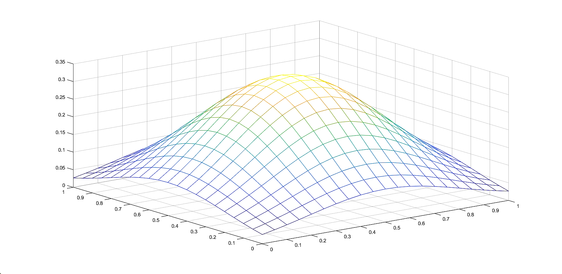
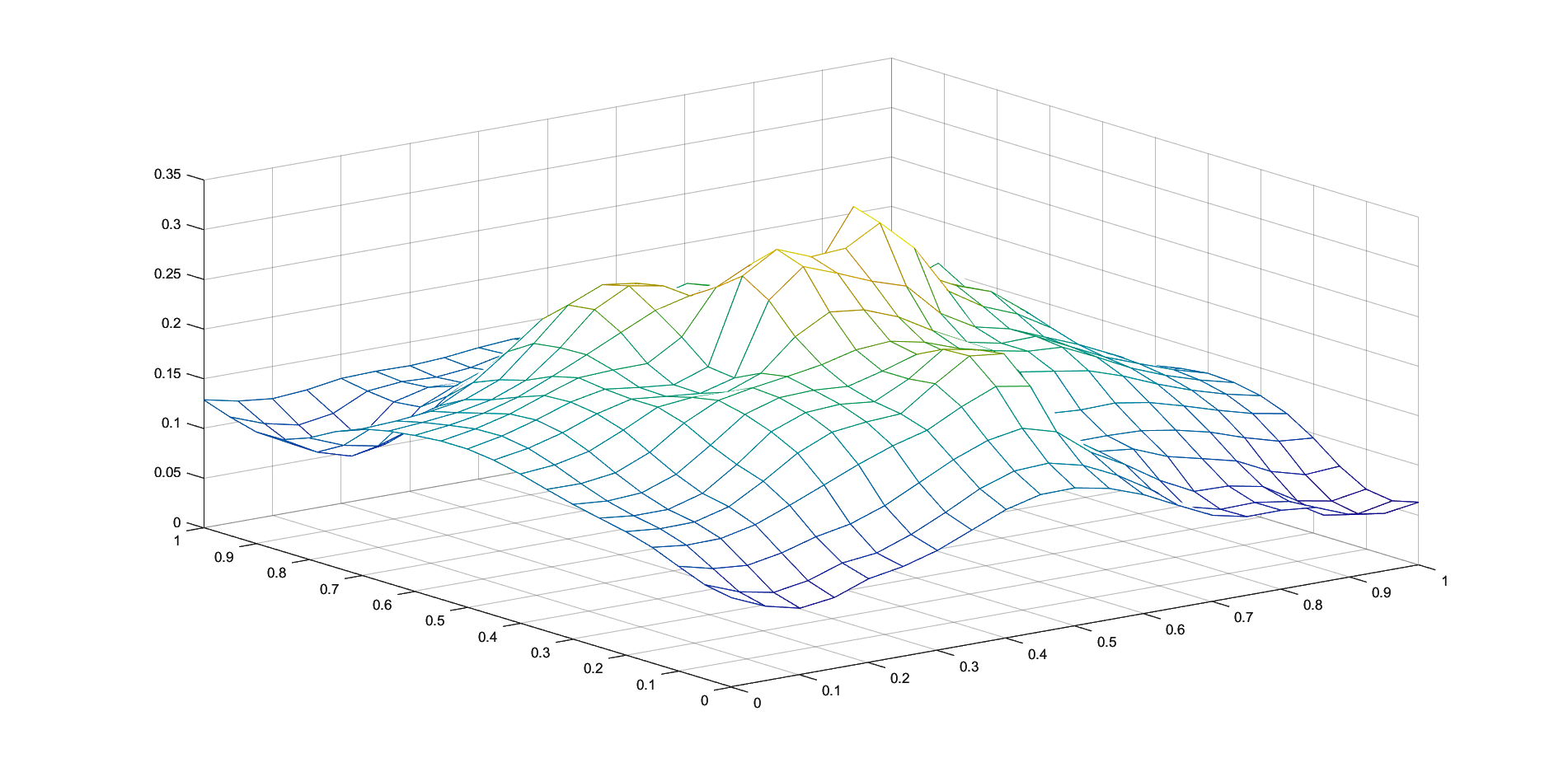
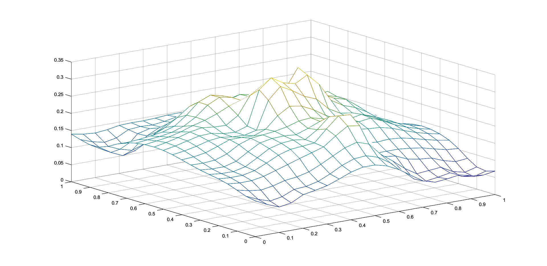
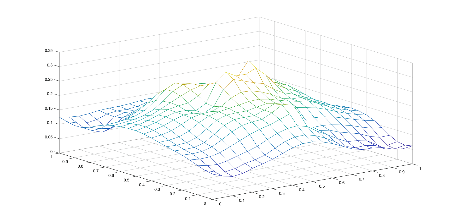
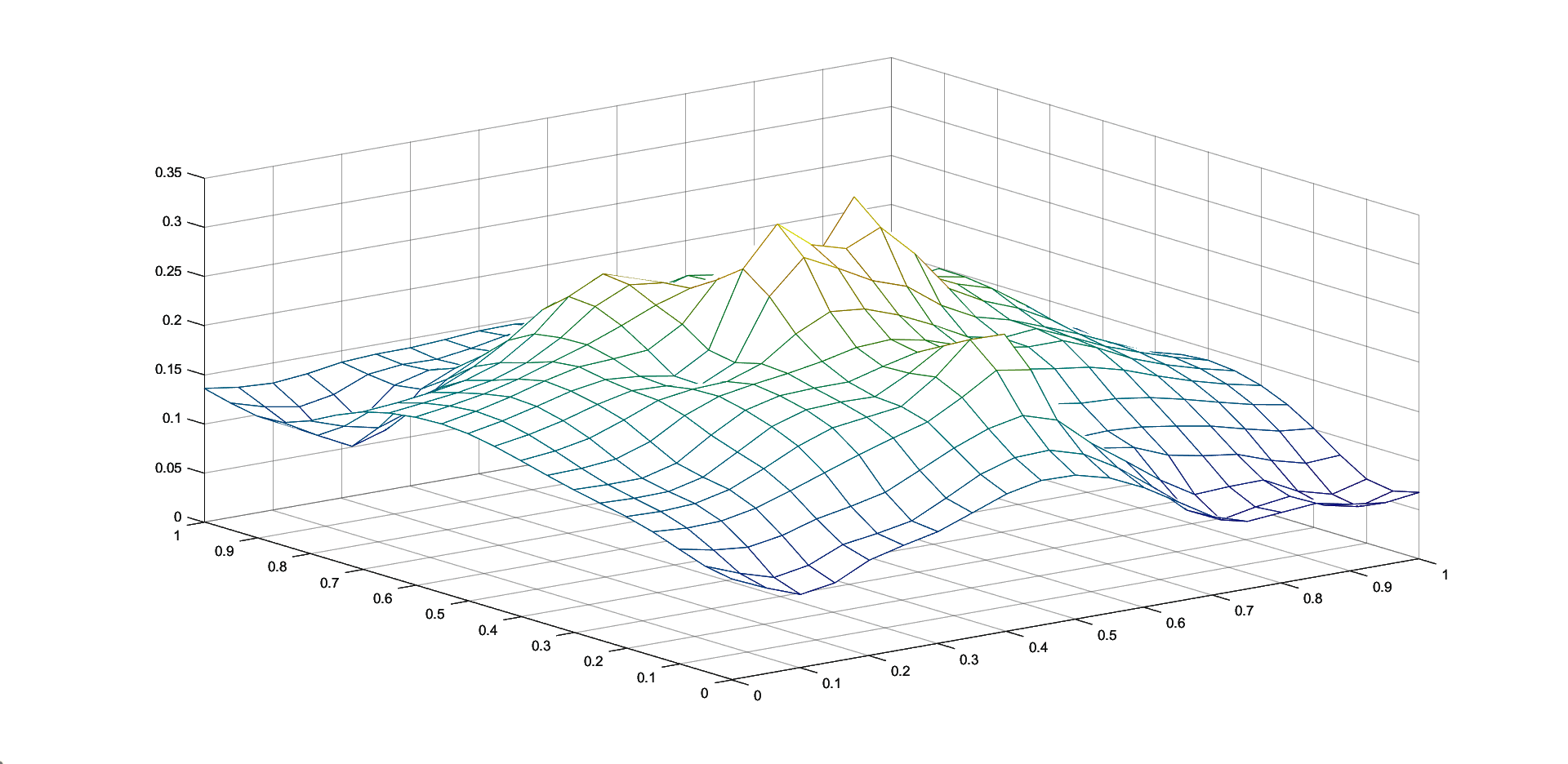
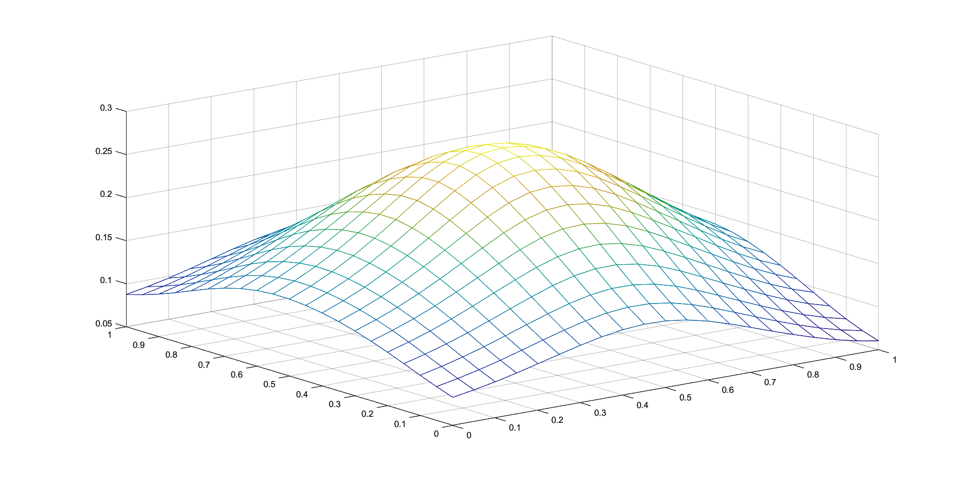
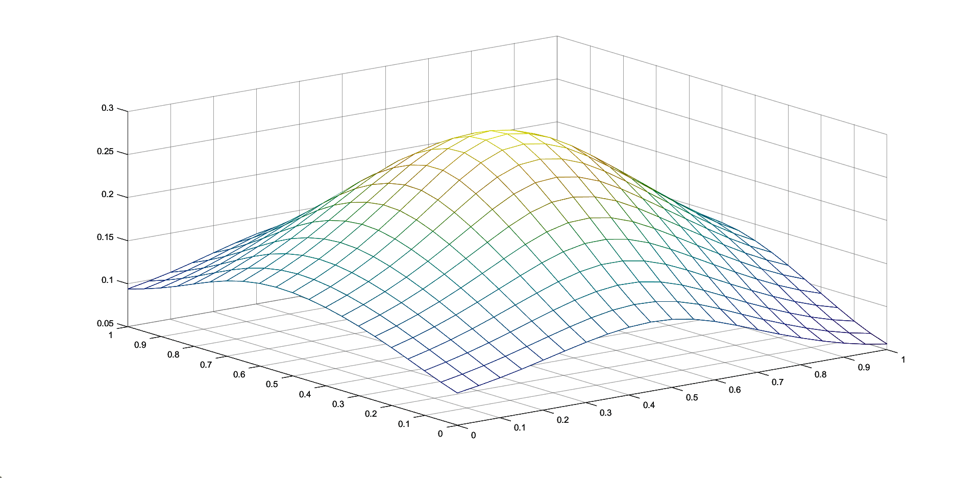
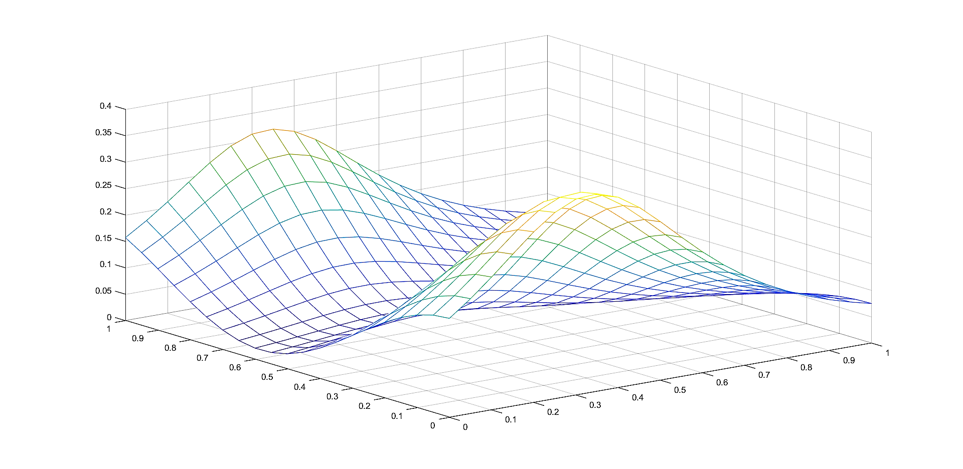
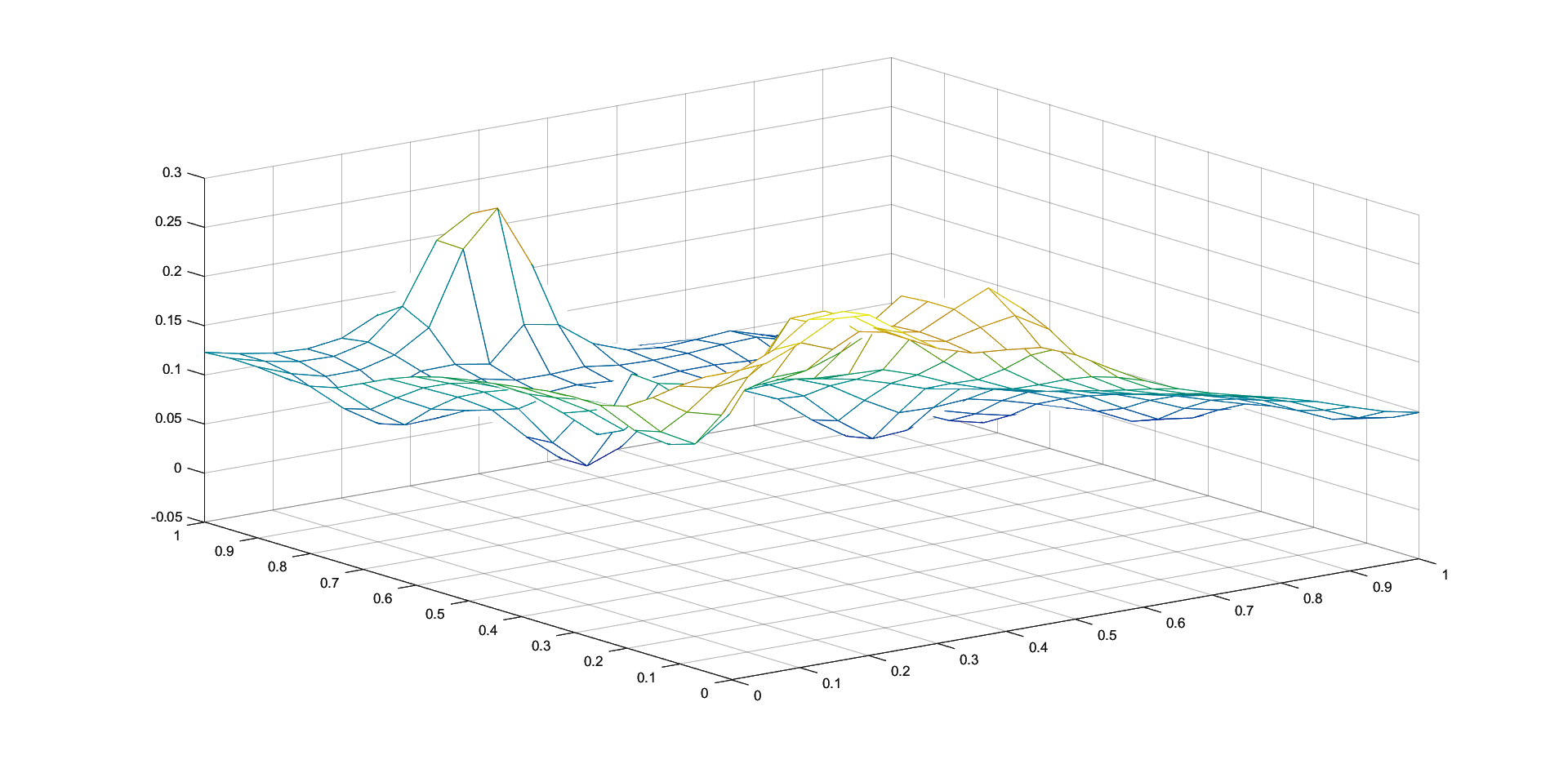
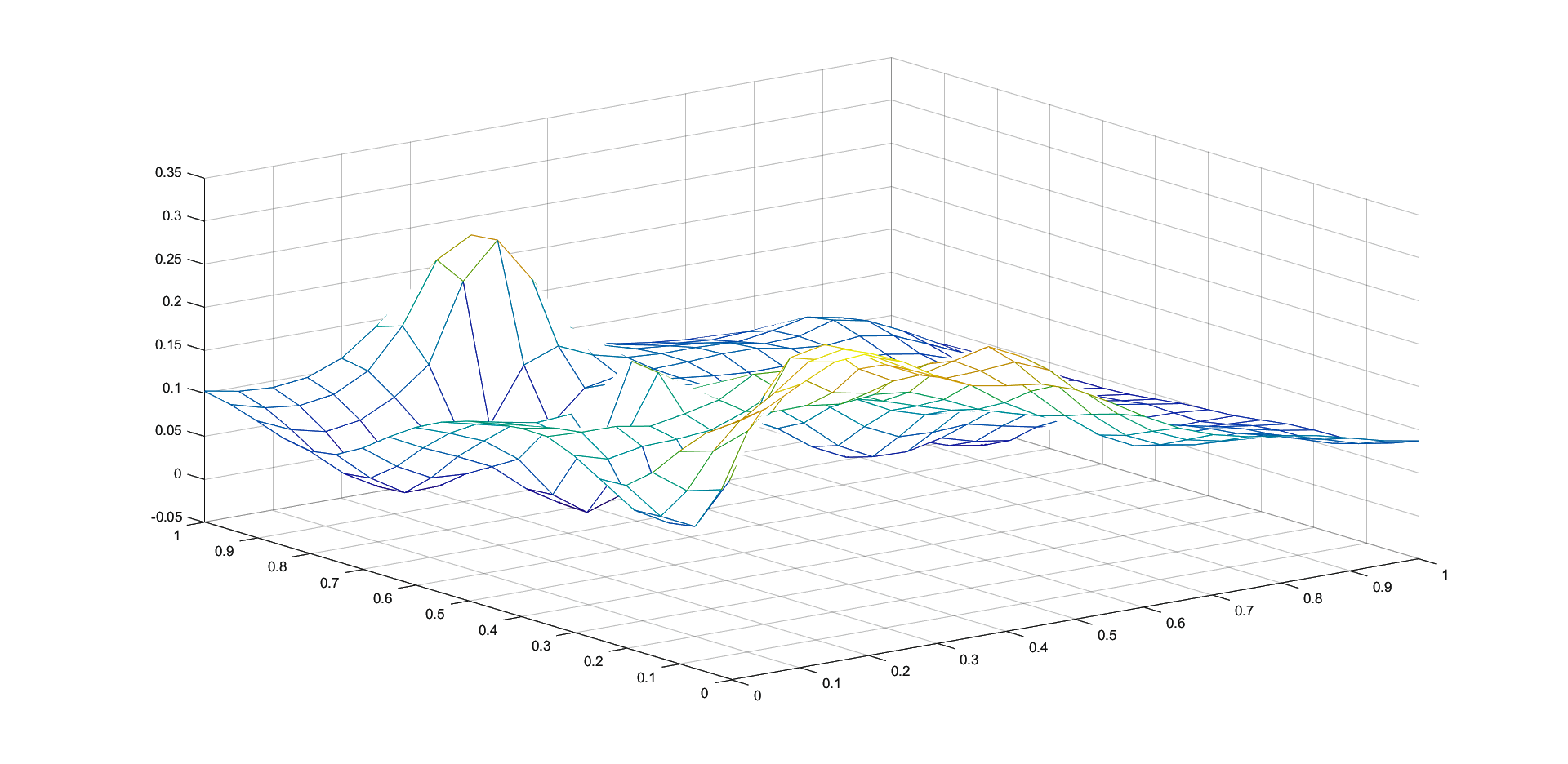
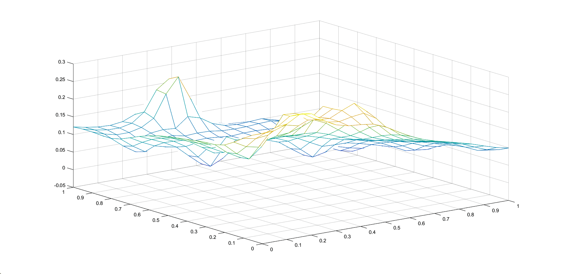
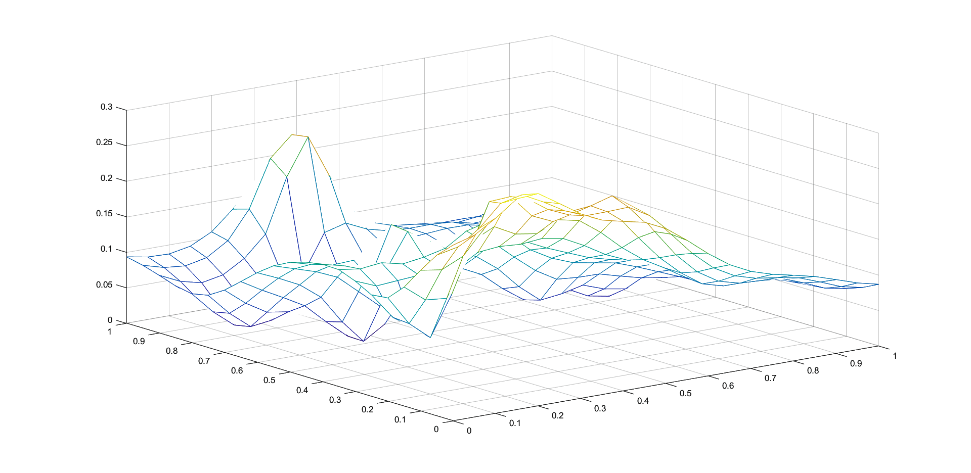
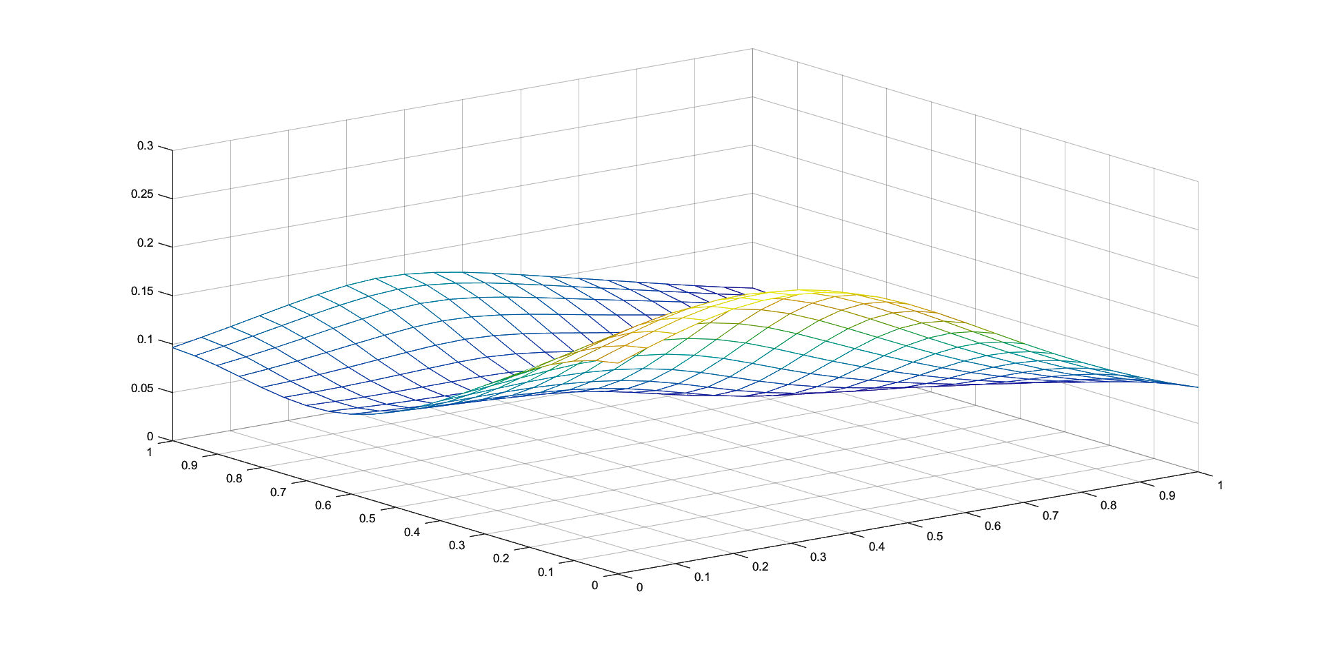
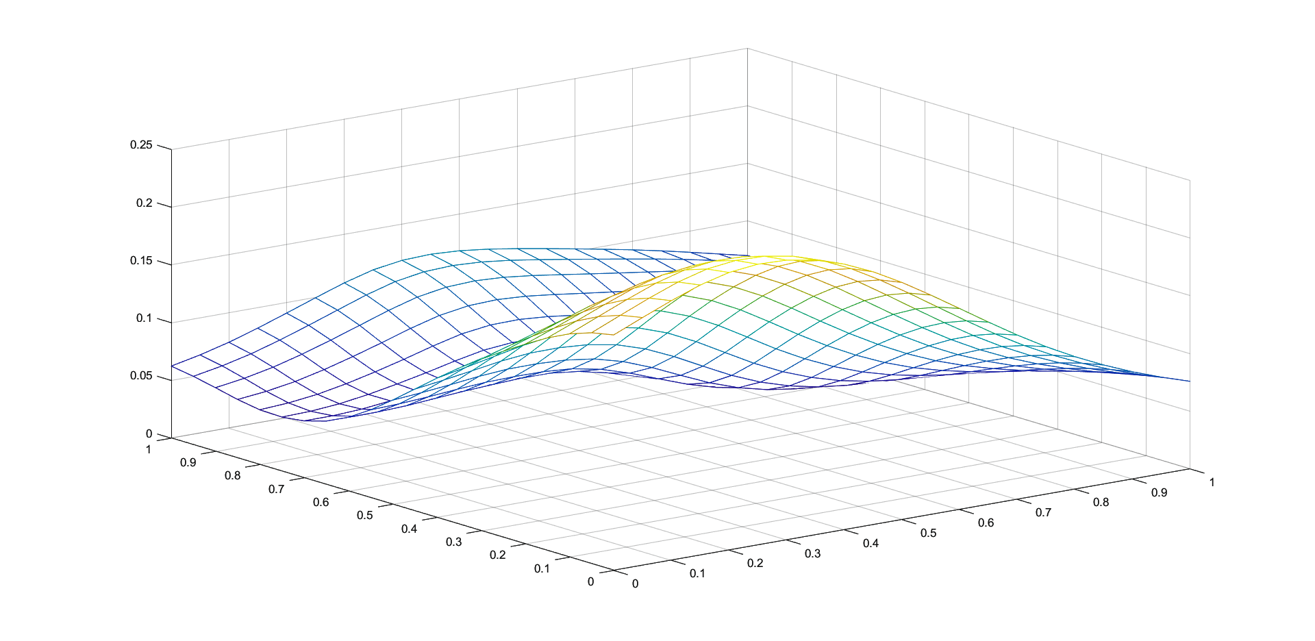
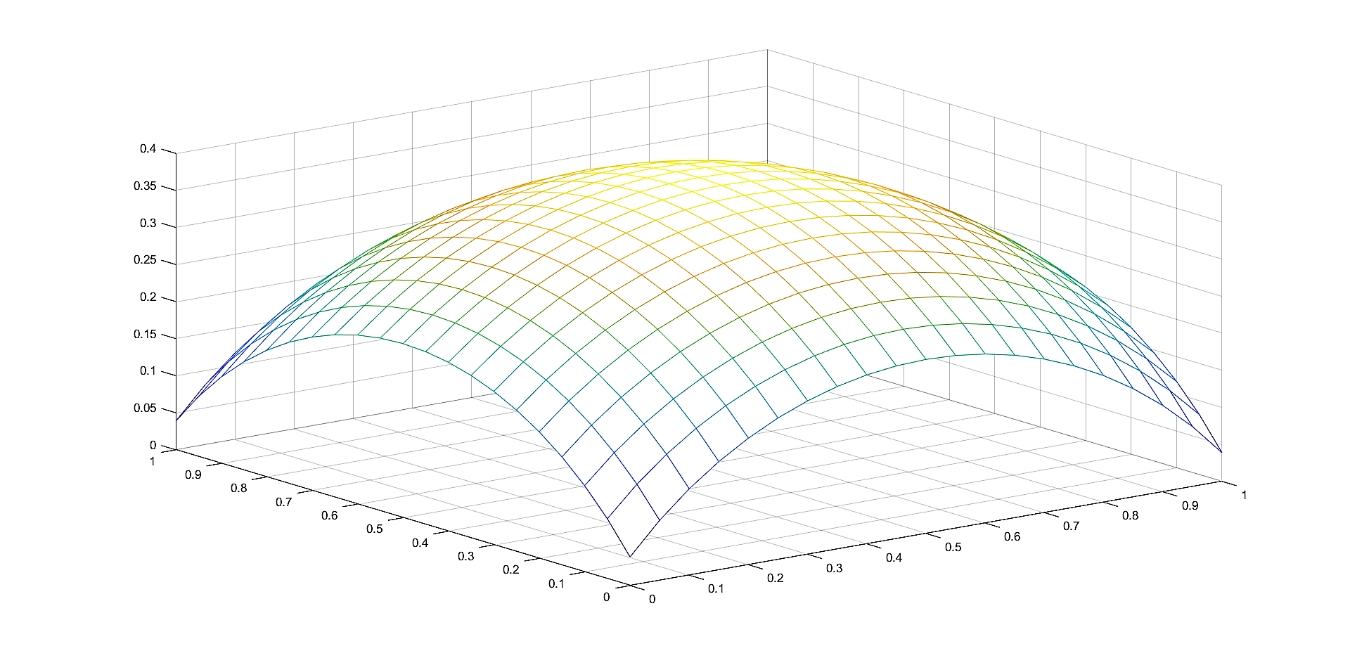
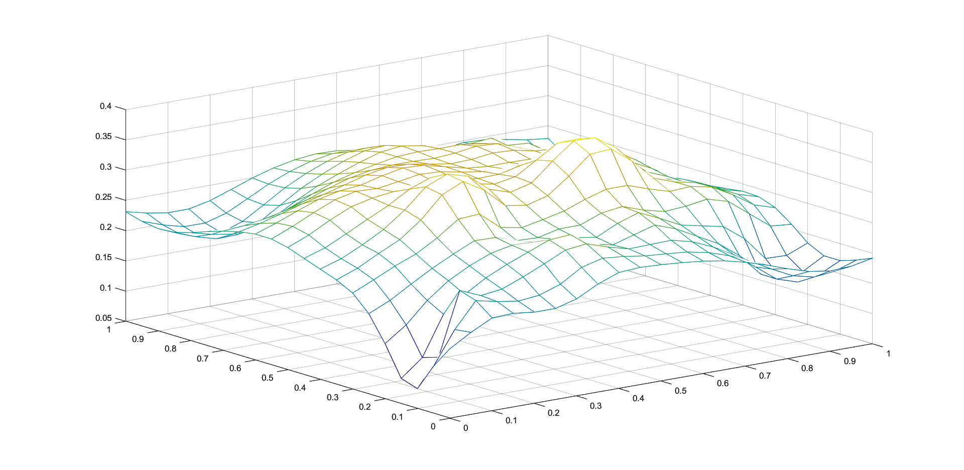
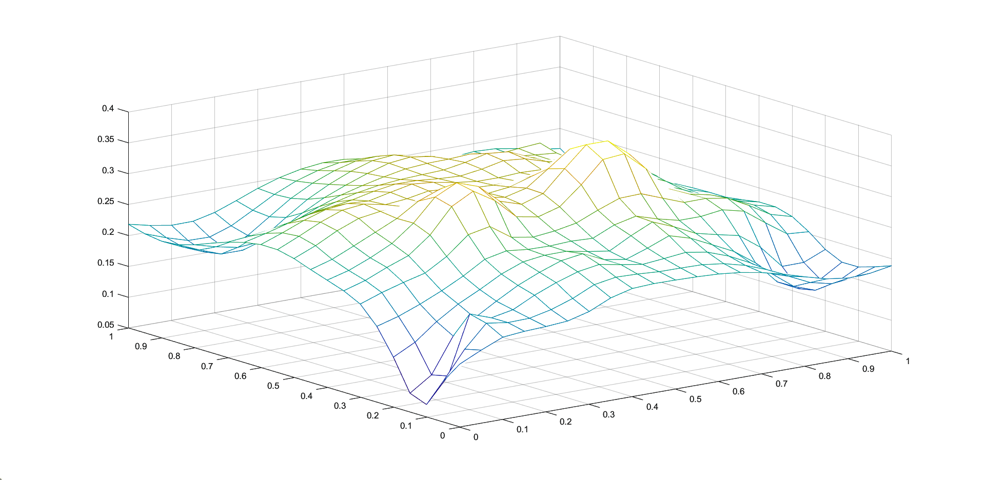
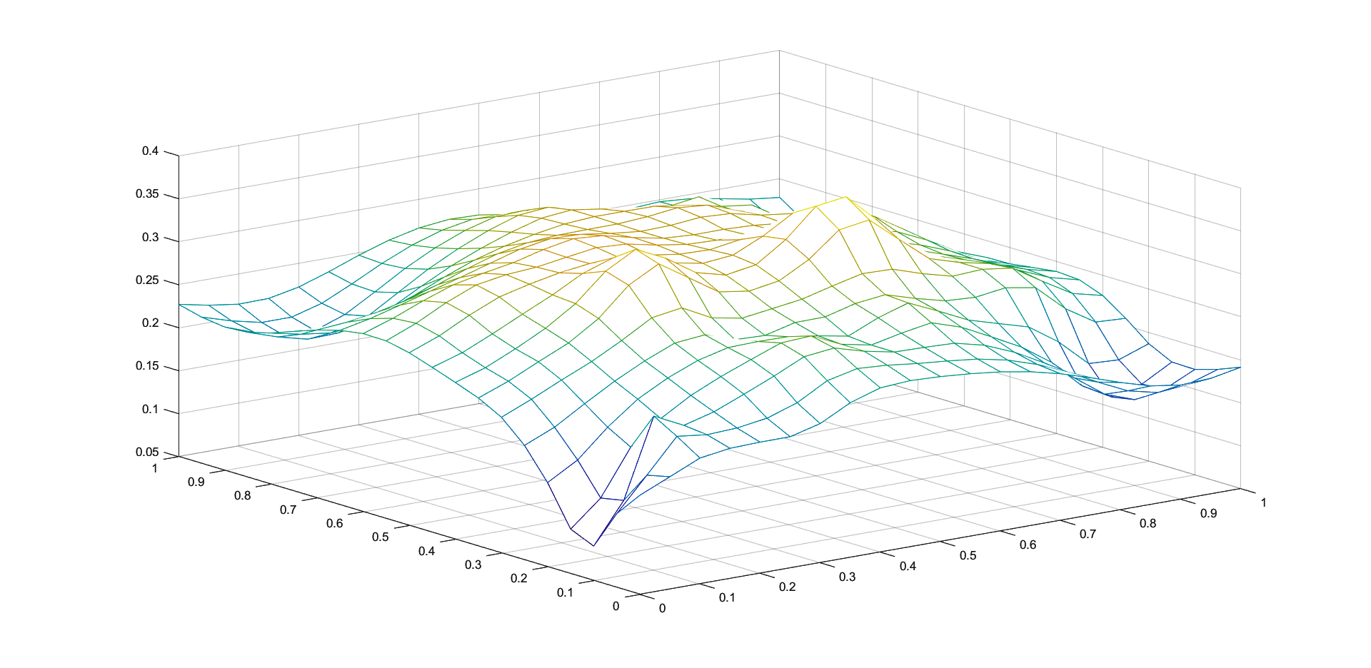
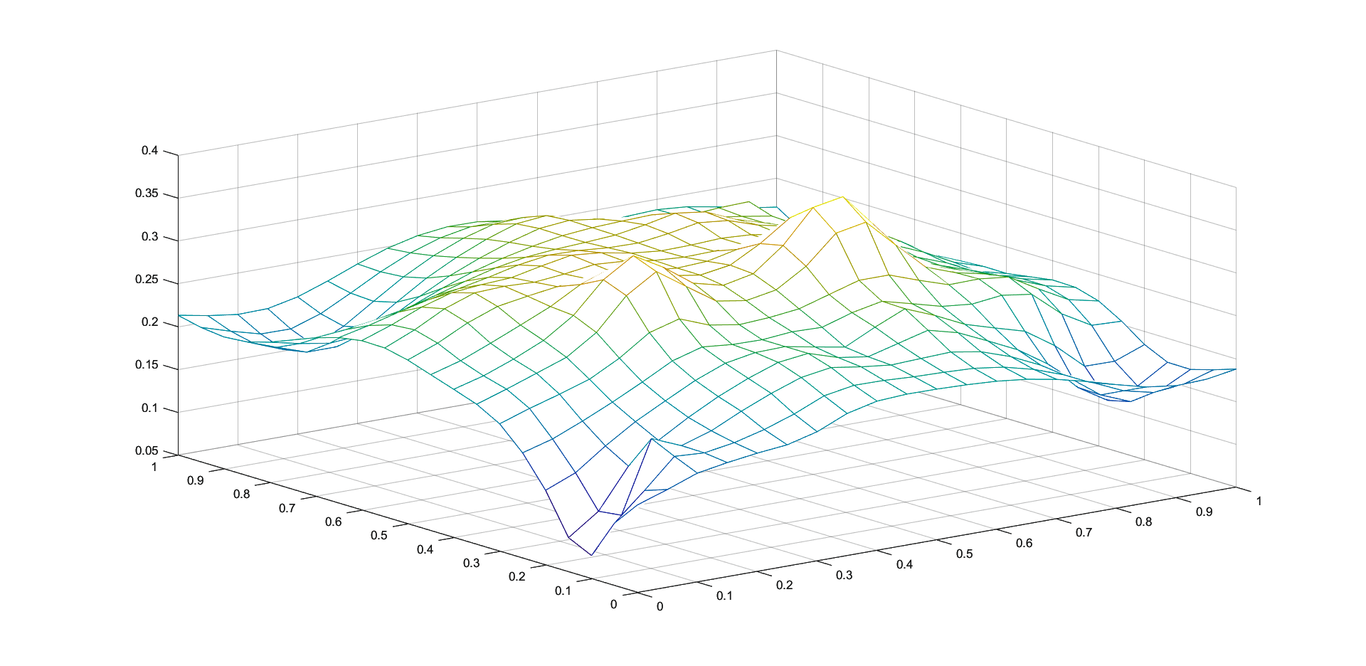
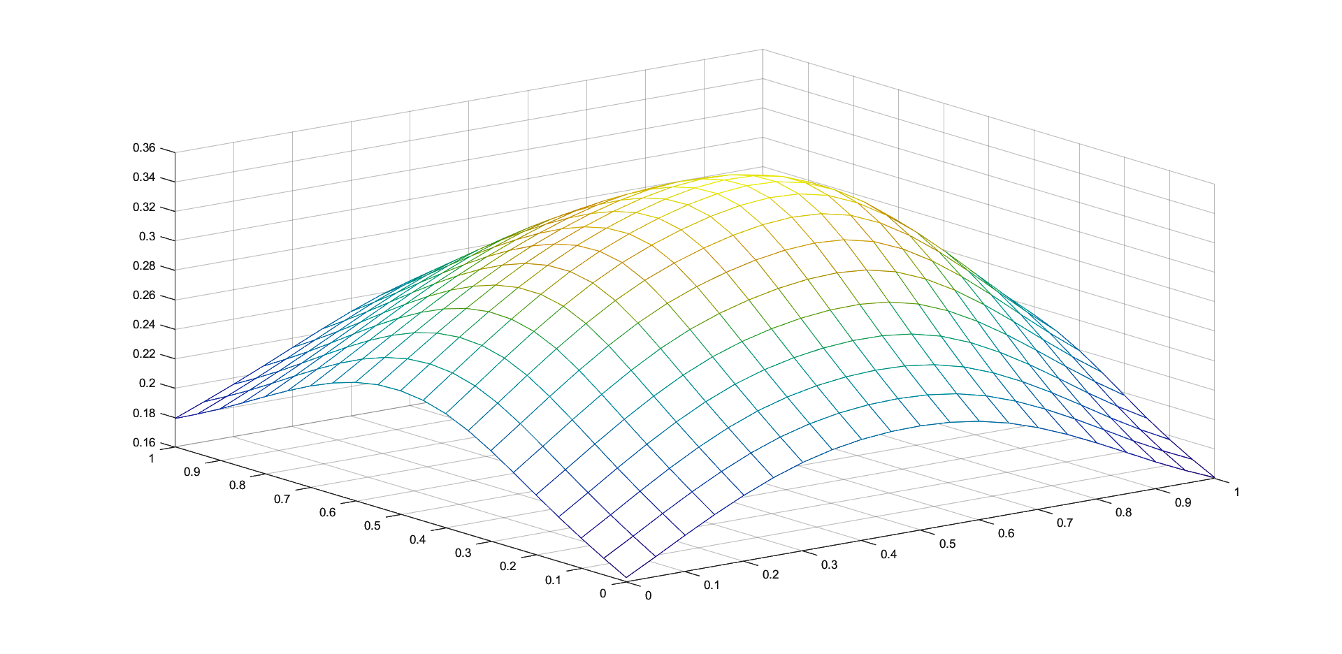
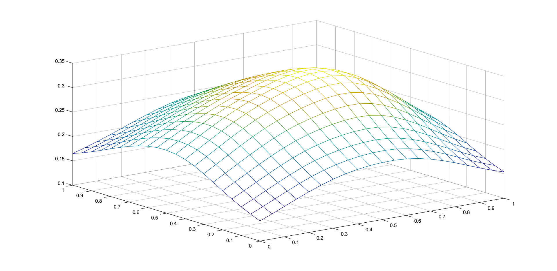
In Figures 1 - 4 we plot the graphs of and of the corresponding Shepard operators , and , combined with the inverse quadratic () and the inverse multiquadric () radial basis functions. We consider the sets of the representative knot points.
We remark that and have better approximation properties than the classical Shepard operator , the results for depending on the values of . Also, we notice better approximation errors for the lower number of knots obtained using the Algorithm 2.4.
| Classical | Modified | Iterative | ||||||
|---|---|---|---|---|---|---|---|---|
| k=25 | N=100 | k=25 | N=100 | (input) | k=25 | N=100 | ||
| – | 0.0864 | 0.0855 | 0.0725 | 0.0644 | 0.0967 | 0.1158 | ||
| 0.0757 | 0.1159 | |||||||
| 0.0528 | 0.1105 | |||||||
| 5.5 | 0.1023 | 0.5564 | 0.0994 | 0.5543 | 0.1061 | 0.2866 | ||
| 0.0847 | 0.2644 | |||||||
| 0.0627 | 0.2396 | |||||||
| 10 | 0.1313 | 0.1876 | 0.1293 | 0.1681 | 0.1026 | 0.1488 | ||
| 0.0772 | 0.1251 | |||||||
| 0.0579 | 0.1123 | |||||||
| 9 | 0.1098 | 0.2402 | 0.1063 | 0.2219 | 0.1002 | 0.2155 | ||
| 0.0866 | 0.1985 | |||||||
| 0.0686 | 0.1887 | |||||||
| 10 | 0.1129 | 0.2292 | 0.1096 | 0.2094 | 0.0994 | 0.1936 | ||
| 0.0854 | 0.1750 | |||||||
| 0.0673 | 0.1653 | |||||||
| Classical | Modified | Iterative | ||||||
|---|---|---|---|---|---|---|---|---|
| k=25 | N=100 | k=25 | N=100 | (input) | k=25 | N=100 | ||
| – | 0.1096 | 0.1152 | 0.0970 | 0.1033 | 0.2083 | 0.2051 | ||
| 0.1902 | 0.1828 | |||||||
| 0.1633 | 0.1567 | |||||||
| 7 | 0.1669 | 0.9372 | 0.1575 | 0.8615 | 0.2198 | 0.3754 | ||
| 0.2103 | 0.4007 | |||||||
| 0.1938 | 0.4456 | |||||||
| 10 | 0.1813 | 0.1693 | 0.1828 | 0.1697 | 0.2175 | 0.1909 | ||
| 0.2045 | 0.1797 | |||||||
| 0.1825 | 0.1626 | |||||||
| 9 | 0.1677 | 0.5409 | 0.1639 | 0.4933 | 0.2301 | 0.3125 | ||
| 0.2222 | 0.3202 | |||||||
| 0.2077 | 0.3344 | |||||||
| 10 | 0.1582 | 0.2952 | 0.1630 | 0.2659 | 0.2292 | 0.2000 | ||
| 0.2195 | 0.2020 | |||||||
| 0.2029 | 0.2028 | |||||||
| Classical | Modified | Iterative | ||||||
|---|---|---|---|---|---|---|---|---|
| k=25 | N=100 | k=25 | N=100 | (input) | k=25 | N=100 | ||
| – | 0.2011 | 0.2156 | 0.1934 | 0.1744 | 0.1837 | 0.1850 | ||
| 0.1730 | 0.1743 | |||||||
| 0.1593 | 0.1645 | |||||||
| 5 | 0.1849 | 1.3107 | 0.1806 | 1.1997 | 0.1576 | 0.2703 | ||
| 0.1488 | 0.4361 | |||||||
| 0.1390 | 0.5255 | |||||||
| 5.5 | 0.1926 | 0.9074 | 0.1898 | 0.8297 | 0.1637 | 0.1925 | ||
| 0.1533 | 0.2901 | |||||||
| 0.1456 | 0.3494 | |||||||
| 7 | 0.1584 | 0.8948 | 0.1526 | 0.8150 | 0.1401 | 0.2258 | ||
| 0.1291 | 0.3072 | |||||||
| 0.1183 | 0.3464 | |||||||
| 9 | 0.1796 | 0.3682 | 0.1779 | 0.3341 | 0.1537 | 0.1772 | ||
| 0.1417 | 0.2091 | |||||||
| 0.1344 | 0.2216 | |||||||
References
- [1] Buhmann, M. D., Radial basis functions, Acta Numerica, 9(2000), pp. 1–38.
- [2] Cătinaş, T., The combined Shepard-Abel-Goncharov univariate operator, Rev. Anal. Numér. Théor. Approx., 32(2003), pp. 11–20.
- [3] Cătinaş, T., The combined Shepard-Lidstone bivariate operator, In: de Bruin, M.G. et al. (eds.): Trends and Applications in Constructive Approximation. International Series of Numerical Mathematics, Springer Group-Birkhäuser Verlag, 151(2005), pp. 77–89.
- [4] Cătinaş, T., The bivariate Shepard operator of Bernoulli type, Calcolo, 44 (2007), no. 4, pp. 189-202.
- [5] Cătinaş, T., Malina, A., Shepard operator of least squares thin-plate spline type, Stud. Univ. Babeş-Bolyai Math., 66(2021), no. 2, pp. 257-265.
- [6] Coman, Gh., The remainder of certain Shepard type interpolation formulas, Studia UBB Math, 32 (1987), no. 4, pp. 24-32.
- [7] Coman, Gh., Hermite-type Shepard operators, Rev. Anal. Numér. Théor. Approx., 26(1997), 33–38.
- [8] Coman, Gh., Shepard operators of Birkhoff type, Calcolo, 35(1998), pp. 197–203.
- [9] Farwig, R., Rate of convergence of Shepard’s global interpolation formula, Math. Comp., 46(1986), pp. 577–590.
- [10] Franke, R., Scattered data interpolation: tests of some methods, Math. Comp., 38(1982), pp. 181–200.
- [11] Franke, R., Nielson, G., Smooth interpolation of large sets of scattered data, Int. J. Numer. Meths. Engrg., 15(1980), pp. 1691–1704.
- [12] Hardy, R. L., Multiquadric equations of topography and other irregular surfaces, J. Geophys. Res., 76(1971), pp. 1905–1915.
- [13] Hardy, R. L., Theory and applications of the multiquadric–biharmonic method: 20 years of discovery 1968–1988, Comput. Math. Appl., 19(1990), pp. 163–-208.
- [14] Lazzaro, D., Montefusco, L.B., Radial basis functions for multivariate interpolation of large scattered data sets, J. Comput. Appl. Math., 140(2002), pp. 521–536.
- [15] Masjukov, A.V., Masjukov, V.V., Multiscale modification of Shepard’s method for interpolation of multivariate scattered data, Mathematical Modelling and Analysis, Proceeding of the 10th International Conference MMA2005 & CMAM2, 2005, pp. 467–472.
- [16] McMahon, J. R., Knot selection for least squares approximation using thin plate splines, M.S. Thesis, Naval Postgraduate School, 1986.
- [17] McMahon, J. R., Franke, R., Knot selection for least squares thin plate splines, Technical Report, Naval Postgraduate School, Monterey, 1987.
- [18] Micchelli, C. A., Interpolation of scattered data: distance matrices and conditionally positive definite functions, Constr. Approx., 2(1986), pp. 11–22.
- [19] Renka, R.J., Cline, A.K., A triangle-based interpolation method. Rocky Mountain J. Math., 14(1984), pp. 223–237.
- [20] Renka, R.J., Multivariate interpolation of large sets of scattered data ACM Trans. Math. Software, 14(1988), pp. 139–148.
- [21] Shepard, D., A two dimensional interpolation function for irregularly spaced data, Proc. 23rd Nat. Conf. ACM, 1968, pp. 517–523.
- [22] Trîmbiţaş, G., Combined Shepard-least squares operators - computing them using spatial data structures, Studia UBB Math, 47(2002), pp. 119–128.
- [23] Zuppa, C., Error estimates for moving least square approximations, Bull. Braz. Math. Soc., New Series 34(2), 2003, pp. 231-249.
[1] Buhmann, M.D., Radial basis functions, Acta Numerica, 9(2000), 1-38.
[2] Catinas, T., The combined Shepard-Abel-Goncharov univariate operator, Rev. Anal. Numer. Theor. Approx., 32(2003), 11-20.
[3] Catinas, T., The combined Shepard-Lidstone bivariate operator, In: de Bruin, M.G. et al. (eds.): Trends and Applications in Constructive Approximation. International Series of Numerical Mathematics, Springer Group-Birkhauser Verlag, 151(2005), 77-89.
[4] Catinas, T., The bivariate Shepard operator of Bernoulli type, Calcolo, 44(2007), no. 4, 189-202.
[5] Catinas, T., Malina, A., Shepard operator of least squares thin-plate spline type, Stud. Univ. Babes-Bolyai Math., 66(2021), no. 2, 257-265.
[6] Coman, Gh., The remainder of certain Shepard type interpolation formulas, Stud. Univ. Babes-Bolyai Math., 32(1987), no. 4, 24-32.
[7] Coman, Gh., Hermite-type Shepard operators, Rev. Anal. Numer. Theor. Approx., 26(1997), 33-38.
[8] Coman, Gh., Shepard operators of Birkhoff type, Calcolo, 35(1998), 197-203.
[9] Farwig, R., Rate of convergence of Shepard’s global interpolation formula, Math. Comp., 46(1986), 577-590.
[10] Franke, R., Scattered data interpolation: tests of some methods, Math. Comp., 38(1982), 181-200.
[11] Franke, R., Nielson, G., Smooth interpolation of large sets of scattered data, Int. J. Numer. Meths. Engrg., 15(1980), 1691-1704.
[12] Hardy, R.L., Multiquadric equations of topography and other irregular surfaces, J. Geophys. Res., 76(1971), 1905-1915.
[13] Hardy, R.L., Theory and applications of the multiquadric biharmonic method: 20 years of discovery 1968-1988, Comput. Math. Appl., 19(1990), 163-208.
[14] Lazzaro, D., Montefusco, L.B., Radial basis functions for multivariate interpolation of large scattered data sets, J. Comput. Appl. Math., 140(2002), 521-536.
[15] Masjukov, A.V., Masjukov, V.V., Multiscale modification of Shepard’s method for interpolation of multivariate scattered data, Mathematical Modelling and Analysis, Proceeding of the 10th International Conference MMA2005 & CMAM2, 2005, 467-472.
[16] McMahon, J.R., Knot selection for least squares approximation using thin plate splines, M.S. Thesis, Naval Postgraduate School, 1986.
[17] McMahon, J.R., Franke, R., Knot selection for least squares thin plate splines, Technical Report, Naval Postgraduate School, Monterey, 1987.
[18] Micchelli, C.A., Interpolation of scattered data: distance matrices and conditionally positive definite functions, Constr. Approx., 2(1986), 11-22.
[19] Renka, R.J., Multivariate interpolation of large sets of scattered data, ACM Trans. Math. Software, 14(1988), 139-148.
[20] Renka, R.J., Cline, A.K., A triangle-based C1 interpolation method, Rocky Mountain J. Math., 14(1984), 223-237.
[21] Shepard, D., A two dimensional interpolation function for irregularly spaced data, Proc. 23rd Nat. Conf. ACM, 1968, 517-523.
[22] Trimbitas, G., Combined Shepard-least squares operators – computing them using spatial data structures, Stud. Univ. Babes-Bolyai Math., 47(2002), 119-128.
[23] Zuppa, C., Error estimates for moving least square approximations, Bull. Braz. Math. Soc., New Series, 34(2003), no. 2, 231-249.