Received 26 January 2012
Received in revised form 10 August 2012

Coupled reactive transport
Convergence analysis
Carbonation

© 2012 Elsevier B.V. All rights reserved.

We consider the following prototypical reaction-diffusion problem: a gaseous species $\tilde{A}$ penetrates a non-saturated porous medium via the air phase of its pore space and quickly dissolves in the pore water where $\tilde{A}$ reacts very fast with a species $\tilde{B}$. The species $\tilde{B}$ becomes available from the solid matrix by a dissolution mechanism. The reaction produces a species $\tilde{C}$ which precipitates to the porous matrix. The process can be summarized as

If the species $\tilde{A},\tilde{B}$, and $\tilde{C}$ are $\mathrm{CO}_{2},\mathrm{Ca}(\mathrm{OH})_{2}$, and respectively, $\mathrm{CaCO}_{3}$, then the reaction is called carbonation and is one of the most important processes limiting the service life of reinforced concrete. Due to carbonation, the pH of reinforced concrete drops below the passivation threshold of steel and this affects the strength of the concrete structure. The consequences may be dramatic. As common applications of reinforced concrete we mention buildings, bridges or dams (among many others). We refer to $[1,2]$ for a concise description of the details of the involved cement chemistry, existing isoline models for concrete carbonation, and of the parametric regimes when both the reaction rate of (1) and the Henry-type transfer of species $\tilde{A}$ from the gaseous phase to the liquid phase (and vice versa) can be assumed to be fast. For closely related settings arising in geochemistry, see e.g. [3-5].

Scenarios described by reaction (1) usually incorporate changes in the pore volume induced by a difference in the mass densities of $\tilde{B}$ and $\tilde{C}$. Such structural changes may locally clog the pores by a strong localized precipitation of $\tilde{C}$. In this sense we refer to [6-9] for the derivation, analysis and upscaling of mathematical models leading to dynamic, solution dependent change of the pore volumes due to dissolution and precipitation processes, or biofilm growth encountered at the pore scale. Note also that due to (1) some water is produced as well. Assuming (1) to be fast (in the spirit of [10, chapter II.5], e.g.), we expect the occurrence of localized production of water. If, on the other hand, the production is also strong, then a barrier of water might stop the penetration of the gaseous species $\tilde{A}[1]$. The challenge is to investigate under which circumstances (i.e. parameter ranges, boundary conditions, model for porosity, etc.) the clogging of the pores and the water barrier effect can take place.

The need of an adequate approximation of the fluid flow by mixed finite element method (MFEM) has been recognized in the water resources literature since several decades; see, e.g., [11]. The advantages of MFEM are: it is local mass conservative; it furnishes an accurate flux as an intrinsic part of the solution; the flux is continuous over element faces; it is applicable for strong heterogeneous media. However, the method is much more difficult to be implemented comparing to conforming finite elements (FE) and, on top of this, it is a saddle point problem and not a minimization problem. Mainly due to these reasons, for associated solute transport problems usually conventional methods are applied; e.g. FE [12,13], finite volume [14,15], discontinuous Galerkin [16] or method of characteristics [17]. In [18,19] a scheme based on MFEM is proposed also for multicomponent, reactive solute transport in soil. More precisely, the lowest order Raviart-Thomas elements are used. The drawback of being a saddle point problem is solved by hybridization [20]. In this work, we extend the scheme presented in $[18,19]$. The new features are: evolution of a concentration-dependent porosity due to production of water, and the transport coupled in both directions. Thus, we introduce and analyze a novel formulation of a fully coupled reactive multicomponent transport model and flow with variable porosity in a MFEM setting.

The convergence of numerical schemes based on MFEM (or MPFA) for flow in porous media was intensively studied in the past; see e.g. [21-26] and references cited therein. In all the mentioned work the flow of water/moisture was assumed to be independent of the diffusive transport. On the other hand, the convergence of the MFEM scheme for reactive transport in saturated/unsaturated media was analyzed in [19] (the low regularity of the solution of the flow problem has been there considered). In this paper, we derive error estimates for the fully coupled model under the assumption of a constant porosity.

The paper is structured as follows. In Section 2, we present the model equations for the reaction-diffusion-flow problem with concentration-dependent porosity announced above. The main results of the paper regarding the numerical approach are the subject of Section 3 (a numerical scheme for a reduced PDE system, including error estimates and convergence of the method). Finally, we solve the reduced PDE system and illustrate its behavior in the fast-reaction limit in Section 4.We conclude with discussions in Section 5.

We consider a porous medium occupying a domain $Y$ in $\mathbb{R}^{d},d=2$ or 3 and having the boundary $\partial Y$. We denote by $\Omega$ a reference elementary volume of our (homogeneous) material, and by $\Omega_{p}$ and $\Omega_{s}$ the volume occupied by the pores and the matrix volume, respectively. Then $\phi:=\frac{\left|\Omega_{p}\right|}{|\Omega|}$ is the porosity of the medium, while $\phi_{s}:=1-\phi$ is the corresponding solid fraction. Furthermore, $\phi_{w}:=\frac{\left|\Omega_{w}\right|}{\left|\Omega_{p}\right|}$ and $\phi_{g}:=\frac{\left|\Omega_{g}\right|}{\left|\Omega_{p}\right|}$ are the water and respectively the gas fraction. Clearly, $\phi_{w}+\phi_{g}=1$. Furthermore, we denote by $a,A,b,B,c$, and $C$ the (microscopic) molar concentrations of the species $\tilde{A}(g),\tilde{A}(aq),\tilde{B}(s),\tilde{B}(aq)$, $\tilde{C}(s)$, and $\tilde{C}(aq)$. Further, let $J=(0,T]$ be the time interval, with $T$ denoting a finite end time.

We refer to [10] for the mathematical modeling of reactive porous media flows. In particular, dissolution and precipitation Darcy-scale models are proposed in [27]. Such models can be derived rationally from pore scale models (as proposed e.g. in [28,8]) by upscaling techniques [6,7], allowing to include the variations in the porosity (including clogging) as the result of precipitation or dissolution. To maintain the discussion brief we let $\gamma$ denote the reaction rate associated to (1). Here we assume

where the constant $r>0$ has here a very large value. $p,q\in\mathbb{R}$ are partial orders of reaction that are equal or greater than unity. Throughout this work we take $p=q=1$. Eq. (2) is sometimes called generalized mass-action law. Large values of $r$ indicate the fast-reaction regime. As production rates by reaction we make use of

where $\sigma_{i}$ is the involved stoichiometric coefficient, while $m_{i}$ is the molecular weight of the species $i$. In this paper we consider reaction (1); therefore we have $\sigma_{i}=1$ for all species $\tilde{A},\tilde{B}$ and $\tilde{C}$. The production rates by precipitation and dissolution $f_{\text{Prec }}$ and $f_{\text{Diss }}$ are defined by means of deviations from known equilibrium configurations. In this paper we choose $f_{\text{Prec }}(E):=S_{\text{Prec }}\left(E-E_{p,eq}\right)$ and $f_{\text{Diss }}(E):=S_{\text{Diss }}\left(E_{d,eq}-E\right)$, where $E$ is the molecular concentration of a given species. Here
$S_{\text{Prec }}$ and $S_{\text{Diss }}$ are given constants, while $E_{d,eq}$ and $E_{p,eq}$ are known equilibrium profiles. By the choice above, a species $\tilde{E}$ is produced as long as the concentration $E$ is smaller as $E_{d,eq}$ and precipitates when the concentration $E$ is higher than $E_{p,eq}$ (see also [28,27,8]).

To state a MFEM scheme for the Eqs. (10)-(11), (12), (14), (16) and (18), we introduce the total mass fluxes of $A,B$ and $C$ :

In what follows we make use of common notations in functional analysis. By $\langle\cdot,\cdot\rangle$ we mean the inner product on $L^{2}(Y)$, or the duality pairing between $H_{0}^{1}(Y)$ and $H^{-1}(Y)$. Further, $\|\cdot\|$ and $\|\cdot\|_{1}$ stand for the norms in $L^{2}(Y)$ and $H^{1}(Y)$, respectively. The functions in $H(\operatorname{div};Y)$ are vector valued, having a $L^{2}$ divergence. By $c$ we mean a positive constant, not depending on the unknowns or the discretization parameters. We further use also the notation $\phi_{w,I}=\phi_{w}\left(p_{I}\right)$. Throughout this paper we make use of the following assumptions.
(A1) The conductivity function $k:[0,1]\rightarrow\mathbb{R}$ is strictly increasing, positive and Lipschitz continuous.
(A2) The initial concentrations $A_{I},B_{I}$, and $C_{I}$ are bounded and non-negative. The initial pressure $p_{I}$ is bounded.
(A3) For both continuous and discrete cases there holds $1\geq\phi\phi_{w}\geq\beta>0$, and $\phi_{w}$ is Lipschitz continuous.
(A4) $\mathbf{q},\mathbf{q}_{A},\mathbf{q}_{B},\mathbf{q}_{C}\in L^{\infty}(J\times Y)\cap L^{2}\left(J;H^{1}(Y)\right)$ and $\partial_{t}p,\partial_{t}A,\partial_{t}B,\partial_{t}C\in L^{\infty}(J\times Y)$.
(A5) The reaction rates are Lipschitz continuous.
Note that the assumptions on the initial data are physically natural. At the same time, (A1) and the Lipschitz continuity of $\phi_{w}$ is satisfied for several parametrization proposed in the literature (e.g. for the van Genuchten parametrization with $n\geq 2$, assuming that the medium does not become completely unsaturated). In the same spirit, the rates are Lipschitz (for the Langmuir isotherms) or at least locally Lipschitz, and the latter should be viewed in combination with the essential boundedness of the concentrations. Furthermore, the first part in (A3) states that the concrete is never becoming completely dry; under appropriate boundary and initial conditions, this is a direct consequence of the maximum principle satisfied by the Richards equation. Finally, the solution regularity in (A4) is natural for the non-degenerate case.

For simplicity, in this section we consider only homogeneous Dirichlet boundary conditions, but the results can be extended to more general cases. We assume that the system (10)-(11), (12), (14), (16) and (18) complemented with boundary and initial conditions has a unique weak solution, which solves the following problem.

Problem 3.1 (The Continuous Variational Problem). Find $p,A,B,C\in H^{1}\left(J;L^{2}(Y)\right)$ and $\mathbf{q},\mathbf{q}_{A},\mathbf{q}_{B},\mathbf{q}_{C}\in L^{2}(J;H(\operatorname{div};Y))$ with $\left.p\right|_{t=0}=p_{I},\left.A\right|_{t=0}=A_{I},\left.B\right|_{t=0}=B_{I},\left.C\right|_{t=0}=C_{I},\left.\phi\right|_{t=0}=\phi_{I}$ such that

for all $w\in L^{2}(Y)$ and $\mathbf{v}\in H(\operatorname{div};Y)$.

Referring strictly to the Richards equation (22)-(23), existence and uniqueness results are obtained e.g. in [34]. For the system (24)-(29), existence and uniqueness can be proven by following [19] at least for the case when the diffusive flux does not contain $\phi\phi_{w}$ and the porosity is constant. These results are not straightforwardly applicable to the entire system (22)-(30), which might degenerate; therefore a further study is necessary.

For the time discretization we let $N\in\mathbb{N}$ be strictly positive, and define the time step $\tau=T/N$, as well as $t_{n}=n\tau(n\in\{1,2,\ldots,N\}$ ). Given a function $f$ defined on the interval $J$, we write $f^{n}:=f\left(t_{n}\right)$. Furthermore, we let $\mathcal{T}_{h}$ be a regular decomposition of $Y\subset\mathbb{R}^{d}$ into closed $d$-simplices; $h$ stands for the mesh-size. Here we assume $\bar{Y}=\cup_{T\in\tau_{h}}T$, hence $Y$ is polygonal. We will use the discrete subspaces $W_{h}\subset L^{2}(Y)$ and $V_{h}\subset H(\operatorname{div};Y)$ defined as

In other words, $W_{h}$ denotes the space of piecewise constant functions, while $V_{h}$ is the lowest order Raviart-Thomas $RT_{0}$ space (see [20]). We will use the following $L^{2}$ projector (see [20]):

Applying a first order time stepping and MFEM, the fully discrete form of (22)-(30) reads as follows.

Problem 3.2 (The Discrete Variational Problem). Let $n\in\{1,\ldots,N\}$, and $p_{h}^{n-1},A_{h}^{n-1},B_{h}^{n-1},C_{h}^{n-1},\phi_{h}^{n-1}$ be given. Find $p_{h}^{n},A_{h}^{n},B_{h}^{n},C_{h}^{n},\phi_{h}^{n}\in W_{h}$ and $\mathbf{q}_{h}^{n},\mathbf{q}_{A_{h}}^{n},\mathbf{q}_{B_{h}}^{n},\mathbf{q}_{C_{h}}^{n}\in V_{h}$ such that for all $w_{h}\in W_{h}$ and $\mathbf{v}_{h}\in V_{h}$ there holds

and

where $\phi_{w}{}_{h}^{k}:=\phi_{w}\left(p_{h}^{k}\right),f_{\text{Diss }}{}_{h}^{k}=S_{\text{Diss }}\left(B_{eq}-B_{h}^{k}\right)$ and $f_{\text{Prec }}{}_{h}^{k}=S_{\text{Prec }}\left(C_{h}^{k}-C_{eq}\right),k=0,\ldots,N$.
Initially we take $\phi_{h}^{0}=P_{h}\phi_{I},p_{h}^{0}$ so that the following hold true: $\phi_{h}^{0}\phi_{w}^{0}=P_{h}\left(\phi_{I}\phi_{w,I}\right)$ and $A_{h}^{0}=\frac{P_{h}\left(\phi_{I}\phi_{w,I}A_{I}\right)}{\phi_{h}^{0}\phi_{w}^{0}},B_{h}^{0}=\frac{P_{h}\left(\phi_{I}\phi_{w,I}B_{I}\right)}{\phi_{h}^{0}\phi_{w}^{0}}$ and $C_{h}^{0}=\frac{P_{h}\left(\phi_{l}\phi_{w,I}C_{l}\right)}{\phi_{h}^{0}\phi_{h}^{0}}$. The particular form of the initial data is allowed by the lower bound on $\phi\phi_{w}$ and will be used in the proof of Theorem 3.1 below.

Note that Eq. (41) and the reaction in (33) are explicit. This suggests the following solution strategy, which has been adopted for the numerical calculations presented below. First of all, at each time we get the porosity from (41) and then solve (33)-(34), which is now decoupled from the remaining part of the system. Once a solution pair ( $p_{h}^{n},\mathbf{q}_{h}^{n}$ ) is computed, one can proceed by determining $\left(A_{h}^{n},\mathbf{q}_{A_{h}}^{n}\right),\left(B_{h}^{n},\mathbf{q}_{B_{h}}^{n}\right)$ and $\left(C_{h}^{n},\mathbf{q}_{C_{h}}^{n}\right)$ by solving (35)-(40).

The convergence of the scheme presented in Problem 3.2 can be shown for constant porosity (ie. $s=0$ ) and strictly unsaturated flow (when $\phi_{w}^{\prime}>0$ ) or fully saturated flow (when $\phi_{w}=\phi_{w,\text{ max }}$ everywhere). In the next we will give convergence results for these two cases. We also briefly outline the proof for the former (which is by far much more interesting as the fully saturated case). The proof is based on techniques from [35,19].

Theorem 3.1 (Strictly Unsaturated Flow). Let $s=0$ and $p,A,B,C\in H^{1}\left(J;L^{2}(Y)\right)$ and $\mathbf{q},\mathbf{q}_{A},\mathbf{q}_{B},\mathbf{q}_{C}\in L^{2}(J;H(\operatorname{div};Y))$ and $p_{h}^{n},A_{h}^{n},B_{h}^{n},C_{h}^{n}\in W_{h},\mathbf{q}_{h}^{n},\mathbf{q}_{A_{h}}^{n},\mathbf{q}_{B_{h}}^{n},\mathbf{q}_{C_{h}}^{n}\in V_{h}$ solve Problems 3.1 and 3.2, respectively. Assuming (A1)-(A5), there holds

Proof. Using results from [26] (inspired by techniques from [35]), for strictly unsaturated flow one gets

The next step is to prove a similar result for the remaining unknowns. We proceed as in [19], the main difficulty being the appearance of $\phi_{w}$ in the terms providing the $L^{2}$-estimates of the flux variables in Eqs. (25), (27) and (29) and their discrete counterparts (36), (38) and (40). We use the elementary lemma.

Lemma 3.1. For any vectors $\mathbf{a}_{k}\in\mathbb{R}^{d}$ and scalars $b_{k}\in\mathbb{R},(k\in\{1,\ldots,N\},d\geq 1)$ we have

The above lemma is an extension of the well known result for the case $b_{k}=1$, for all $k\in\{1,\ldots,N\}$. By following [19], using the lemma above and the assumed regularity for the solution one has

By (43)-(45) and the discrete Gronwall lemma we then get the result (42).
Theorem 3.2 (Fully Saturated Flow). In the strictly saturated flow regime, the result (42) becomes

We solve Eqs. (33)-(41) on $Y:=[0,1]\times[0,1]$. The initial pressure is given by $p=0.001(y-2)$. The boundary condition for the water flow are zero flux on the left and right boundaries, and $p=-0.001$ resp. $p=-0.002$ on the upper and lower boundaries (so a flux is pointing downwards). For $A,B$ and $C$ we consider homogeneous Neumann boundary conditions. For simplicity, we do not take any gravitation effects into account. As mentioned in Section 2.2, we choose the parametrization of van Genuchten-Mualem as given in (6)-(7). The following model parameters are chosen:

$\rho=1,K_{S}=2.0,\phi_{w,\max}=0.5,\alpha=0.152,n=4.0S_{\text{Diss }}=0.0067,B_{\text{eq }}=0.0075,S_{\text{Prec }}=0,C_{eq}=0,D_{A}=1.0$, $D_{B}=0.0864$ and $D_{C}=0.000864$. Further, we have $m_{A}=44,m_{B}=74,m_{C}=100.87$ and the regularization parameters $\delta=0.001,Z_{\phi}=0.01$. Initially we take $A(\mathbf{x},0)=3*10^{-3}$ on $Y_{A}^{I},A(\mathbf{x},0)=0$ on $Y\backslash Y_{A}^{I},B(\mathbf{x},0)=0.0075$ on $\Omega_{B}^{I},B(\mathbf{x},0)=0$ on $Y\backslash Y_{B}^{I}$, and $C(\mathbf{x},0)=rA(\mathbf{x},0)B(\mathbf{x},0)$. For the porosity we take $\phi_{I}=0.5$. The model is considered dimensionless; the reference values leading to the model are inspired from cement chemistry and are expressed in grams, centimeters and years, so the results should be interpreted accordingly.

For the initial domains $\Omega_{A}^{I}$ and $\Omega_{B}^{I}$ we consider three scenarios
(V1) $\left\{\begin{array}[]{l}Y_{A}^{I}=\{(x,y)\in Y\mid y\geq 0.5\}\\ Y_{B}^{I}=\{(x,y)\in Y\mid y\leq 0.53\}\end{array}\right.$
(V2) $\left\{\begin{array}[]{l}Y_{A}^{I}=\{(x,y)\in Y\mid(y\geq 0.5+0.4*x)\vee(y\geq 0.9-0.4*x)\}\\ Y_{B}^{I}=Y\backslash Y_{A}^{I}\end{array}\right.$
(V3) $\left\{\begin{array}[]{l}Y_{A}^{I}=\{(x,y)\in Y\mid(y\geq 0.5-0.4*x)\wedge(y\geq 0.1+0.4*x)\}\\ Y_{B}^{I}=Y\backslash Y_{A}^{I}.\end{array}\right.$

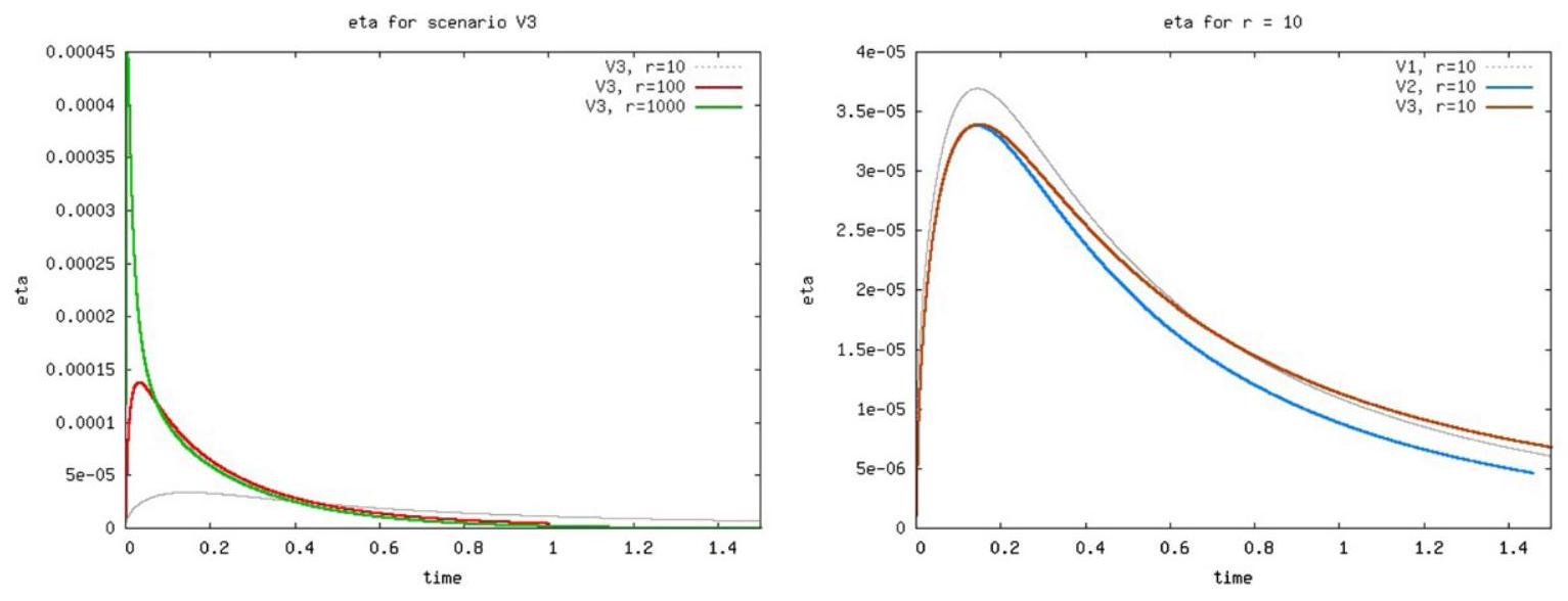
Furthermore, $A,B$ and $C$ are assumed to satisfy homogeneous Neumann boundary conditions across all sides of the square $Y$. For the degradation rate $r$, we take successively the values: 10,100 and 1000 . We compute numerically the indicator

representing the mass of $C$ produced at time $t$ by the reaction between $A$ and $B$. Further, we calculate the mass flux of the species $i,i=A,B$ or $C$ over the lower boundary $\Gamma_{S}$ (the outflow boundary, given here by $x=0$ )

The numerical scheme (33)-(41) is implemented in the software package $UG$ [36]. The computations are done with a time step $\tau=0.01$, on a regular triangular mesh with a diameter $h=0.02$ ( 5600 elements). For details of the implementation of the MFEM scheme for multicomponent, reactive transport in saturated/unsaturated media we refer to [18].

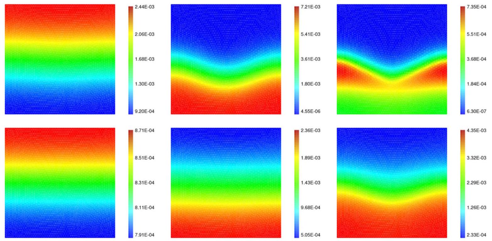
Figs. 1 and 3 illustrate the typical behavior of the concentrations $A,B$ and $C$ for one of our scenarios (V3). As expected from the model equations, we notice the consumption of concentration $A$ and subsequent production of concentration $C$. We also notice that, when choosing $r\geq 10$, we are actually simulating a reaction-diffusion-flow process in its fast-reaction regime (a high-Thiele-modulus regime). This can be observed comparing the almost "complementarity" of the colors in Figs. 1 and 3. More precisely, we observe a high production of species $C$ in those regions where $A$ is strongly depleted. These pictures indicate therefore a separation in space of free $A$-molecules from $B$-molecules that are combined in $C$ products. For low flow regimes, relying on singular-limit analyses such as [37], we expect that as $r\rightarrow\infty$ the production of $C$ will localize on free

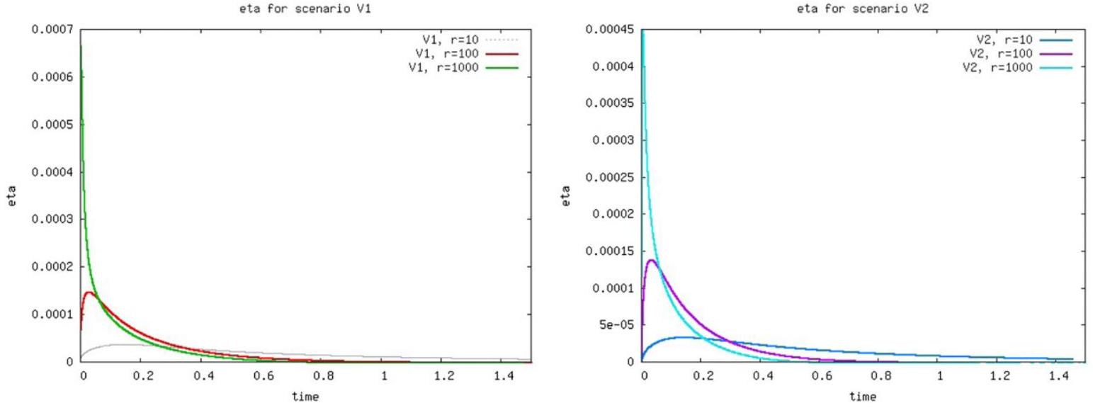
interfaces separating pockets with $A$ molecules from $B$-filled regions and $\eta\rightarrow 0$. For all three scenarios V1-V3 we observe an initial increase of $\eta$ till a maximum (the higher the peak, the higher the reaction rate $r$ ) and then a decrease to zero; see Figs. 2-5. The steepest decrease we see is for the highest rate, $r=1000$, independent of scenario. The behavior of $\eta$ is very similar for all scenarios, see Figs. 2-5, the determining factor being the reaction rate $r$. For $r=1000$ very small values of $\eta$ are reached already after short times (from 0.5 for scenario V1 to 0.8 for scenario V3), which is a strong indication of a sharp separation of species $A$ and $B$; see Fig. 5 (right).

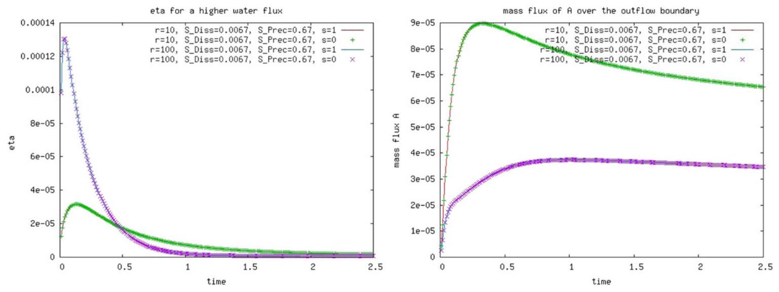
As one can see in Fig. 6 the model is very sensitive with respect to the dissolution rate $S_{\text{Diss }}$ (a higher one implies much more production of the species $B$ and also a higher maximum in $\eta$ ). In the same picture we can see but there is almost no influence of the precipitation rate $S_{\text{Prec }}$ and of a variable porosity ( $s=1$ ) on $\eta$. One reason for this is that the concentrations of $A$ and $B$ are relatively small and so also the production of $C$ and therefore the precipitation effect is neglectable. The same was confirmed also for a 1000-times higher water flux in Fig. 7 (left), where again is no difference on $\eta$ between the simulations with or without a variable porosity. We looked also at the mass fluxes of species $A-C$ over the outflow boundary, as explained in (51). The results are presented in Figs. 7 (right) and 8. There is no difference between the computations with a variable porosity and the ones without ( $s=0$ ).

To additionally validate our theoretical estimates in Section 3 we present a numerical test for an example with a known analytical solution. We solve the coupled nonlinear system of equations as given in (22)-(29) on $Y:=[0,1]\times[0,1]$. The porosity is assumed constant (thus $s=0$ in (18)) and scaled to one. The following parametrization is chosen for the

References

[1] S.A. Meier, M.A. Peter, A. Muntean, M. Böhm, Dynamics of the internal reaction layer arising during carbonation of concrete, Chem. Eng. Sci. 62(2007) 1125-1137.
[2] M.A. Peter, A. Muntean, S.A. Meier, M. Böhm, Competition of several carbonation reactions in concrete: a parametric study, Cem. Concr. Res. 38 (2008) 1385-1393.
[3] G. Auchmuty, J. Chadam, E. Merino, P. Ortoleva, E. Ripley, The structure and stability of propagating redox fronts, SIAM J. Appl. Math. 46 (1986) 588-604.
[4] P. Ortoleva, Geochemical Self-Organization, in: Oxford Monographs on Geology and Geophysics, vol. 23, Oxford University Press, NY, Oxford, 1994.
[5] S. Bauer, C. Beyer, O. Kolditz, Assesing measurement uncertainty of first-order degradation rates in heterogenous aquifers, Water Resour. Res. 42 (2006) http://dx.doi.org/10.1029/2004WRR003878.
[6] K. Kumar, T.L. van Noorden, I.S. Pop, Effective dispersion equations for reactive flows involving free boundaries at the micro-scale, Multiscale Model. Simul. 9 (2011) 29-58.
[7] T.L. van Noorden, Crystal precipitation and dissolution in a porous medium: effective equations and numerical experiments, Multiscale Model. Simul. 7 (2008) 1220-1236.
[8] T.L. van Noorden, I.S. Pop, A Stefan problem modelling dissolution and precipitation, IMA J. Appl. Math. 73 (2008) 393-411.
[9] T.L. van Noorden, I.S. Pop, A. Ebigbo, R. Helmig, An upscaled model for biofilm growth in a thin strip, Water Resour. Res. 46 (2010) W06505. http://dx.doi.org/10.1029/2009WR008217.
[10] P. Knabner, Mathematische Modelle für Transport und Sorption gelöster Stoffe in porösen Medien, Habilitationsschrift, Universität Augsburg, Germany, 1990.
[11] R. Mose, P. Siegel, P. Ackerer, G. Chavent, Application of the mixed hybrid finite element approximation in a groundwater flow model: luxury or necessity? Water Resour. Res. 30 (1994) 3001-3012.
[12] J.W. Barrett, P. Knabner, Finite element approximation of the transport of reactive solutes in porous media, part 1: error estimates for nonequilibrium adsorption processes, SIAM J. Numer. Anal. 34 (1997) 201-227.
[13] M. Bause, P. Knabner, Numerical simulation of contaminant biodegradation by higher order methods and adaptive time stepping, Comput. Vis. Sci. 7 (2004) 61-78.
[14] R. Klöfkorn, D. Kröner, M. Ohlberger, Local adaptive methods for convection dominated problems, Int. J. Numer. Methods Fluids 40(2002)79-91.
[15] M. Ohlberger, C. Rohde, Adaptive finite volume approximations of weakly coupled convection dominated problems, IMA J. Numer. Anal. 22 (2002) 253-280.
[16] B. Riviere, M.F. Wheeler, Discontinuous Galerkin methods for flow and transport problems in porous media, Comm. Numer. Methods Engrg. 18 (2002) 63-68.
[17] J. Kačur, R. van Keer, Solution of contaminant transport with adsorption in porous media by the method of characteristics, M2AN 35 (2001) 981-1006.
[18] F.A. Radu, M. Bause, A. Prechtel, S. Attinger, A mixed hybrid finite element discretization scheme for reactive transport in porous media, in: K. Kunisch, G. Of, O. Steinbach (Eds.), Numerical Mathematics and Advanced Applications, Springer Verlag, 2008, pp. 513-520.
[19] F.A. Radu, I.S. Pop, S. Attinger, Analysis of an Euler implicit-mixed finite element scheme for reactive solute transport in porous media, Numer. Methods Partial Differential Equations 26 (2009) 320-344.
[20] F. Brezzi, M. Fortin, Mixed and Hybrid Finite Element Methods, Springer-Verlag, New York, 1991.
[21] T. Arbogast, M.F. Wheeler, N.Y. Zhang, A nonlinear mixed finite element method for a degenerate parabolic equation arising in flow in porous media, SIAM J. Numer. Anal. 33 (1996) 1669-1687.
[22] R.A. Klausen, F.A. Radu, G.T. Eigestad, Convergence of MPFA on triangulations and for Richards’ equation, Int. J. Numer. Methods Fluids 58 (2008) 1327-1351.
[23] C. Woodward, C. Dawson, Analysis of expanded mixed finite element methods for a nonlinear parabolic equation modeling flow into variably saturated porous media, SIAM J. Numer. Anal. 37 (2000) 701-724.
[24] F.A. Radu, I.S. Pop, P. Knabner, Order of convergence estimates for an Euler implicit, mixed finite element discretization of Richards’ equation, SIAM J. Numer. Anal. 42 (2004) 1452-1478.
[25] F.A. Radu, I.S. Pop, P. Knabner, Error estimates for a mixed finite element discretization of some degenerate parabolic equations, Numer. Math. 109 (2008) 285-311.
[26] F.A. Radu, W. Wang, Convergence analysis for a mixed finite element scheme for flow in strictly unsaturated porous media, Nonlinear Anal. Serie B: Real World Applications (2011) http://dx.doi.org/10.1016/j.nonrwa.2011.05.003.
[27] P. Knabner, C.J. van Duijn, S. Hengst, An analysis of crystal dissolution fronts in flows through porous media-part 1: compatible boundary conditions, Adv. Water Resour. 18 (1995) 171-185.
[28] C.J. van Duijn, I.S. Pop, Crystal dissolution and precipitation in porous media: pore scale analysis, J. Reine Angew. Math. 577 (2004) 171-211.
[29] J. Bear, Y. Bachmat, Introduction to Modelling of Transport Phenomena in Porous Media, Kluwer Academic, Dordrecht, 1991.
[30] M. van Genuchten, A closed-form equation for predicting the hydraulic conductivity of unsaturated soils, Soil Sci. Soc. Am. J. 44 (1980) .
[31] Y. Mualem, A new model for predicting hydraulic conductivity of unsaturated porous media, Water Resour. Res. 12 (1976) 513-522.
[32] W.K. Lewis, W.G. Whitman, Principles of gas absorption, Ind. Eng. Chem. Res. 16 (1924) 1215-1220.
[33] X. Chen, J. Chadam, A reaction infiltration problem, part 1-existence, uniqueness, regularity and singular limit in one space dimension, Nonlinear Anal. TMA 27 (1996) 49-463.
[34] H.W. Alt, S. Luckhaus, Quasilinear elliptic-parabolic differential equations, Math. Z. 183 (1983) 311-341.
[35] T. Arbogast, M. Obeyesekere, M.F. Wheeler, Numerical methods for the simulation of flow in root-soil systems, SIAM J. Numer. Anal. 30 (1993) 1677-1702.
[36] P. Bastian, K. Birken, K. Johanssen, S. Lang, N. Neuss, H. Rentz-Reichert, C. Wieners, UG-a flexible toolbox for solving partial differential equations, Comput. Vis. Sci. 1 (1997) 27-40.
[37] T. Seidman, Interface conditions for a singular reaction-diffusion system, DCDS B 2 (2009) 631-643.